Downloaded 14 times
![An [under]view of Monte Carlo methods, from
importance sampling to MCMC, to ABC
(& kudos to Bernoulli)
Christian P. Robert
Universit´e Paris-Dauphine, University of Warwick, & CREST, Paris
2013 WSC, Hong Kong
bayesianstatistics@gmail.com](https://image.slidesharecdn.com/wsc13-130823082117-phpapp02/85/Talk-at-2013-WSC-ISI-Conference-in-Hong-Kong-August-26-2013-1-320.jpg)
![An [under]view of Monte Carlo methods, from
importance sampling to MCMC, to ABC
(& kudos to Bernoulli)
Christian P. Robert
Universit´e Paris-Dauphine, University of Warwick, & CREST, Paris
2013 WSC, Hong Kong
bayesianstatistics@gmail.com](https://image.slidesharecdn.com/wsc13-130823082117-phpapp02/75/Talk-at-2013-WSC-ISI-Conference-in-Hong-Kong-August-26-2013-1-2048.jpg)

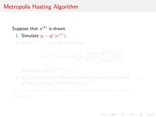
![Bernoulli as founding father of Monte Carlo methods
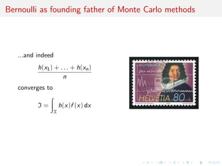
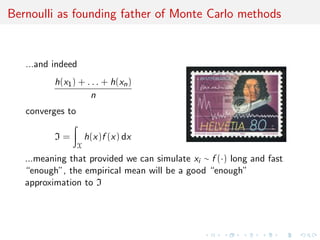
The weak law of large numbers (or Bernoulli’s [Golden] theorem)
provides the justification for Monte Carlo approximations:
if x1, . . . , xn are i.i.d. rv’s with density f ,
lim
n→∞
h(x1) + . . . + h(xn)
n
=
X
h(x)f (x) dx
Stigler’s Law of Eponimy: Cardano (1501–1576) first stated the
result](https://image.slidesharecdn.com/wsc13-130823082117-phpapp02/85/Talk-at-2013-WSC-ISI-Conference-in-Hong-Kong-August-26-2013-3-320.jpg)
![Early implementations of the LLN
While Jakob Bernoulli
himself apparently did not
engage in simulation,
Buffon (1707–1788) resorted
to a (not-yet-Monte-Carlo)
experiment in 1735 to
estimate the value of the
Saint Petersburg game
(even though he did not
perform a similar experiment
for estimating π)
[Stigler, STS, 1991; Stigler, JRSS A, 2010]](https://image.slidesharecdn.com/wsc13-130823082117-phpapp02/85/Talk-at-2013-WSC-ISI-Conference-in-Hong-Kong-August-26-2013-6-320.jpg)
![Early implementations of the LLN
While Jakob Bernoulli
himself apparently did not
engage in simulation,
De Forest (1834–1888)
found the median of a
log-Cauchy distribution,
using normal simulations
approximated to the second
digit (in 1876)
[Stigler, STS, 1991; Stigler, JRSS A, 2010]](https://image.slidesharecdn.com/wsc13-130823082117-phpapp02/85/Talk-at-2013-WSC-ISI-Conference-in-Hong-Kong-August-26-2013-7-320.jpg)
![Early implementations of the LLN
While Jakob Bernoulli
himself apparently did not
engage in simulation,
followed closely by the
ubuquitous Galton using
“normal” dice in 1890, after
developping the Quincunx,
used both for checking the
CLT and simulating from a
posterior distribution as
early as 1877
[Stigler, STS, 1991; Stigler, JRSS A, 2010]](https://image.slidesharecdn.com/wsc13-130823082117-phpapp02/85/Talk-at-2013-WSC-ISI-Conference-in-Hong-Kong-August-26-2013-8-320.jpg)
![The harmonic mean estimator
Bayesian posterior distribution defined as
π(θ|x) = π(θ)L(θ|x)/m(x)
When θi ∼ π(θ|x),
1
T
T
t=1
1
L(θt|x)
is an unbiased estimator of 1/m(x)
[Gelfand & Dey, 1994; Newton & Raftery, 1994]
Highly hazardous material: Most often leads to an infinite
variance!!!](https://image.slidesharecdn.com/wsc13-130823082117-phpapp02/85/Talk-at-2013-WSC-ISI-Conference-in-Hong-Kong-August-26-2013-13-320.jpg)
![The harmonic mean estimator
Bayesian posterior distribution defined as
π(θ|x) = π(θ)L(θ|x)/m(x)
When θi ∼ π(θ|x),
1
T
T
t=1
1
L(θt|x)
is an unbiased estimator of 1/m(x)
[Gelfand & Dey, 1994; Newton & Raftery, 1994]
Highly hazardous material: Most often leads to an infinite
variance!!!](https://image.slidesharecdn.com/wsc13-130823082117-phpapp02/85/Talk-at-2013-WSC-ISI-Conference-in-Hong-Kong-August-26-2013-14-320.jpg)
![“The Worst Monte Carlo Method Ever”
“The good news is that the Law of Large Numbers guarantees that this
estimator is consistent ie, it will very likely be very close to the correct
answer if you use a sufficiently large number of points from the posterior
distribution.
The bad news is that the number of points required for this estimator to
get close to the right answer will often be greater than the number of
atoms in the observable universe. The even worse news is that it’s easy
for people to not realize this, and to na¨ıvely accept estimates that are
nowhere close to the correct value of the marginal likelihood.”
[Radford Neal’s blog, Aug. 23, 2008]](https://image.slidesharecdn.com/wsc13-130823082117-phpapp02/85/Talk-at-2013-WSC-ISI-Conference-in-Hong-Kong-August-26-2013-15-320.jpg)
![HPD indicator as ϕ
Use the convex hull of MCMC simulations (θt)t=1,...,T
corresponding to the 10% HPD region (easily derived!) and ϕ as
indicator:
ϕ(θ) =
10
T
t∈HPD
Id(θ,θt )
[X & Wraith, 2009]](https://image.slidesharecdn.com/wsc13-130823082117-phpapp02/85/Talk-at-2013-WSC-ISI-Conference-in-Hong-Kong-August-26-2013-18-320.jpg)

![computational jam
In the 1970’s and early 1980’s, theoretical foundations of Bayesian
statistics were sound, but methodology was lagging for lack of
computing tools.
restriction to conjugate priors
limited complexity of models
small sample sizes
The field was desperately in need of a new computing paradigm!
[X & Casella, STS, 2012]](https://image.slidesharecdn.com/wsc13-130823082117-phpapp02/85/Talk-at-2013-WSC-ISI-Conference-in-Hong-Kong-August-26-2013-20-320.jpg)
![pre-Gibbs/pre-Hastings era
Early 1970’s, Hammersley, Clifford, and Besag were working on the
specification of joint distributions from conditional distributions
and on necessary and sufficient conditions for the conditional
distributions to be compatible with a joint distribution.
[Hammersley and Clifford, 1971]](https://image.slidesharecdn.com/wsc13-130823082117-phpapp02/85/Talk-at-2013-WSC-ISI-Conference-in-Hong-Kong-August-26-2013-22-320.jpg)
![pre-Gibbs/pre-Hastings era
Early 1970’s, Hammersley, Clifford, and Besag were working on the
specification of joint distributions from conditional distributions
and on necessary and sufficient conditions for the conditional
distributions to be compatible with a joint distribution.
“What is the most general form of the conditional
probability functions that define a coherent joint
function? And what will the joint look like?”
[Besag, 1972]](https://image.slidesharecdn.com/wsc13-130823082117-phpapp02/85/Talk-at-2013-WSC-ISI-Conference-in-Hong-Kong-August-26-2013-23-320.jpg)
![Hammersley-Clifford[-Besag] theorem
Theorem (Hammersley-Clifford)
Joint distribution of vector associated with a dependence graph
must be represented as product of functions over the cliques of the
graphs, i.e., of functions depending only on the components
indexed by the labels in the clique.
[Cressie, 1993; Lauritzen, 1996]](https://image.slidesharecdn.com/wsc13-130823082117-phpapp02/85/Talk-at-2013-WSC-ISI-Conference-in-Hong-Kong-August-26-2013-24-320.jpg)
![Hammersley-Clifford[-Besag] theorem
Theorem (Hammersley-Clifford)
A probability distribution P with positive and continuous density f
satisfies the pairwise Markov property with respect to an
undirected graph G if and only if it factorizes according to G, i.e.,
(F) ≡ (G)
[Cressie, 1993; Lauritzen, 1996]](https://image.slidesharecdn.com/wsc13-130823082117-phpapp02/85/Talk-at-2013-WSC-ISI-Conference-in-Hong-Kong-August-26-2013-25-320.jpg)
![Hammersley-Clifford[-Besag] theorem
Theorem (Hammersley-Clifford)
Under the positivity condition, the joint distribution g satisfies
g(y1, . . . , yp) ∝
p
j=1
g j
(y j
|y 1 , . . . , y j−1
, y j+1
, . . . , y p
)
g j
(y j
|y 1 , . . . , y j−1
, y j+1
, . . . , y p
)
for every permutation on {1, 2, . . . , p} and every y ∈ Y.
[Cressie, 1993; Lauritzen, 1996]](https://image.slidesharecdn.com/wsc13-130823082117-phpapp02/85/Talk-at-2013-WSC-ISI-Conference-in-Hong-Kong-August-26-2013-26-320.jpg)
![[Re-]Enters the Gibbs sampler
Geman and Geman (1984), building on
Metropolis et al. (1953), Hastings (1970), and
Peskun (1973), constructed a Gibbs sampler
for optimisation in a discrete image processing
problem with a Gibbs random field without
completion.
Back to Metropolis et al., 1953: the Gibbs
sampler is already in use therein and ergodicity
is proven on the collection of global maxima](https://image.slidesharecdn.com/wsc13-130823082117-phpapp02/85/Talk-at-2013-WSC-ISI-Conference-in-Hong-Kong-August-26-2013-28-320.jpg)
![[Re-]Enters the Gibbs sampler
Geman and Geman (1984), building on
Metropolis et al. (1953), Hastings (1970), and
Peskun (1973), constructed a Gibbs sampler
for optimisation in a discrete image processing
problem with a Gibbs random field without
completion.
Back to Metropolis et al., 1953: the Gibbs
sampler is already in use therein and ergodicity
is proven on the collection of global maxima](https://image.slidesharecdn.com/wsc13-130823082117-phpapp02/85/Talk-at-2013-WSC-ISI-Conference-in-Hong-Kong-August-26-2013-29-320.jpg)
![MCMC and beyond
reversible jump MCMC which impacted considerably Bayesian model
choice (Green, 1995)
adaptive MCMC algorithms (Haario & al., 1999; Roberts & Rosenthal,
2009)
exact approximations to targets (Tanner & Wong, 1987; Beaumont,
2003; Andrieu & Roberts, 2009)
comp’al stats catching up with comp’al physics: free energy sampling
(e.g., Wang-Landau), Hamilton Monte Carlo (Girolami & Calderhead,
2011)
sequential Monte Carlo (SMC) for non-sequential problems (Chopin,
2002; Neal, 2001; Del Moral et al 2006)
retrospective sampling
intractability: EP – GIMH – PMCMC – SMC2
– INLA
QMC[MC] (Owen, 2011)](https://image.slidesharecdn.com/wsc13-130823082117-phpapp02/85/Talk-at-2013-WSC-ISI-Conference-in-Hong-Kong-August-26-2013-32-320.jpg)
![Particles
Iterating/sequential importance sampling is about as old as Monte
Carlo methods themselves!
[Hammersley and Morton,1954; Rosenbluth and Rosenbluth, 1955]
Found in the molecular simulation literature of the 50’s with
self-avoiding random walks and signal processing
[Marshall, 1965; Handschin and Mayne, 1969]
Use of the term “particle” dates back to Kitagawa (1996), and Carpenter
et al. (1997) coined the term “particle filter”.](https://image.slidesharecdn.com/wsc13-130823082117-phpapp02/85/Talk-at-2013-WSC-ISI-Conference-in-Hong-Kong-August-26-2013-33-320.jpg)
![Particles
Iterating/sequential importance sampling is about as old as Monte
Carlo methods themselves!
[Hammersley and Morton,1954; Rosenbluth and Rosenbluth, 1955]
Found in the molecular simulation literature of the 50’s with
self-avoiding random walks and signal processing
[Marshall, 1965; Handschin and Mayne, 1969]
Use of the term “particle” dates back to Kitagawa (1996), and Carpenter
et al. (1997) coined the term “particle filter”.](https://image.slidesharecdn.com/wsc13-130823082117-phpapp02/85/Talk-at-2013-WSC-ISI-Conference-in-Hong-Kong-August-26-2013-34-320.jpg)
![pMC & pMCMC
Recycling of past simulations legitimate to build better
importance sampling functions as in population Monte Carlo
[Iba, 2000; Capp´e et al, 2004; Del Moral et al., 2007]
synthesis by Andrieu, Doucet, and Hollenstein (2010) using
particles to build an evolving MCMC kernel ^pθ(y1:T ) in state
space models p(x1:T )p(y1:T |x1:T )
importance sampling on discretely observed diffusions
[Beskos et al., 2006; Fearnhead et al., 2008, 2010]](https://image.slidesharecdn.com/wsc13-130823082117-phpapp02/85/Talk-at-2013-WSC-ISI-Conference-in-Hong-Kong-August-26-2013-35-320.jpg)
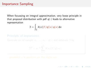
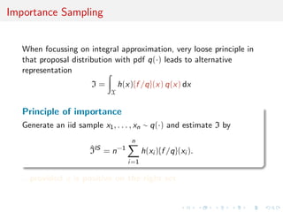
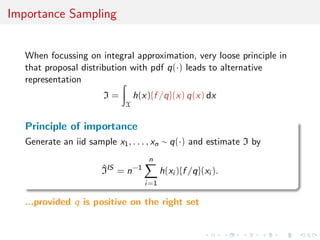
![Importance sampling perspective
1. A natural idea:
δ∗
Mn
i=1
h(zi )
p(zi )
Mn
i=1
1
p(zi )
=
Mn
i=1
π(zi )
˜π(zi )
h(zi )
Mn
i=1
π(zi )
˜π(zi )
.
2. But p not available in closed form.
3. The geometric ni is the replacement, an obvious solution that
is used in the original Metropolis–Hastings estimate since
E[ni ] = 1/p(zi ).](https://image.slidesharecdn.com/wsc13-130823082117-phpapp02/85/Talk-at-2013-WSC-ISI-Conference-in-Hong-Kong-August-26-2013-52-320.jpg)
![which Bernoulli factory?!
Not the spice warehouse of Leon Bernoulli!
Query:
Given an algorithm delivering iid B(p) rv’s, is it possible to derive
an algorithm delivering iid B(p) rv’s when f is known and p
unknown?
[von Neumann, 1951; Keane & O’Brien, 1994]
existence (e.g., impossible for f (p) = min(2p, 1))
condition: for some n,
min{f (p), 1 − f (p)} min{p, 1 − p}n
implementation (polynomial vs. exponential time)
use of sandwiching polynomials/power series](https://image.slidesharecdn.com/wsc13-130823082117-phpapp02/85/Talk-at-2013-WSC-ISI-Conference-in-Hong-Kong-August-26-2013-56-320.jpg)
![which Bernoulli factory?!
Not the spice warehouse of Leon Bernoulli!
Query:
Given an algorithm delivering iid B(p) rv’s, is it possible to derive
an algorithm delivering iid B(p) rv’s when f is known and p
unknown?
[von Neumann, 1951; Keane & O’Brien, 1994]
existence (e.g., impossible for f (p) = min(2p, 1))
condition: for some n,
min{f (p), 1 − f (p)} min{p, 1 − p}n
implementation (polynomial vs. exponential time)
use of sandwiching polynomials/power series](https://image.slidesharecdn.com/wsc13-130823082117-phpapp02/85/Talk-at-2013-WSC-ISI-Conference-in-Hong-Kong-August-26-2013-57-320.jpg)
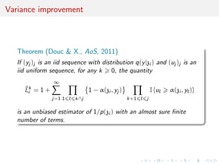
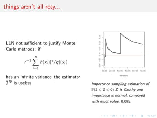
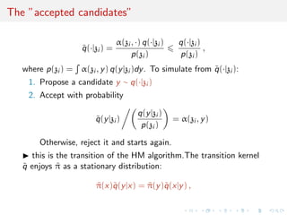
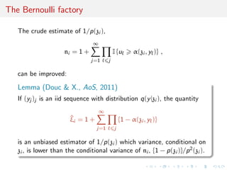
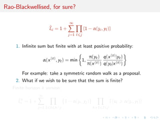
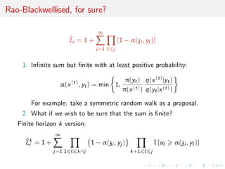
![Variance improvement
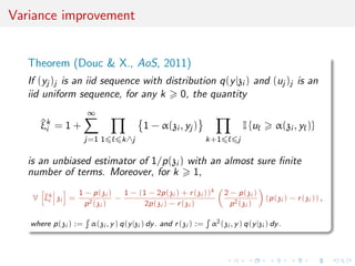
Theorem (Douc & X., AoS, 2011)
If (yj )j is an iid sequence with distribution q(y|zi ) and (uj )j is an
iid uniform sequence, for any k 0, the quantity
^ξk
i = 1 +
∞
j=1 1 k∧j
1 − α(zi , yj )
k+1 j
I {u α(zi , y )}
is an unbiased estimator of 1/p(zi ) with an almost sure finite
number of terms. Therefore, we have
V ^ξi zi V ^ξk
i zi V ^ξ0
i zi = V [ni | zi ] .](https://image.slidesharecdn.com/wsc13-130823082117-phpapp02/85/Talk-at-2013-WSC-ISI-Conference-in-Hong-Kong-August-26-2013-60-320.jpg)
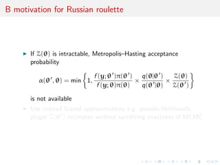
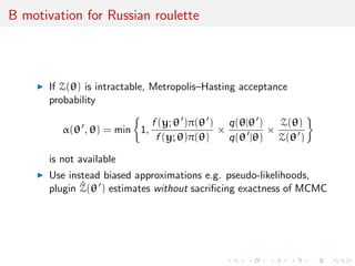
![B motivation for Russian roulette
drior π(θ), data density p(y|θ) = f (y; θ)/Z(θ) with
Z(θ) = f (x; θ)dx
intractable (e.g., Ising spin model, MRF, diffusion processes,
networks, &tc)
doubly-intractable posterior follows as
π(θ|y) = p(y|θ) × π(θ) ×
1
Z(y)
=
f (y; θ)
Z(θ)
× π(θ) ×
1
Z(y)
where Z(y) = p(y|θ)π(θ)dθ
both Z(θ) and Z(y) are intractable with massively different
consequences
[thanks to Mark Girolami for his Russian slides!]](https://image.slidesharecdn.com/wsc13-130823082117-phpapp02/85/Talk-at-2013-WSC-ISI-Conference-in-Hong-Kong-August-26-2013-61-320.jpg)
![B motivation for Russian roulette
drior π(θ), data density p(y|θ) = f (y; θ)/Z(θ) with
Z(θ) = f (x; θ)dx
intractable (e.g., Ising spin model, MRF, diffusion processes,
networks, &tc)
doubly-intractable posterior follows as
π(θ|y) = p(y|θ) × π(θ) ×
1
Z(y)
=
f (y; θ)
Z(θ)
× π(θ) ×
1
Z(y)
where Z(y) = p(y|θ)π(θ)dθ
both Z(θ) and Z(y) are intractable with massively different
consequences
[thanks to Mark Girolami for his Russian slides!]](https://image.slidesharecdn.com/wsc13-130823082117-phpapp02/85/Talk-at-2013-WSC-ISI-Conference-in-Hong-Kong-August-26-2013-62-320.jpg)
![Existing solution
Unbiased plugin estimate
Z(θ)
Z(θ )
≈
f (x; θ)
f (x; θ )
where x ∼
f (x; θ )
Z(θ )
[Møller et al, Bka, 2006; Murray et al 2006]
auxiliary variable method
removes Z(θ) Z(θ ) from the picture
require simulations from the model (e.g., via perfect sampling)](https://image.slidesharecdn.com/wsc13-130823082117-phpapp02/85/Talk-at-2013-WSC-ISI-Conference-in-Hong-Kong-August-26-2013-65-320.jpg)
![Exact approximate methods
Pseudo-Marginal construction that allows for the use of unbiased,
positive estimates of target in acceptance probability
α(θ , θ) = min 1,
^π(θ |y)
^π(θ|y)
×
q(θ|θ )
q(θ |θ)
[Beaumont, 2003; Andrieu and Roberts, 2009; Doucet et al, 2012]
Transition kernel has invariant distribution with exact target
density π(θ|y)](https://image.slidesharecdn.com/wsc13-130823082117-phpapp02/85/Talk-at-2013-WSC-ISI-Conference-in-Hong-Kong-August-26-2013-66-320.jpg)
![Exact approximate methods
Pseudo-Marginal construction that allows for the use of unbiased,
positive estimates of target in acceptance probability
α(θ , θ) = min 1,
^π(θ |y)
^π(θ|y)
×
q(θ|θ )
q(θ |θ)
[Beaumont, 2003; Andrieu and Roberts, 2009; Doucet et al, 2012]
Transition kernel has invariant distribution with exact target
density π(θ|y)](https://image.slidesharecdn.com/wsc13-130823082117-phpapp02/85/Talk-at-2013-WSC-ISI-Conference-in-Hong-Kong-August-26-2013-67-320.jpg)
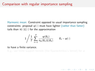
![Russian roulette
Method that requires unbiased truncation of a series
S(θ) =
∞
i=0
φi (θ)
Russian roulette employed extensively in simulation of neutron
scattering and computer graphics
Assign probabilities {qj , j 1} qj ∈ (0, 1] and generate
U(0, 1) i.i.d. r.v’s {Uj , j 1}
Find the first time k 1 such that Uk qk
Russian roulette estimate of S(θ) is
^S(θ) =
k
j=0
φj (θ)
j−1
i=1
qi ,
[Girolami, Lyne, Strathman, Simpson, & Atchad´e, arXiv:1306.4032]](https://image.slidesharecdn.com/wsc13-130823082117-phpapp02/85/Talk-at-2013-WSC-ISI-Conference-in-Hong-Kong-August-26-2013-71-320.jpg)
![Russian roulette
Method that requires unbiased truncation of a series
S(θ) =
∞
i=0
φi (θ)
Russian roulette employed extensively in simulation of neutron
scattering and computer graphics
Assign probabilities {qj , j 1} qj ∈ (0, 1] and generate
U(0, 1) i.i.d. r.v’s {Uj , j 1}
Find the first time k 1 such that Uk qk
Russian roulette estimate of S(θ) is
^S(θ) =
k
j=0
φj (θ)
j−1
i=1
qi ,
[Girolami, Lyne, Strathman, Simpson, & Atchad´e, arXiv:1306.4032]](https://image.slidesharecdn.com/wsc13-130823082117-phpapp02/85/Talk-at-2013-WSC-ISI-Conference-in-Hong-Kong-August-26-2013-72-320.jpg)
![Russian roulette
Method that requires unbiased truncation of a series
S(θ) =
∞
i=0
φi (θ)
Russian roulette employed extensively in simulation of neutron
scattering and computer graphics
Assign probabilities {qj , j 1} qj ∈ (0, 1] and generate
U(0, 1) i.i.d. r.v’s {Uj , j 1}
Find the first time k 1 such that Uk qk
Russian roulette estimate of S(θ) is
^S(θ) =
k
j=0
φj (θ)
j−1
i=1
qi ,
If limn→∞
n
j=1 qj = 0, Russian roulette terminates with
probability one
[Girolami, Lyne, Strathman, Simpson, & Atchad´e, arXiv:1306.4032]](https://image.slidesharecdn.com/wsc13-130823082117-phpapp02/85/Talk-at-2013-WSC-ISI-Conference-in-Hong-Kong-August-26-2013-73-320.jpg)
![Russian roulette
Method that requires unbiased truncation of a series
S(θ) =
∞
i=0
φi (θ)
Russian roulette employed extensively in simulation of neutron
scattering and computer graphics
Assign probabilities {qj , j 1} qj ∈ (0, 1] and generate
U(0, 1) i.i.d. r.v’s {Uj , j 1}
Find the first time k 1 such that Uk qk
Russian roulette estimate of S(θ) is
^S(θ) =
k
j=0
φj (θ)
j−1
i=1
qi ,
E{^S(θ)} = S(θ)
variance finite under certain known conditions
[Girolami, Lyne, Strathman, Simpson, & Atchad´e, arXiv:1306.4032]](https://image.slidesharecdn.com/wsc13-130823082117-phpapp02/85/Talk-at-2013-WSC-ISI-Conference-in-Hong-Kong-August-26-2013-74-320.jpg)
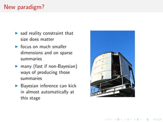
![New paradigm?
“Surprisingly, the confident prediction of the previous
generation that Bayesian methods would ultimately supplant
frequentist methods has given way to a realization that Markov
chain Monte Carlo (MCMC) may be too slow to handle
modern data sets. Size matters because large data sets stress
computer storage and processing power to the breaking point.
The most successful compromises between Bayesian and
frequentist methods now rely on penalization and
optimization.”
[Lange at al., ISR, 2013]](https://image.slidesharecdn.com/wsc13-130823082117-phpapp02/85/Talk-at-2013-WSC-ISI-Conference-in-Hong-Kong-August-26-2013-77-320.jpg)
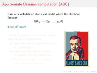
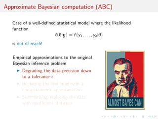
![ABC methodology
Bayesian setting: target is π(θ)f (x|θ)
When likelihood f (x|θ) not in closed form, likelihood-free rejection
technique:
Foundation
For an observation y ∼ f (y|θ), under the prior π(θ), if one keeps
jointly simulating
θ ∼ π(θ) , z ∼ f (z|θ ) ,
until the auxiliary variable z is equal to the observed value, z = y,
then the selected
θ ∼ π(θ|y)
[Rubin, 1984; Diggle & Gratton, 1984; Griffith et al., 1997]](https://image.slidesharecdn.com/wsc13-130823082117-phpapp02/85/Talk-at-2013-WSC-ISI-Conference-in-Hong-Kong-August-26-2013-83-320.jpg)
![ABC methodology
Bayesian setting: target is π(θ)f (x|θ)
When likelihood f (x|θ) not in closed form, likelihood-free rejection
technique:
Foundation
For an observation y ∼ f (y|θ), under the prior π(θ), if one keeps
jointly simulating
θ ∼ π(θ) , z ∼ f (z|θ ) ,
until the auxiliary variable z is equal to the observed value, z = y,
then the selected
θ ∼ π(θ|y)
[Rubin, 1984; Diggle & Gratton, 1984; Griffith et al., 1997]](https://image.slidesharecdn.com/wsc13-130823082117-phpapp02/85/Talk-at-2013-WSC-ISI-Conference-in-Hong-Kong-August-26-2013-84-320.jpg)
![ABC methodology
Bayesian setting: target is π(θ)f (x|θ)
When likelihood f (x|θ) not in closed form, likelihood-free rejection
technique:
Foundation
For an observation y ∼ f (y|θ), under the prior π(θ), if one keeps
jointly simulating
θ ∼ π(θ) , z ∼ f (z|θ ) ,
until the auxiliary variable z is equal to the observed value, z = y,
then the selected
θ ∼ π(θ|y)
[Rubin, 1984; Diggle & Gratton, 1984; Griffith et al., 1997]](https://image.slidesharecdn.com/wsc13-130823082117-phpapp02/85/Talk-at-2013-WSC-ISI-Conference-in-Hong-Kong-August-26-2013-85-320.jpg)
![ABC simulation advances
Simulating from the prior is often poor in efficiency
Either modify the proposal distribution on θ to increase the density
of x’s within the vicinity of y...
[Marjoram et al, 2003; Beaumont et al., 2009, Del Moral et al., 2012]
...or by viewing the problem as a conditional density estimation
and by developing techniques to allow for larger
[Beaumont et al., 2002; Blum & Fran¸cois, 2010; Biau et al., 2013]
.....or even by including in the inferential framework [ABCµ]
[Ratmann et al., 2009]](https://image.slidesharecdn.com/wsc13-130823082117-phpapp02/85/Talk-at-2013-WSC-ISI-Conference-in-Hong-Kong-August-26-2013-88-320.jpg)
![ABC simulation advances
Simulating from the prior is often poor in efficiency
Either modify the proposal distribution on θ to increase the density
of x’s within the vicinity of y...
[Marjoram et al, 2003; Beaumont et al., 2009, Del Moral et al., 2012]
...or by viewing the problem as a conditional density estimation
and by developing techniques to allow for larger
[Beaumont et al., 2002; Blum & Fran¸cois, 2010; Biau et al., 2013]
.....or even by including in the inferential framework [ABCµ]
[Ratmann et al., 2009]](https://image.slidesharecdn.com/wsc13-130823082117-phpapp02/85/Talk-at-2013-WSC-ISI-Conference-in-Hong-Kong-August-26-2013-89-320.jpg)
![ABC simulation advances
Simulating from the prior is often poor in efficiency
Either modify the proposal distribution on θ to increase the density
of x’s within the vicinity of y...
[Marjoram et al, 2003; Beaumont et al., 2009, Del Moral et al., 2012]
...or by viewing the problem as a conditional density estimation
and by developing techniques to allow for larger
[Beaumont et al., 2002; Blum & Fran¸cois, 2010; Biau et al., 2013]
.....or even by including in the inferential framework [ABCµ]
[Ratmann et al., 2009]](https://image.slidesharecdn.com/wsc13-130823082117-phpapp02/85/Talk-at-2013-WSC-ISI-Conference-in-Hong-Kong-August-26-2013-90-320.jpg)
![ABC simulation advances
Simulating from the prior is often poor in efficiency
Either modify the proposal distribution on θ to increase the density
of x’s within the vicinity of y...
[Marjoram et al, 2003; Beaumont et al., 2009, Del Moral et al., 2012]
...or by viewing the problem as a conditional density estimation
and by developing techniques to allow for larger
[Beaumont et al., 2002; Blum & Fran¸cois, 2010; Biau et al., 2013]
.....or even by including in the inferential framework [ABCµ]
[Ratmann et al., 2009]](https://image.slidesharecdn.com/wsc13-130823082117-phpapp02/85/Talk-at-2013-WSC-ISI-Conference-in-Hong-Kong-August-26-2013-91-320.jpg)
![Noisy ABC
ABC approximation error (under non-zero tolerance ) replaced
with exact simulation from a controlled approximation to the
target, convolution of true posterior with kernel function
π (θ, z|y) =
π(θ)f (z|θ)K (y − z)
π(θ)f (z|θ)K (y − z)dzdθ
,
with K kernel parameterised by bandwidth .
[Wilkinson, 2013]
Theorem
The ABC algorithm based on a randomised observation y = ˜y + ξ,
ξ ∼ K , and an acceptance probability of
K (y − z)/M
gives draws from the posterior distribution π(θ|y).](https://image.slidesharecdn.com/wsc13-130823082117-phpapp02/85/Talk-at-2013-WSC-ISI-Conference-in-Hong-Kong-August-26-2013-95-320.jpg)
![Noisy ABC
ABC approximation error (under non-zero tolerance ) replaced
with exact simulation from a controlled approximation to the
target, convolution of true posterior with kernel function
π (θ, z|y) =
π(θ)f (z|θ)K (y − z)
π(θ)f (z|θ)K (y − z)dzdθ
,
with K kernel parameterised by bandwidth .
[Wilkinson, 2013]
Theorem
The ABC algorithm based on a randomised observation y = ˜y + ξ,
ξ ∼ K , and an acceptance probability of
K (y − z)/M
gives draws from the posterior distribution π(θ|y).](https://image.slidesharecdn.com/wsc13-130823082117-phpapp02/85/Talk-at-2013-WSC-ISI-Conference-in-Hong-Kong-August-26-2013-96-320.jpg)
![Which summary?
Fundamental difficulty of the choice of the summary statistic when
there is no non-trivial sufficient statistics [except when done by the
experimenters in the field]](https://image.slidesharecdn.com/wsc13-130823082117-phpapp02/85/Talk-at-2013-WSC-ISI-Conference-in-Hong-Kong-August-26-2013-97-320.jpg)
![Which summary?
Fundamental difficulty of the choice of the summary statistic when
there is no non-trivial sufficient statistics [except when done by the
experimenters in the field]
Loss of statistical information balanced against gain in data
roughening
Approximation error and information loss remain unknown
Choice of statistics induces choice of distance function
towards standardisation
borrowing tools from data analysis (LDA) machine learning
[Estoup et al., ME, 2012]](https://image.slidesharecdn.com/wsc13-130823082117-phpapp02/85/Talk-at-2013-WSC-ISI-Conference-in-Hong-Kong-August-26-2013-98-320.jpg)
![Which summary?
Fundamental difficulty of the choice of the summary statistic when
there is no non-trivial sufficient statistics [except when done by the
experimenters in the field]
may be imposed for external/practical reasons
may gather several non-B point estimates
we can learn about efficient combination
distance can be provided by estimation techniques](https://image.slidesharecdn.com/wsc13-130823082117-phpapp02/85/Talk-at-2013-WSC-ISI-Conference-in-Hong-Kong-August-26-2013-99-320.jpg)
![Which summary for model choice?
‘This is also why focus on model discrimination typically (...)
proceeds by (...) accepting that the Bayes Factor that one obtains
is only derived from the summary statistics and may in no way
correspond to that of the full model.’
[S. Sisson, Jan. 31, 2011, xianblog]
Depending on the choice of η(·), the Bayes factor based on this
insufficient statistic,
Bη
12(y) =
π1(θ1)f η
1 (η(y)|θ1) dθ1
π2(θ2)f η
2 (η(y)|θ2) dθ2
,
is either consistent or not
[X et al., PNAS, 2012]](https://image.slidesharecdn.com/wsc13-130823082117-phpapp02/85/Talk-at-2013-WSC-ISI-Conference-in-Hong-Kong-August-26-2013-100-320.jpg)
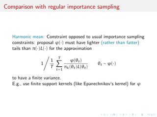
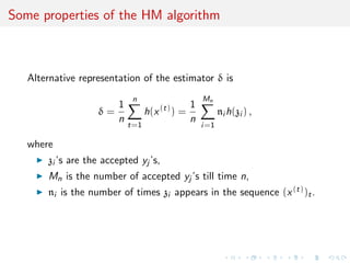
![Which summary for model choice?
Depending on the choice of η(·), the Bayes factor based on this
insufficient statistic,
Bη
12(y) =
π1(θ1)f η
1 (η(y)|θ1) dθ1
π2(θ2)f η
2 (η(y)|θ2) dθ2
,
is either consistent or not
[X et al., PNAS, 2012]
q
q
q
q
q
q
q
q
q
q
q
Gauss Laplace
0.00.10.20.30.40.50.60.7
n=100
q
q
q
q
q
q
q
q
q
q
q
q
q
q
q
q
q
q
Gauss Laplace
0.00.20.40.60.81.0
n=100](https://image.slidesharecdn.com/wsc13-130823082117-phpapp02/85/Talk-at-2013-WSC-ISI-Conference-in-Hong-Kong-August-26-2013-101-320.jpg)
![Selecting proper summaries
Consistency only depends on the range of
µi (θ) = Ei [η(y)]
under both models against the asymptotic mean µ0 of η(y)
Theorem
If Pn belongs to one of the two models and if µ0 cannot be
attained by the other one :
0 = min (inf{|µ0 − µi (θi )|; θi ∈ Θi }, i = 1, 2)
< max (inf{|µ0 − µi (θi )|; θi ∈ Θi }, i = 1, 2) ,
then the Bayes factor Bη
12 is consistent
[Marin et al., JRSS B, 2013]](https://image.slidesharecdn.com/wsc13-130823082117-phpapp02/85/Talk-at-2013-WSC-ISI-Conference-in-Hong-Kong-August-26-2013-102-320.jpg)
![Selecting proper summaries
Consistency only depends on the range of
µi (θ) = Ei [η(y)]
under both models against the asymptotic mean µ0 of η(y)
q
M1 M2
0.30.40.50.60.7
q
q
q
q
M1 M2
0.30.40.50.60.7
M1 M2
0.30.40.50.60.7
q
q
q
q
q
q
q
q
M1 M2
0.00.20.40.60.8
q
qq
q
q
q
q
q
q
q
q
qq
q
q
q
q
q
q
M1 M2
0.00.20.40.60.81.0
q
q
q
q
q
q
q
q
M1 M2
0.00.20.40.60.81.0
q
q
q
q
q
q
q
M1 M2
0.00.20.40.60.8
q
q
qq
q
q
q
q
qq
q
q
q
q
q
q
q
M1 M2
0.00.20.40.60.81.0
q
q
qq
q
qq
M1 M2
0.00.20.40.60.81.0
[Marin et al., JRSS B, 2013]](https://image.slidesharecdn.com/wsc13-130823082117-phpapp02/85/Talk-at-2013-WSC-ISI-Conference-in-Hong-Kong-August-26-2013-103-320.jpg)

The document provides an extensive exploration of Monte Carlo methods from importance sampling to Markov Chain Monte Carlo (MCMC) and Approximate Bayesian Computation (ABC), highlighting key contributions from Jakob Bernoulli and others in advancing these statistical techniques. It discusses the foundational principles of these methods alongside historical context and the evolution of computational approaches in Bayesian statistics. Additionally, it outlines various algorithms like the Gibbs and Metropolis-Hastings algorithms, emphasizing their impact and applications across different fields of study.


![Inference in generative models using the Wasserstein distance [[INI]](https://cdn.slidesharecdn.com/ss_thumbnails/inewton-170706120746-thumbnail.jpg?width=640&height=640&fit=bounds)


