Download as PDF, PPTX

![Markov Chain Monte Carlo Methods
The Metropolis-Hastings Algorithm
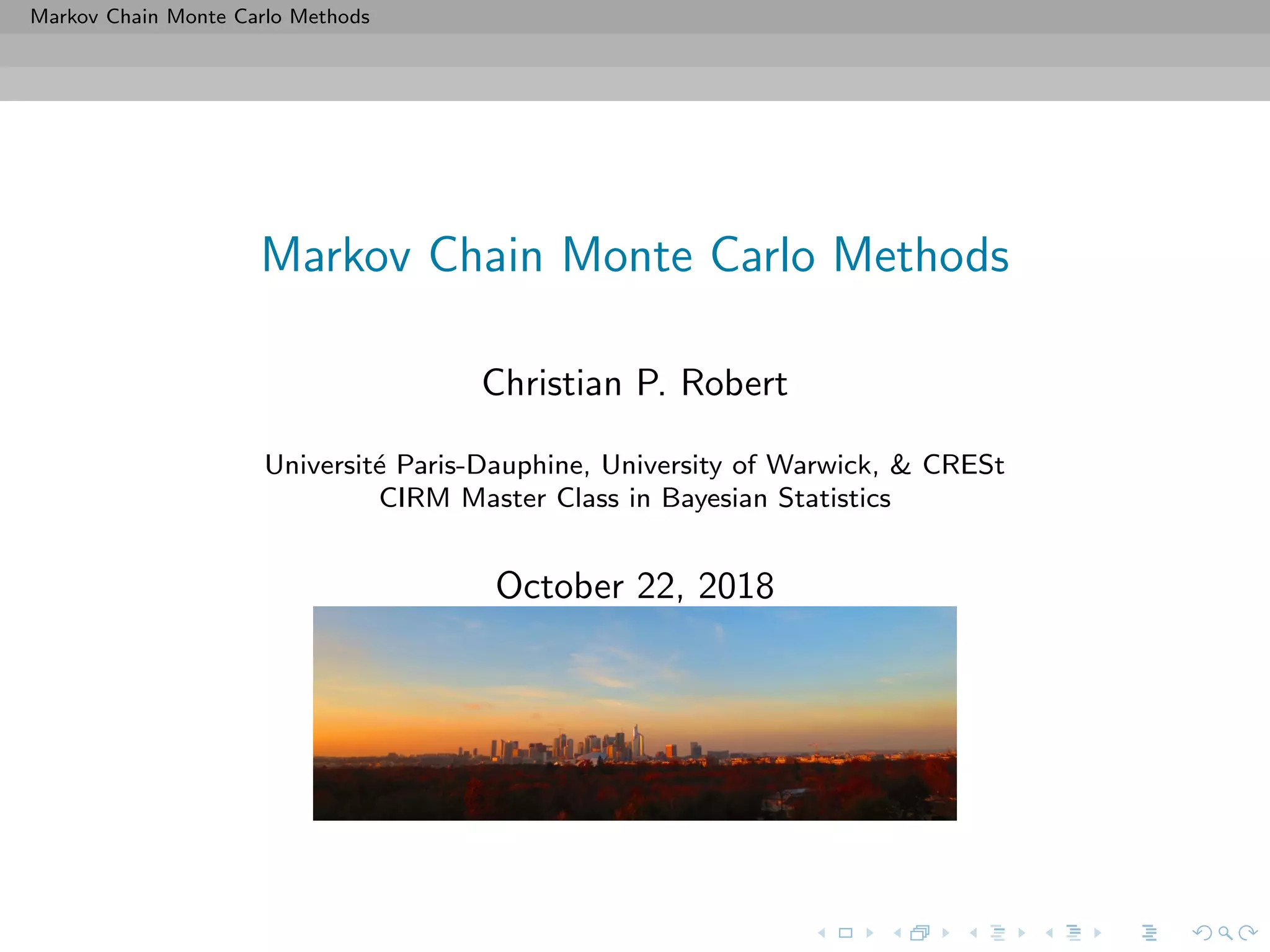
The Metropolis–Hastings algorithm
The Metropolis–Hastings algorithm
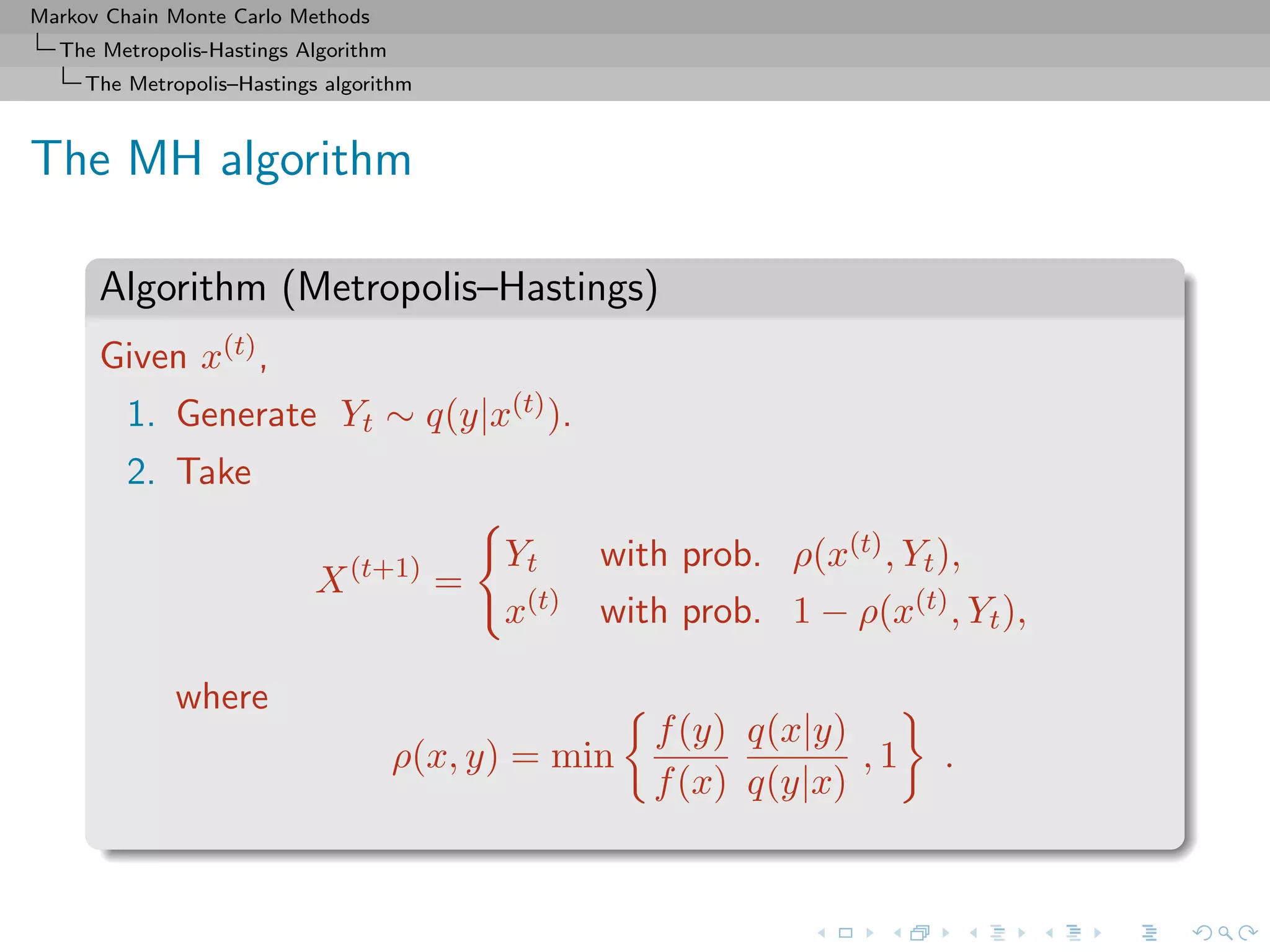
Basics
The algorithm uses the objective
(target) density
f
and a conditional density
q(y|x)
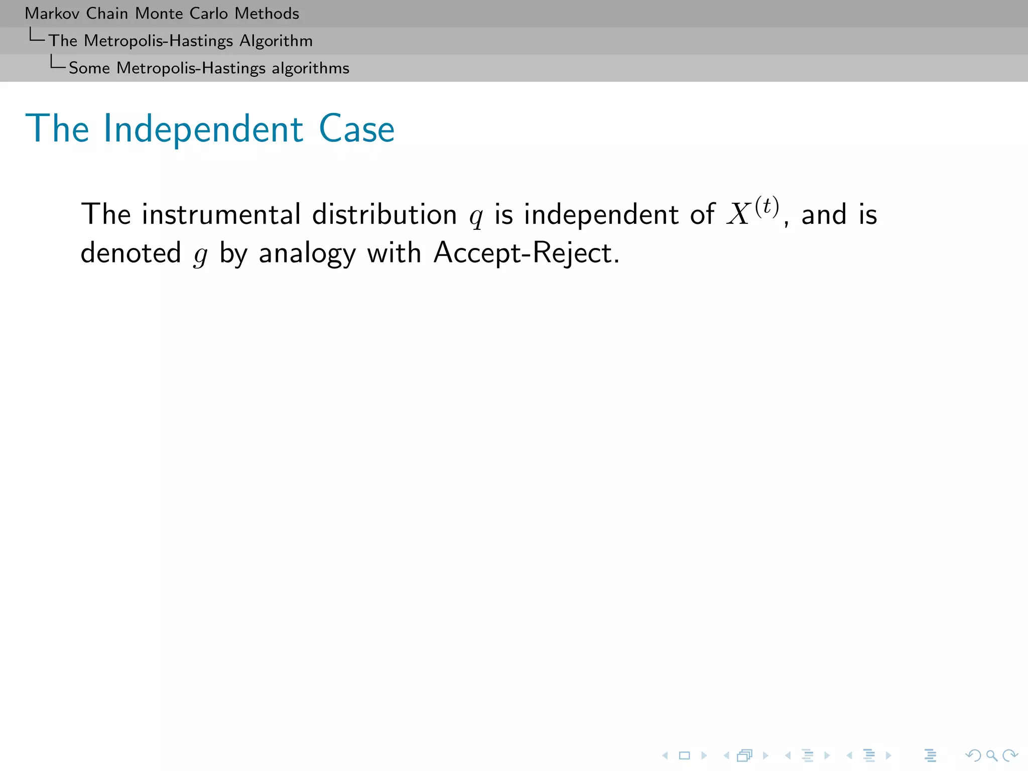
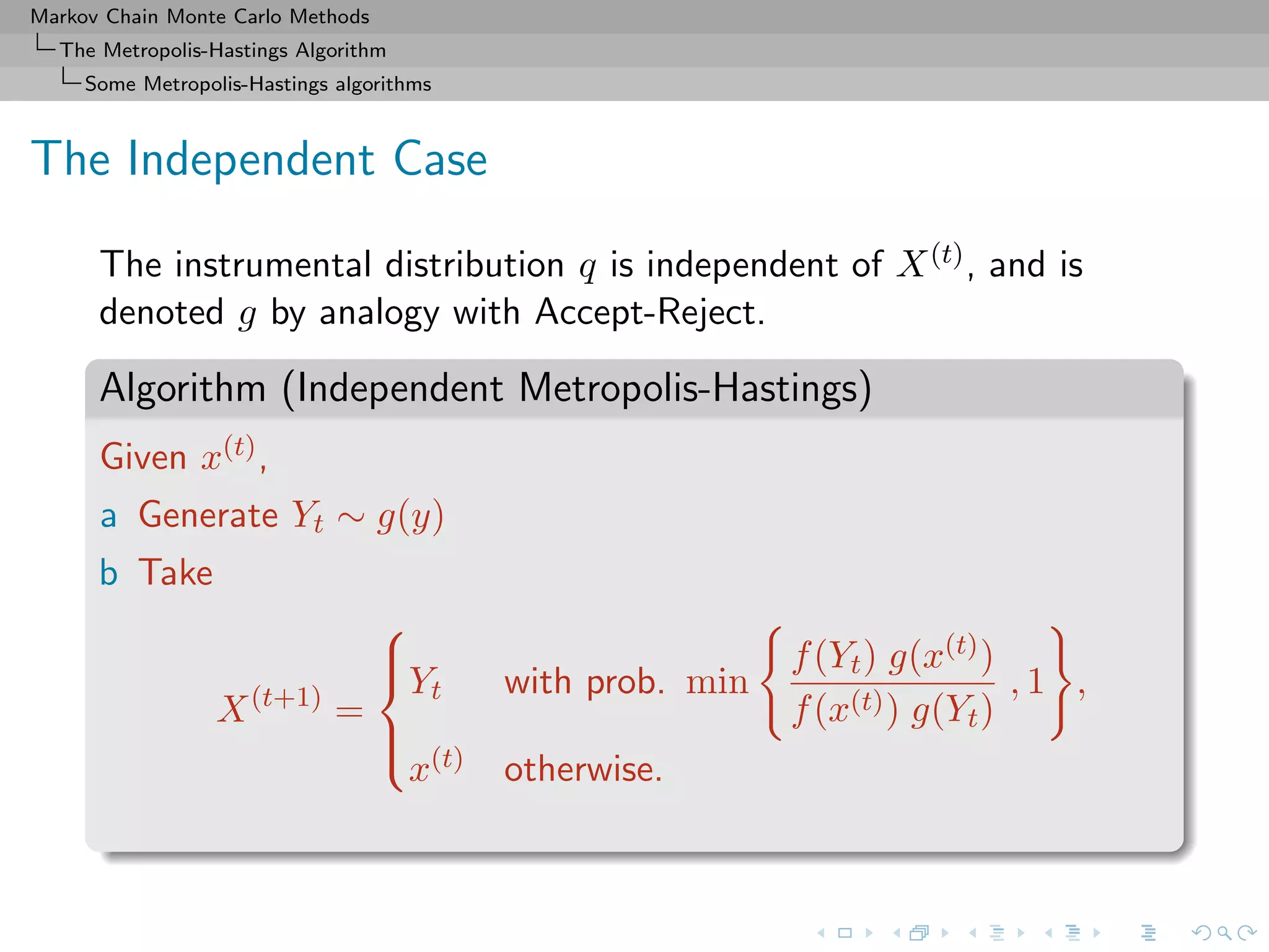
called the instrumental (or proposal)
distribution
[Metropolis & al., 1953]](https://image.slidesharecdn.com/cirm-181022142714/75/short-course-at-CIRM-Bayesian-Masterclass-October-2018-9-2048.jpg)
![Markov Chain Monte Carlo Methods
The Metropolis-Hastings Algorithm
Some Metropolis-Hastings algorithms
Properties
The resulting sample is not iid but there exist strong convergence
properties:
Theorem (Ergodicity)
The algorithm produces a uniformly ergodic chain if there exists a
constant M such that
f(x) ≤ Mg(x) , x ∈ supp f.
In this case,
Kn
(x, ·) − f TV ≤ 1 −
1
M
n
.
[Mengersen & Tweedie, 1996]](https://image.slidesharecdn.com/cirm-181022142714/75/short-course-at-CIRM-Bayesian-Masterclass-October-2018-21-2048.jpg)
![Markov Chain Monte Carlo Methods
The Metropolis-Hastings Algorithm
Some Metropolis-Hastings algorithms
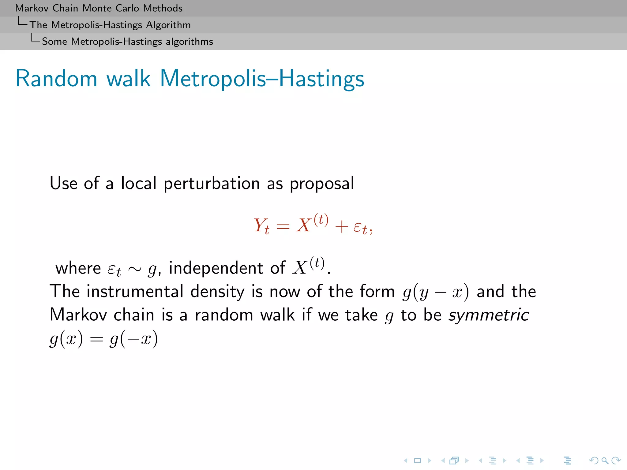
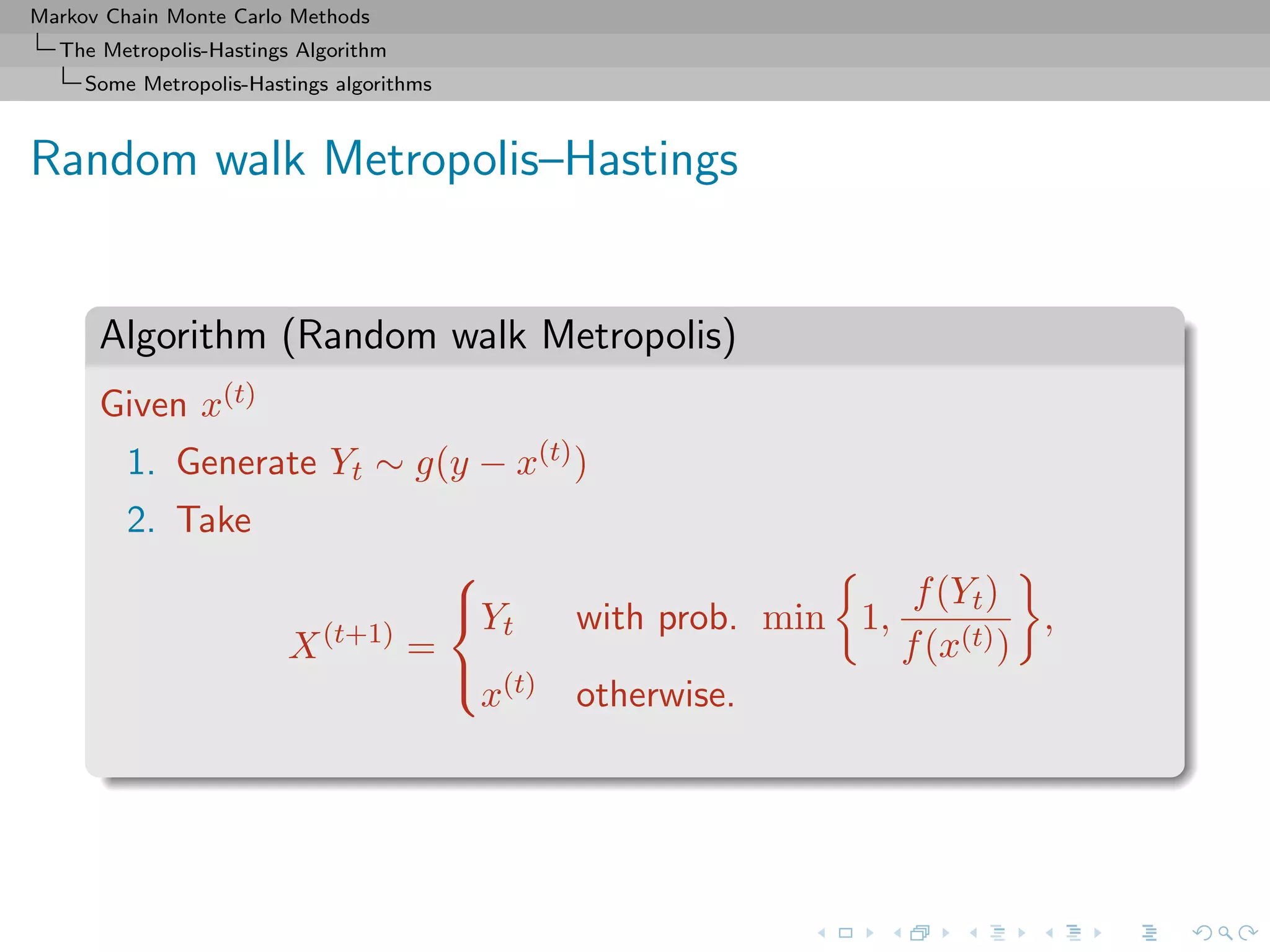
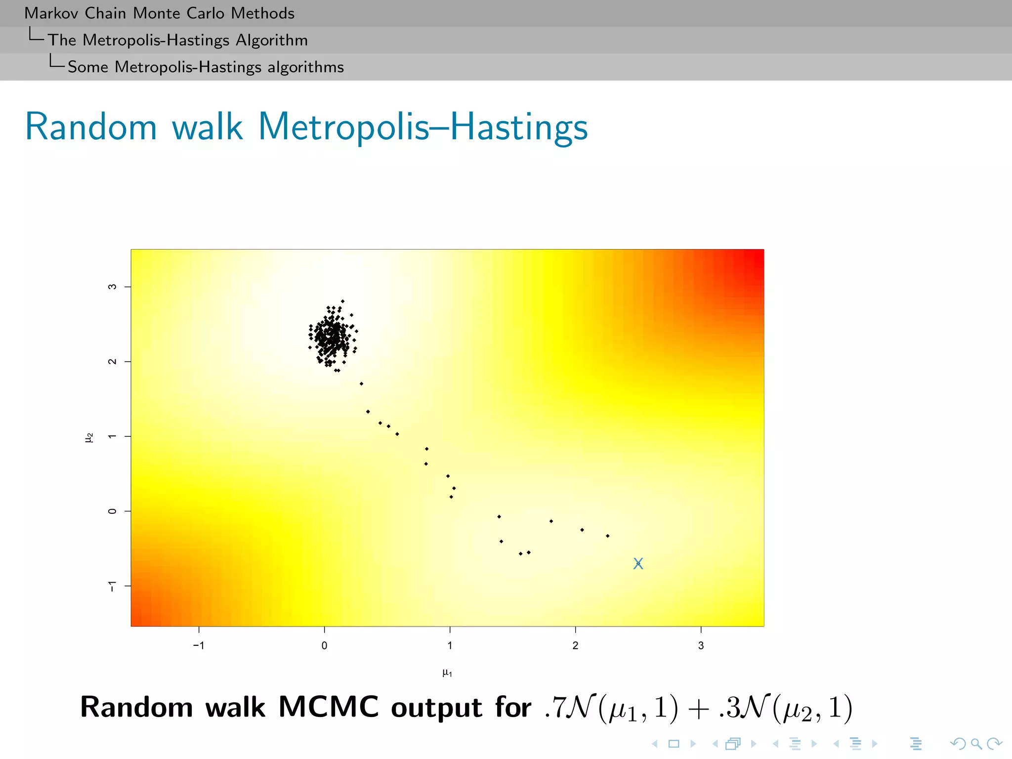
Random walk Metropolis–Hastings
Example (Random walk and normal target)
Generate N(0, 1) based on the uniform proposal [−δ, δ]
[Hastings (1970)]
The probability of acceptance is then
ρ(x(t)
, yt) = exp{(x(t)2
− y2
t )/2} ∧ 1.](https://image.slidesharecdn.com/cirm-181022142714/75/short-course-at-CIRM-Bayesian-Masterclass-October-2018-29-2048.jpg)
![Markov Chain Monte Carlo Methods
The Metropolis-Hastings Algorithm
Some Metropolis-Hastings algorithms
Random walk Metropolis–Hastings
p
theta
0.0 0.2 0.4 0.6 0.8 1.0
-1012
tau
theta
0.2 0.4 0.6 0.8 1.0 1.2
-1012
p
tau
0.0 0.2 0.4 0.6 0.8 1.0
0.20.40.60.81.01.2
-1 0 1 20.01.02.0
theta
0.2 0.4 0.6 0.8
024
tau
0.0 0.2 0.4 0.6 0.8 1.0
0123456
p
Random walk sampling (50000 iterations)
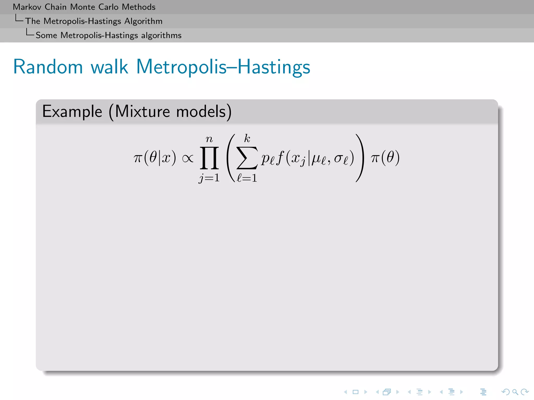
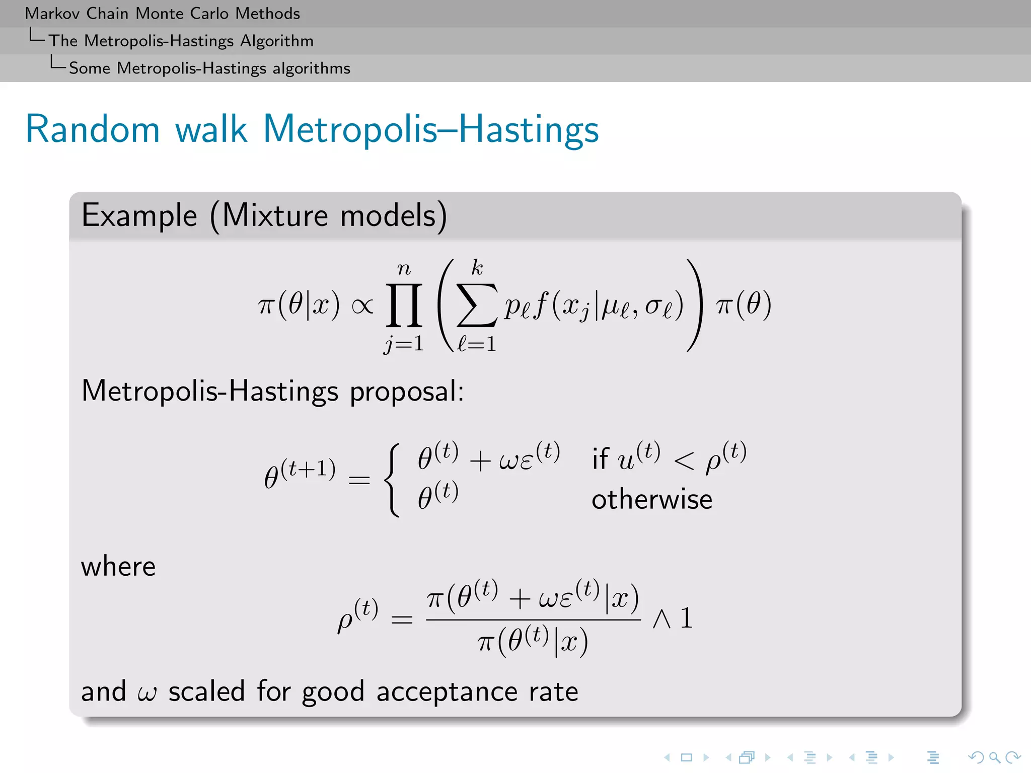
General case of a 3 component normal mixture
[Celeux & al., 2000]](https://image.slidesharecdn.com/cirm-181022142714/75/short-course-at-CIRM-Bayesian-Masterclass-October-2018-32-2048.jpg)
![Markov Chain Monte Carlo Methods
The Metropolis-Hastings Algorithm
Some Metropolis-Hastings algorithms
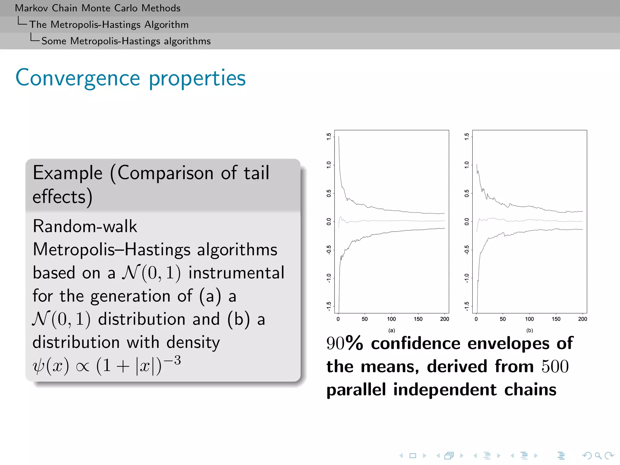
Convergence properties
Uniform ergodicity prohibited by random walk structure
At best, geometric ergodicity:
Theorem (Sufficient ergodicity)
For a symmetric density f, log-concave in the tails, and a positive
and symmetric density g, the chain (X(t)) is geometrically ergodic.
[Mengersen & Tweedie, 1996]
no tail effect](https://image.slidesharecdn.com/cirm-181022142714/75/short-course-at-CIRM-Bayesian-Masterclass-October-2018-38-2048.jpg)
![Markov Chain Monte Carlo Methods
The Metropolis-Hastings Algorithm
Some Metropolis-Hastings algorithms
Convergence properties
Example (Cauchy by normal)
Cauchy C (0, 1) target and Gaussian random walk proposal,
ξ ∼ N (ξ, σ2), with acceptance probability
1 + ξ2
1 + (ξ )2
∧ 1 ,
Overall fit of the Cauchy density by the histogram satisfactory, but
poor exploration of the tails: 99% quantile of C (0, 1) equal to 3,
but no simulation exceeds 14 out of 10, 000!
[Roberts & Tweedie, 2004]](https://image.slidesharecdn.com/cirm-181022142714/75/short-course-at-CIRM-Bayesian-Masterclass-October-2018-40-2048.jpg)
![Markov Chain Monte Carlo Methods
The Metropolis-Hastings Algorithm
Some Metropolis-Hastings algorithms
Convergence properties
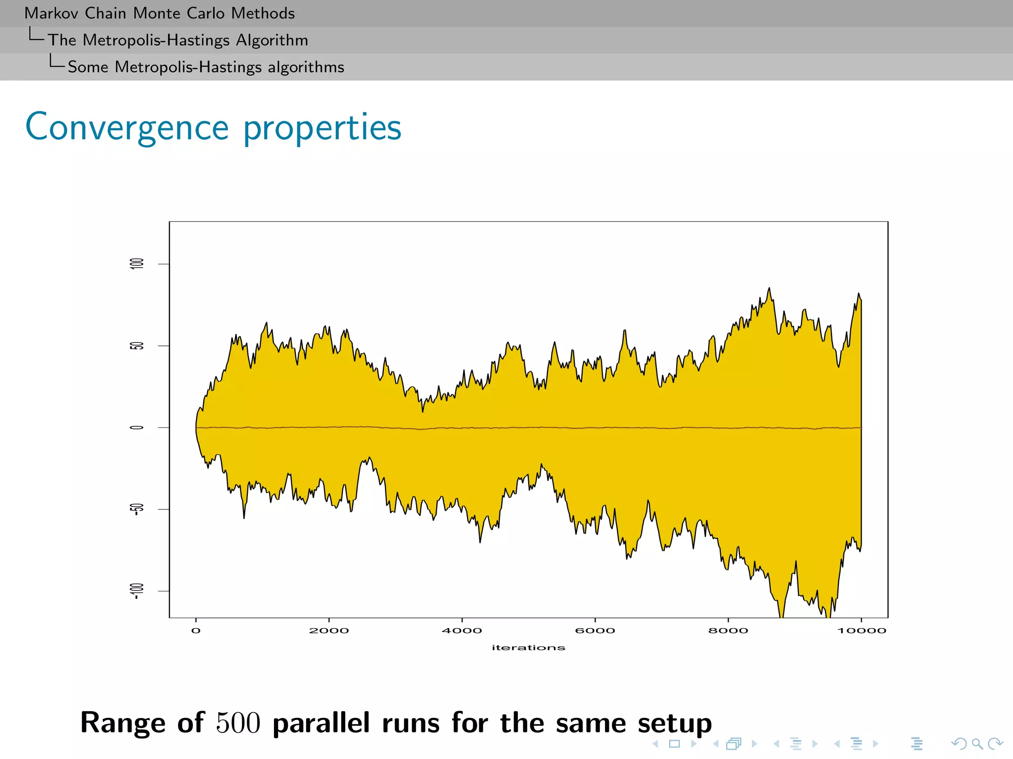
Again, lack of geometric ergodicity!
[Mengersen & Tweedie, 1996]
Slow convergence shown by the non-stable range after 10, 000
iterations.
Density
−5 0 5
0.000.050.100.150.200.250.300.35](https://image.slidesharecdn.com/cirm-181022142714/75/short-course-at-CIRM-Bayesian-Masterclass-October-2018-41-2048.jpg)
![Markov Chain Monte Carlo Methods
The Metropolis-Hastings Algorithm
Some Metropolis-Hastings algorithms
Comments
[CLT, Rosenthal’s inequality...] h-ergodicity implies CLT
for additive (possibly unbounded) functionals of the chain,
Rosenthal’s inequality and so on...
[Control of the moments of the return-time] The
condition implies (because h ≥ 1) that
sup
x∈C
Ex[r0(τC)] ≤ sup
x∈C
Ex
τC −1
k=0
r(k)h(Xk) < ∞,
where r0(n) = n
l=0 r(l) Can be used to derive bounds for
the coupling time, an essential step to determine computable
bounds, using coupling inequalities
[Roberts & Tweedie, 1998; Fort & Moulines, 2000]](https://image.slidesharecdn.com/cirm-181022142714/75/short-course-at-CIRM-Bayesian-Masterclass-October-2018-43-2048.jpg)
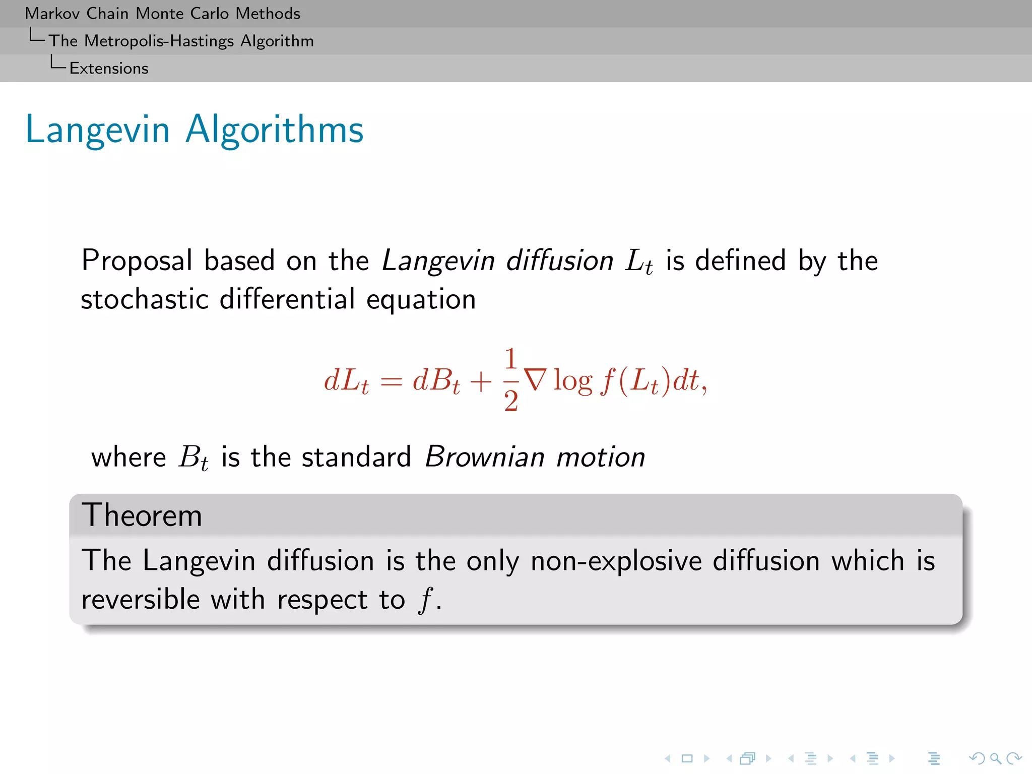
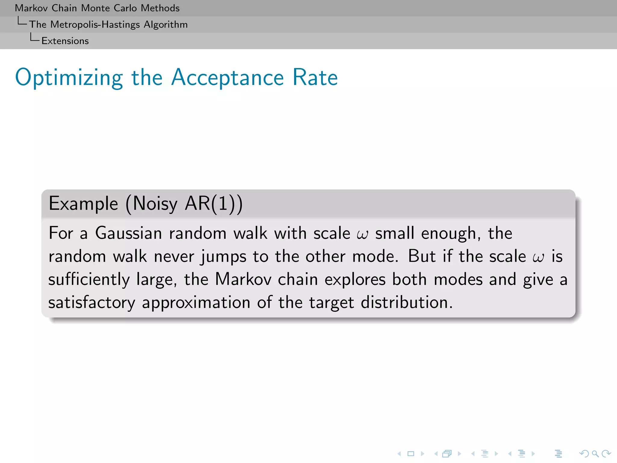
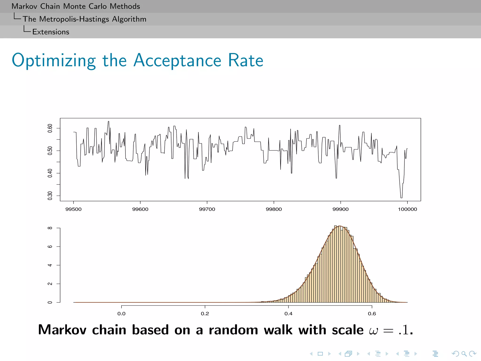
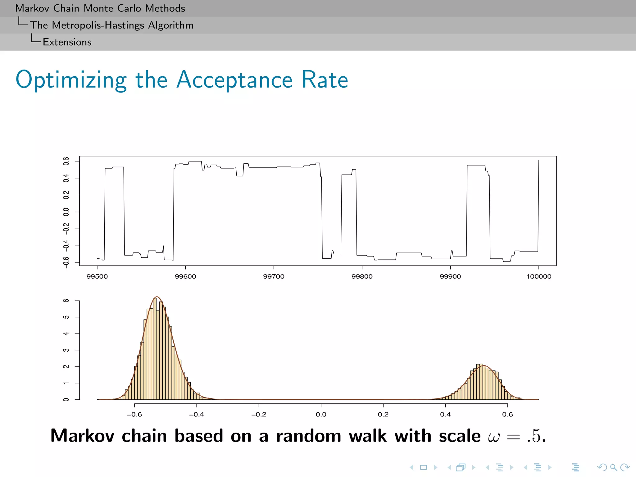
![Markov Chain Monte Carlo Methods
The Metropolis-Hastings Algorithm
Extensions
MH correction (MALA)
Accept the new value Yt with probability
f(Yt)
f(x(t))
·
exp − Yt − x(t) − σ2
2 log f(x(t))
2
2σ2
exp − x(t) − Yt − σ2
2 log f(Yt)
2
2σ2
∧ 1 .
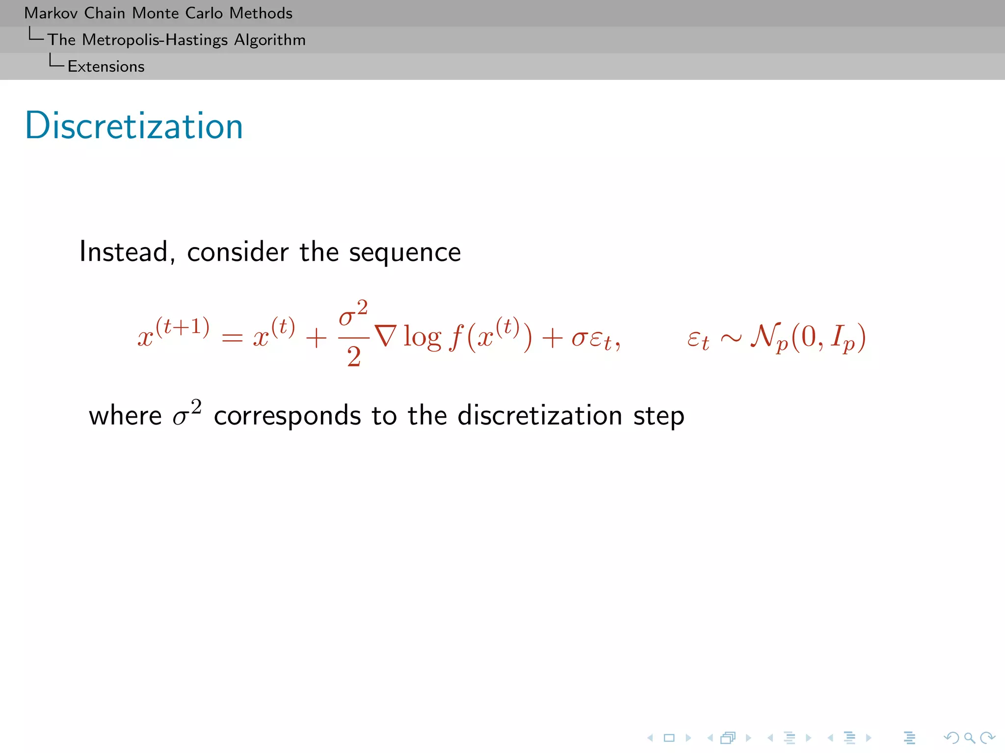
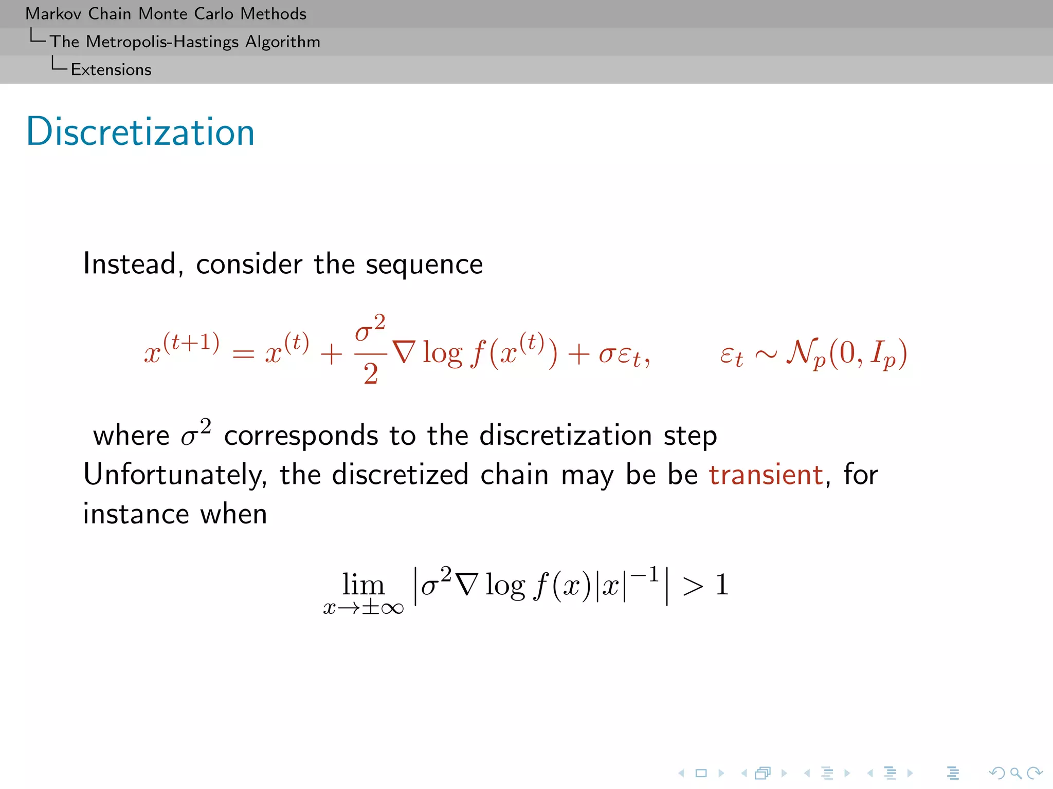
Choice of the scaling factor σ
Should lead to an acceptance rate of 0.574 to achieve optimal
convergence rates (when the components of x are uncorrelated)
[Roberts & Rosenthal, 1998]](https://image.slidesharecdn.com/cirm-181022142714/75/short-course-at-CIRM-Bayesian-Masterclass-October-2018-48-2048.jpg)

![Markov Chain Monte Carlo Methods
The Metropolis-Hastings Algorithm
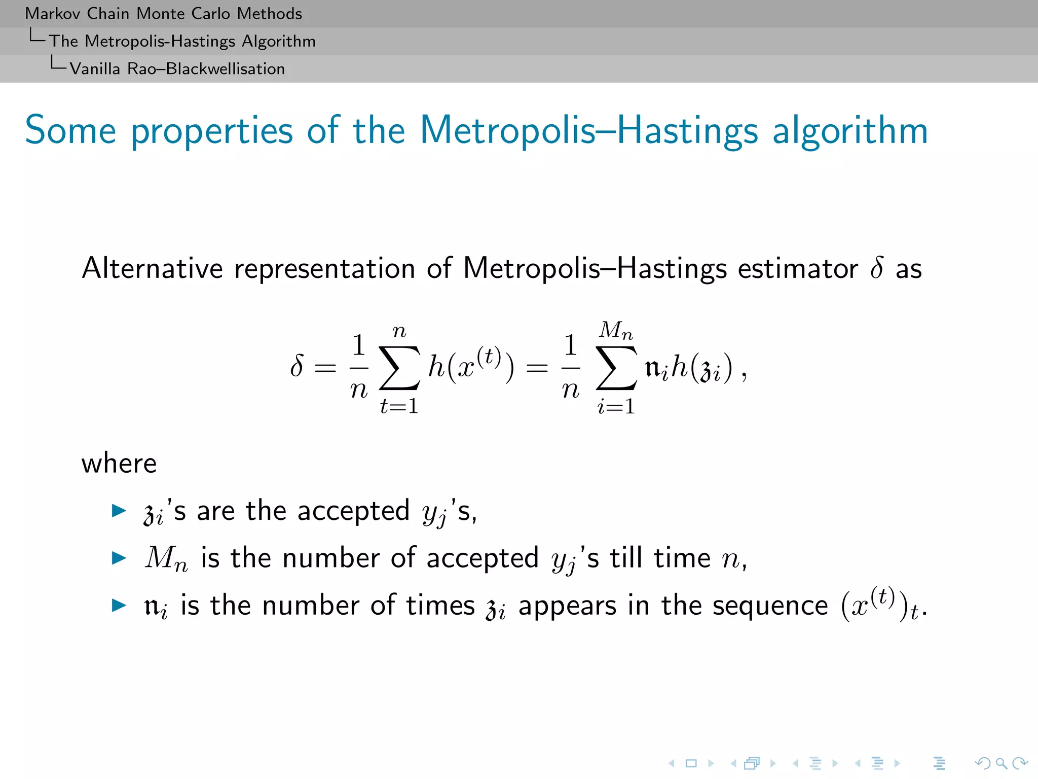
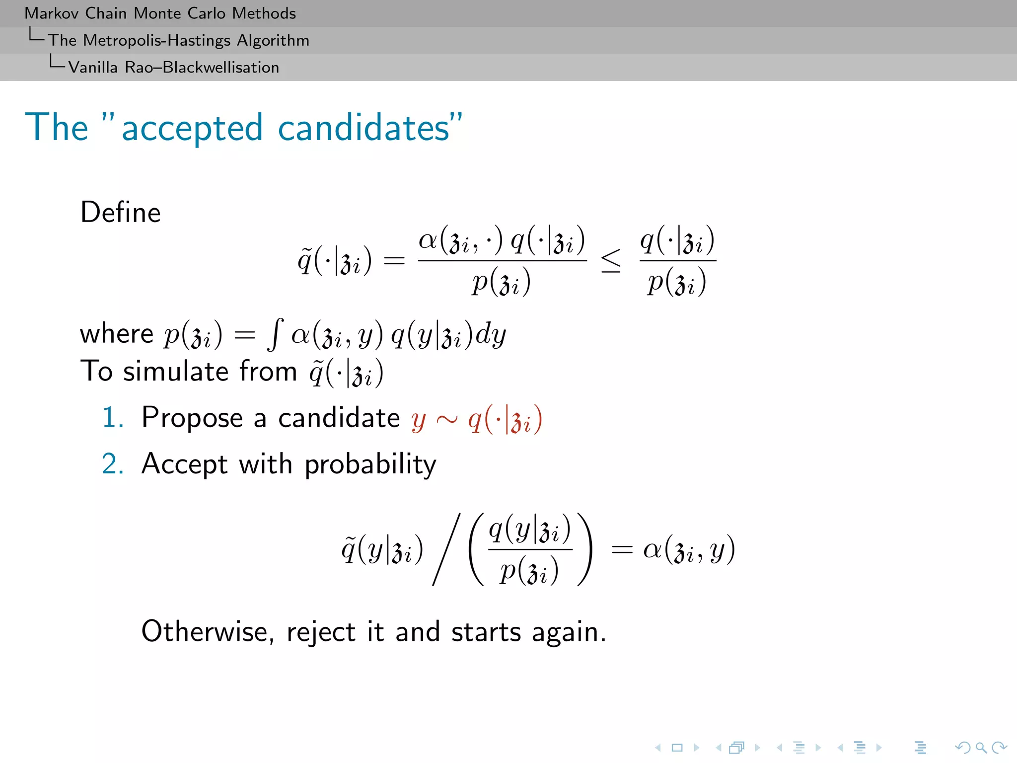
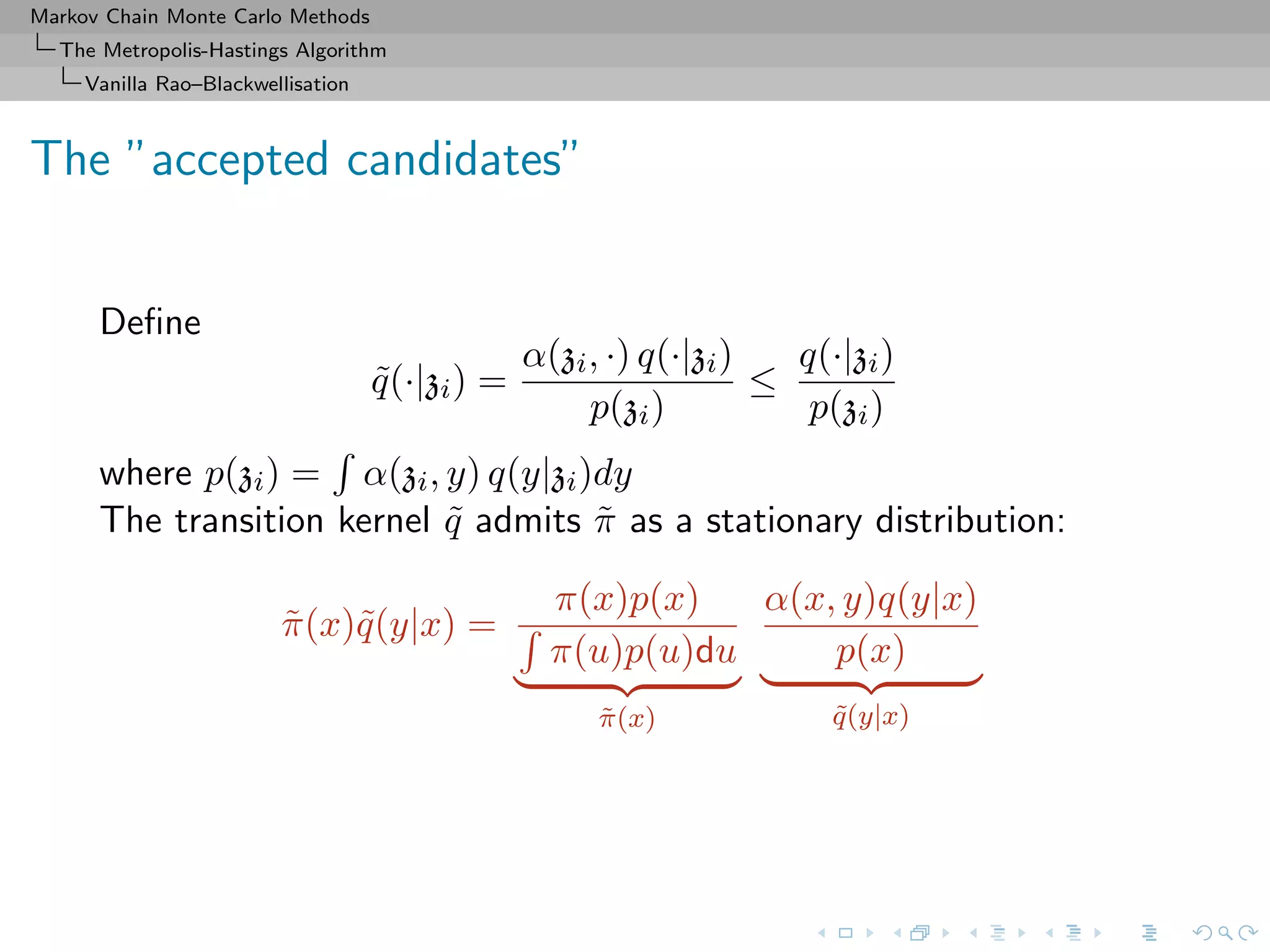
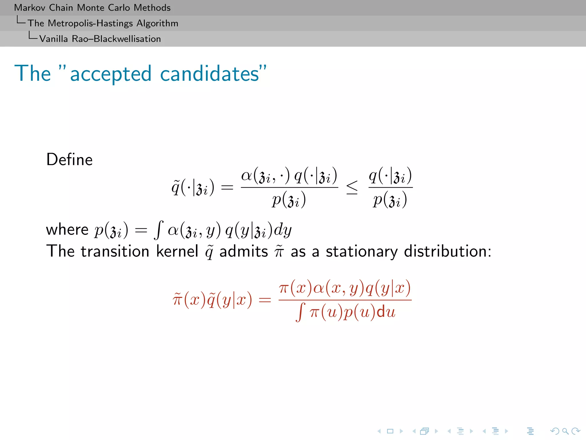
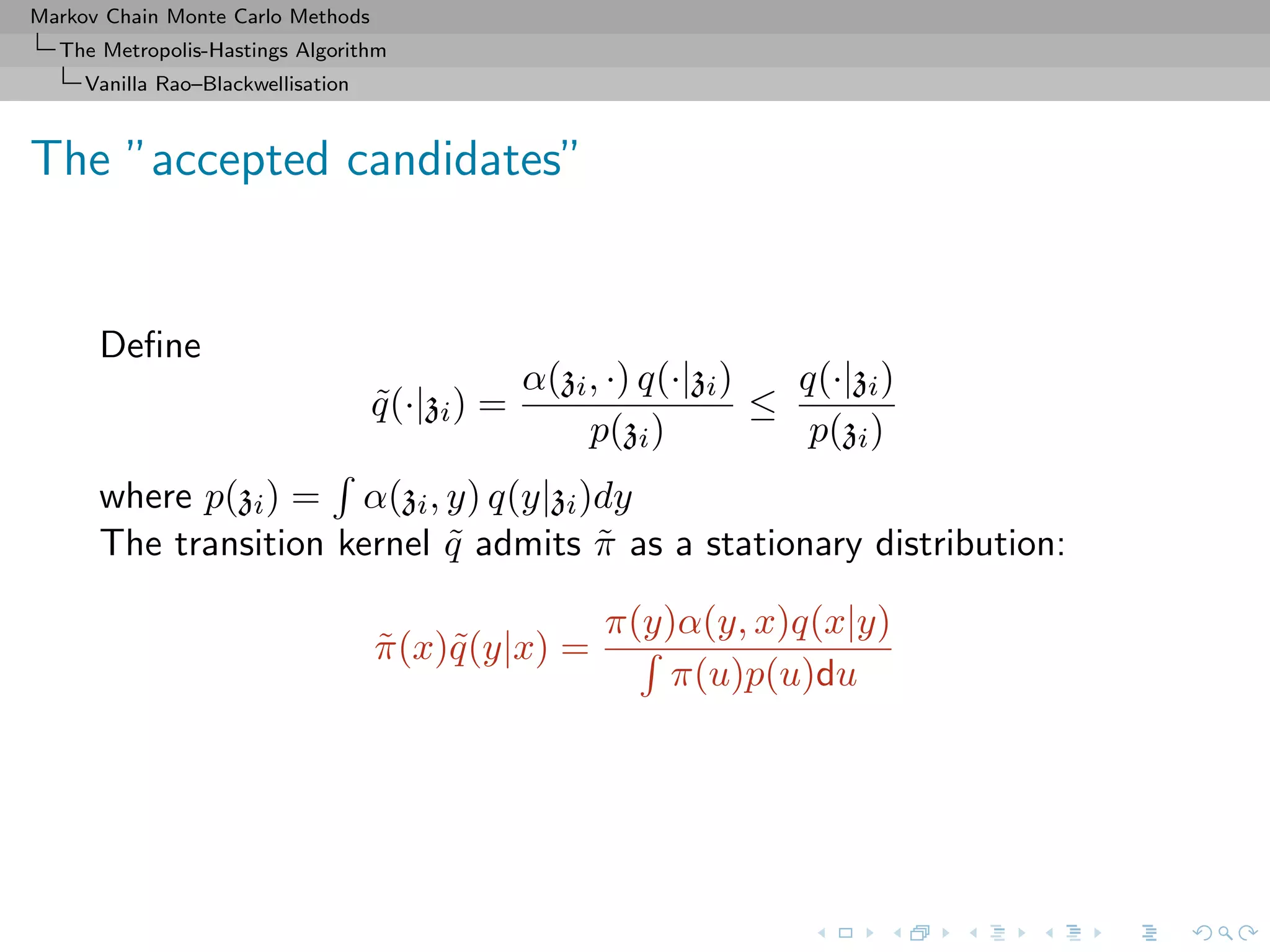
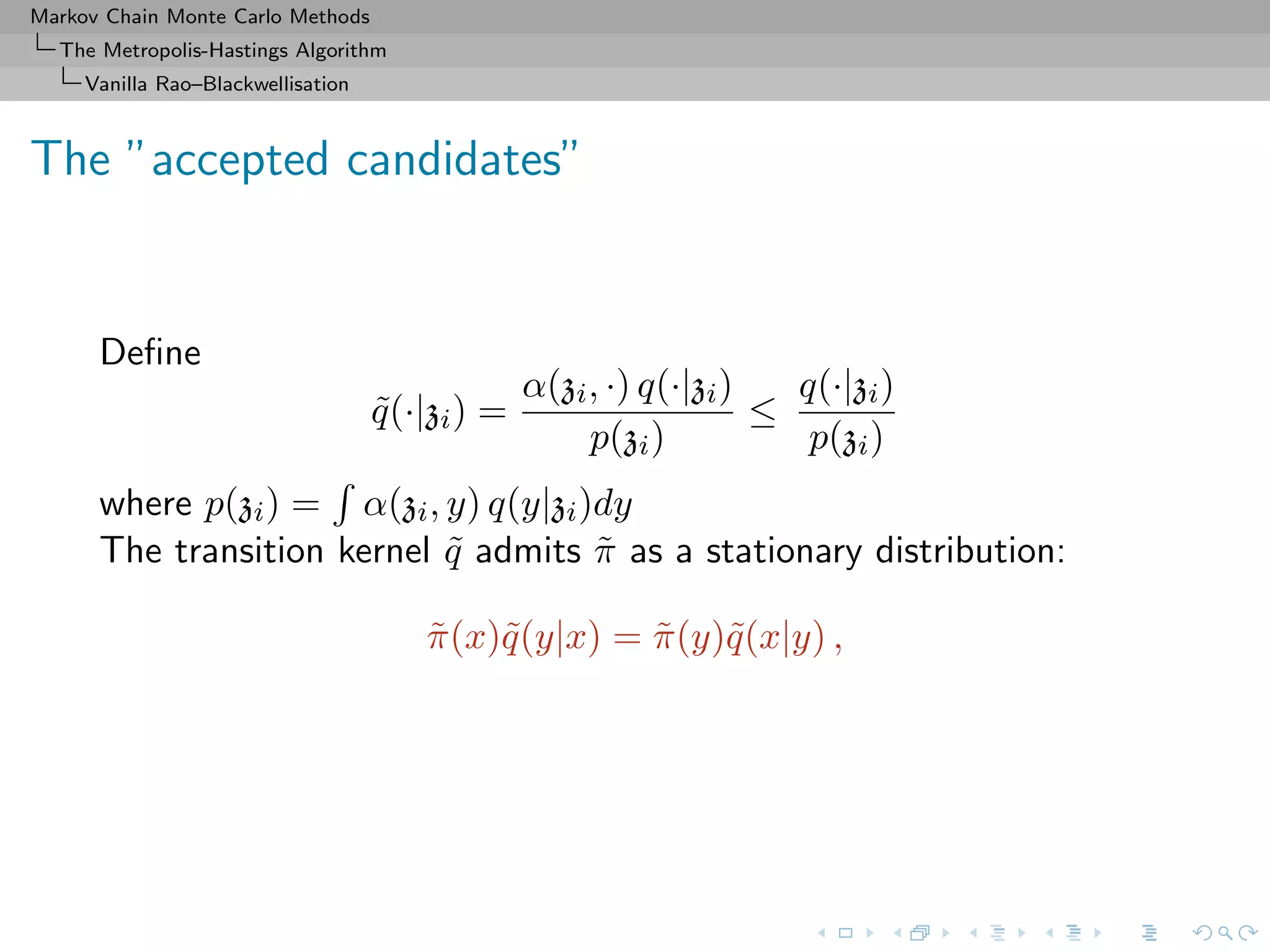
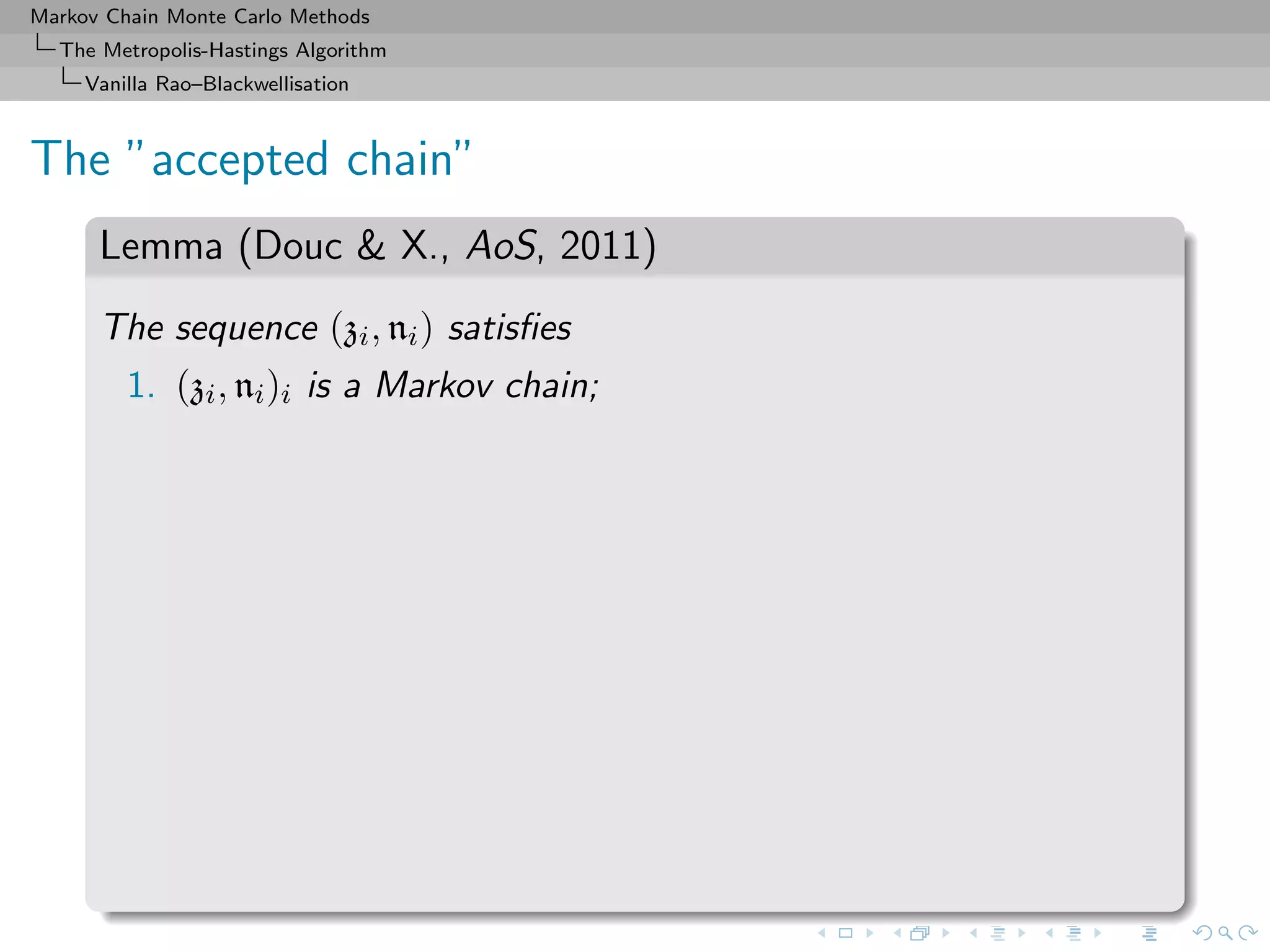
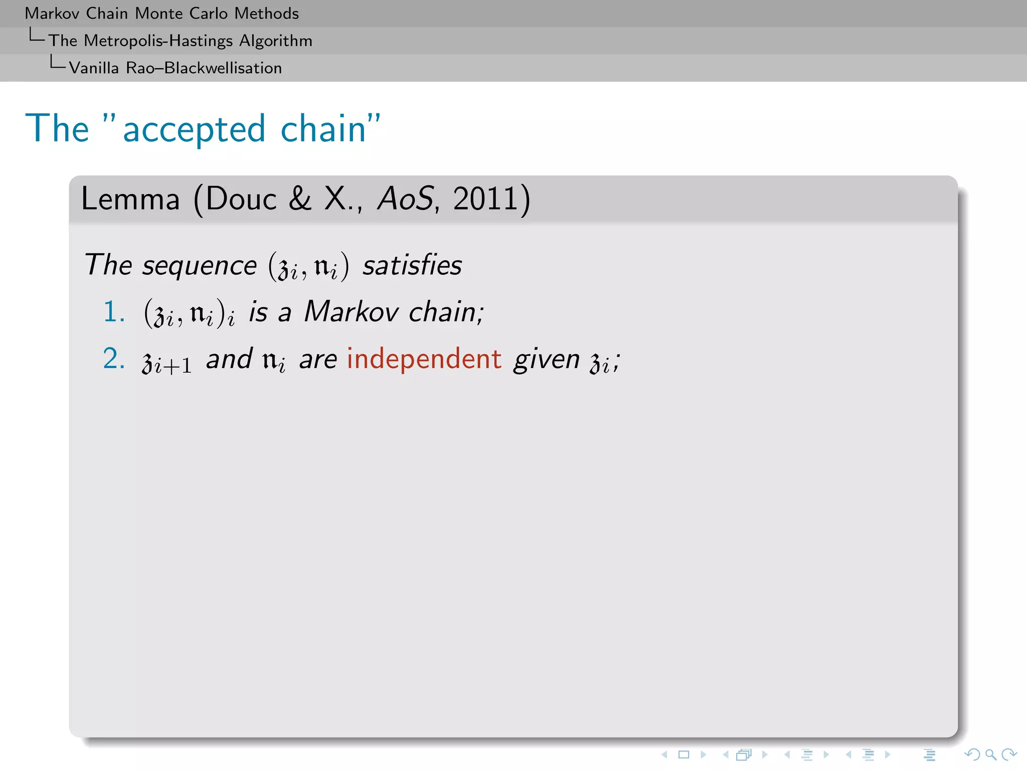
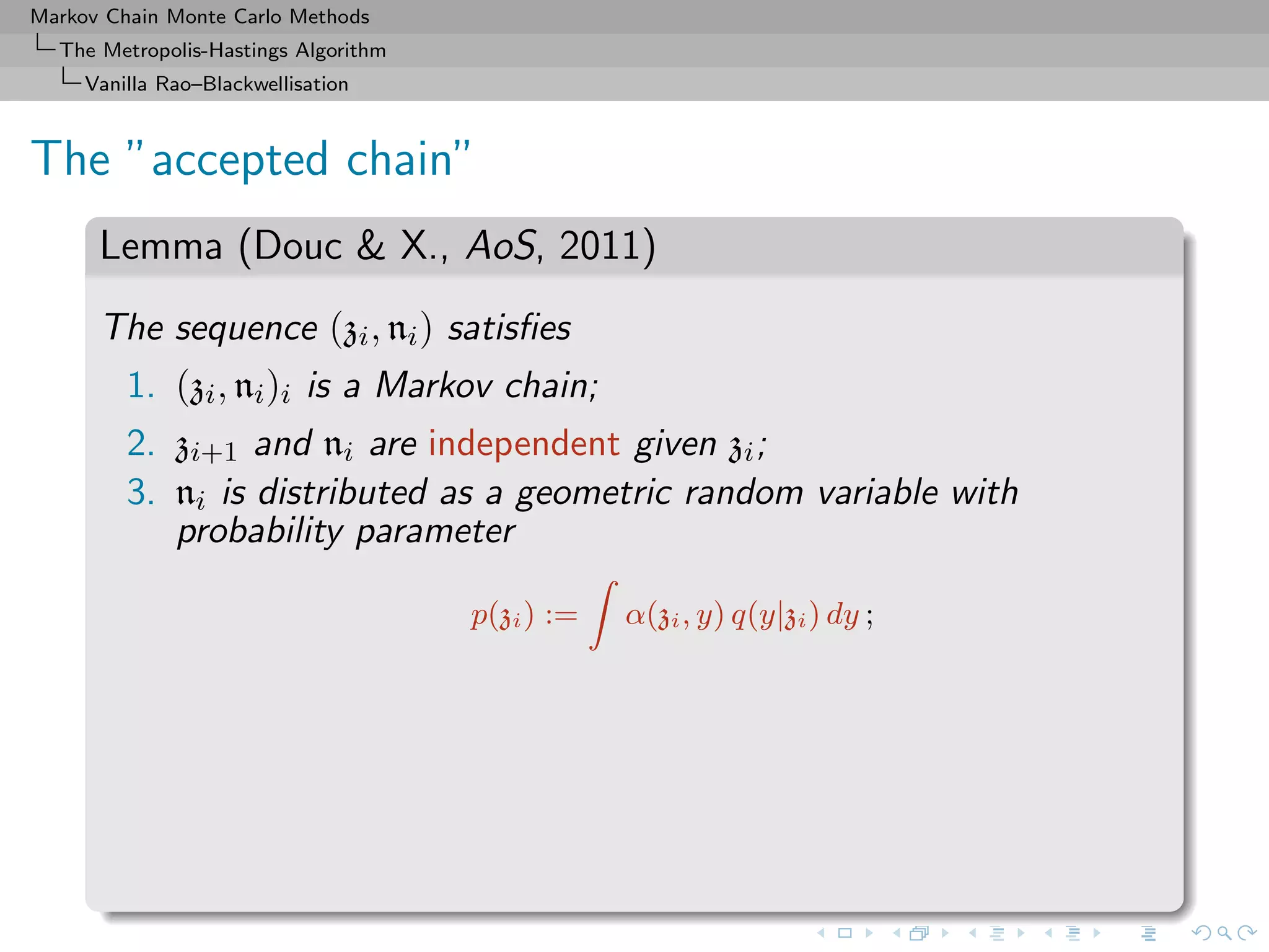
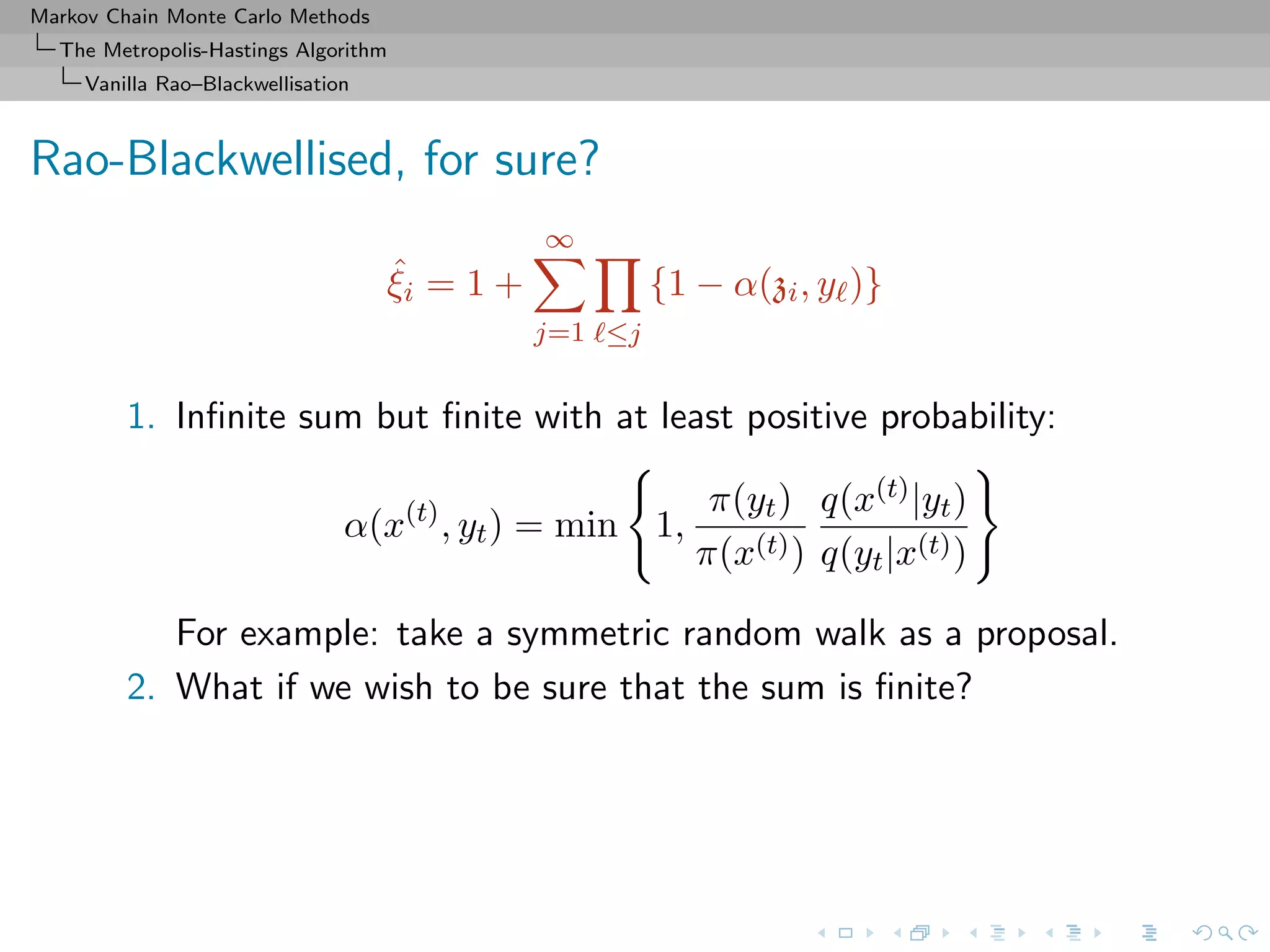
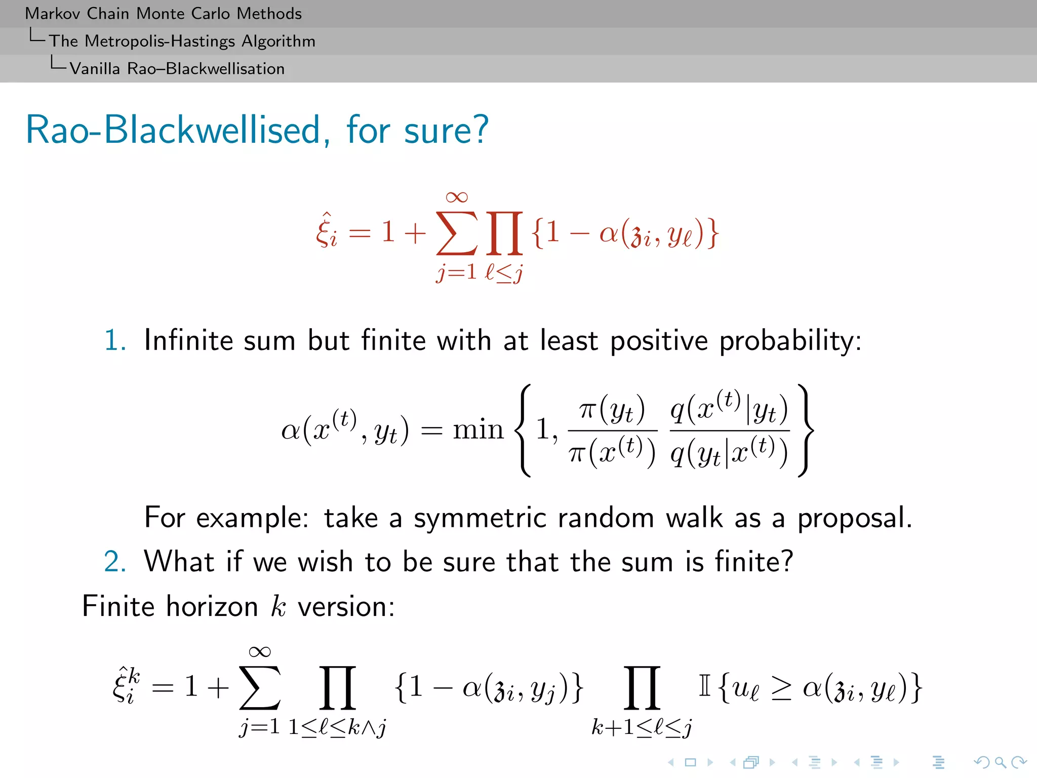
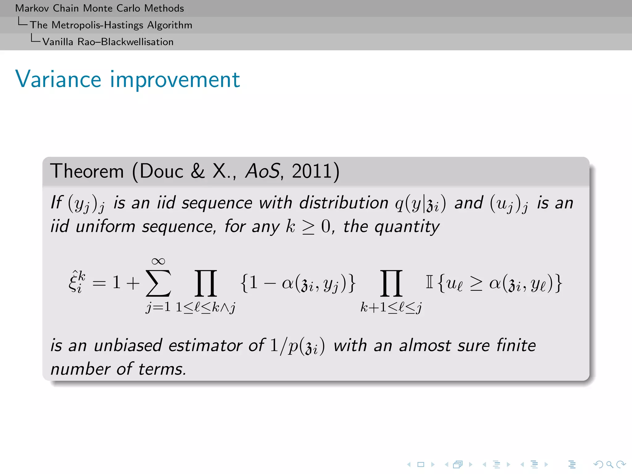
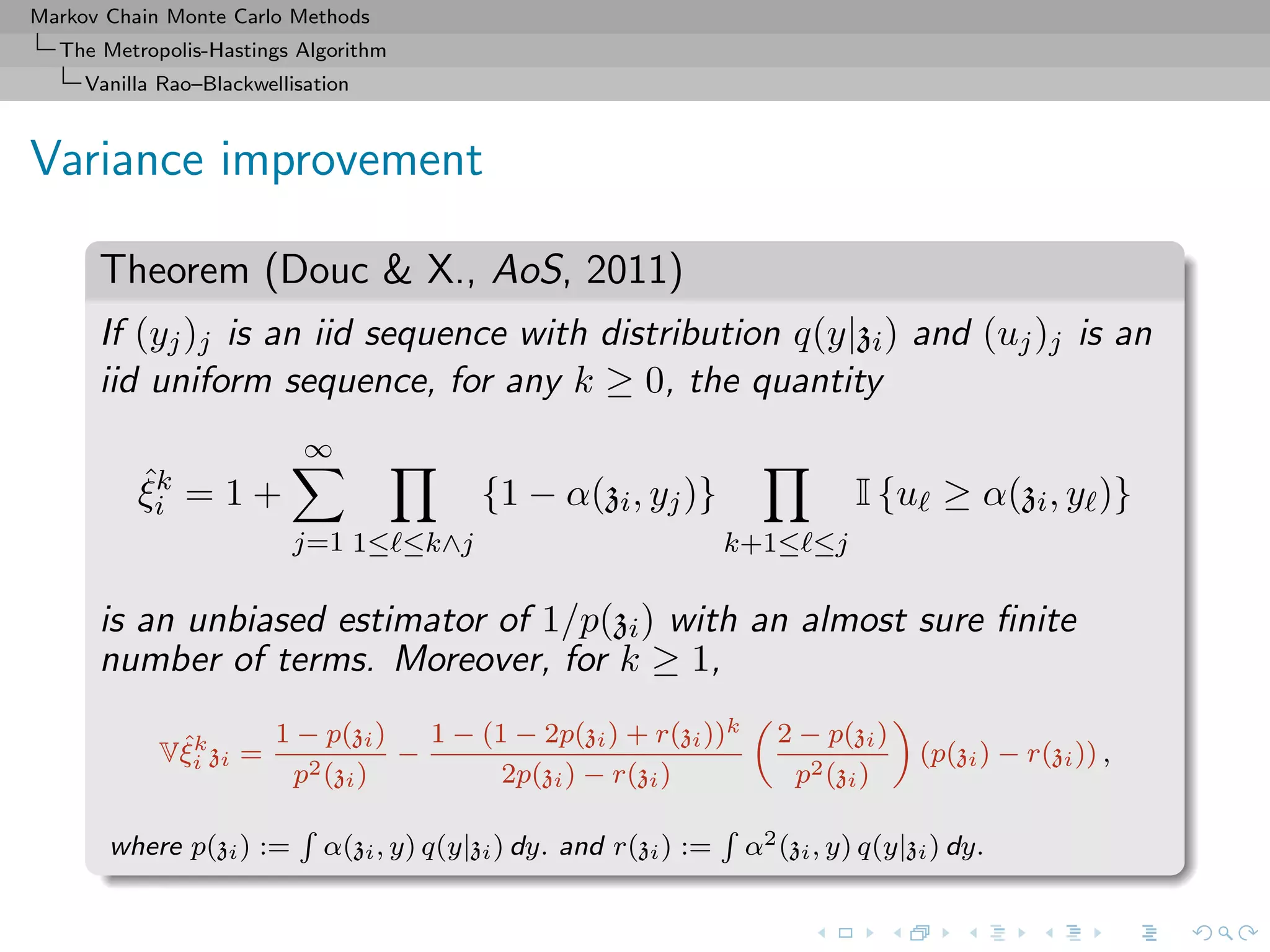
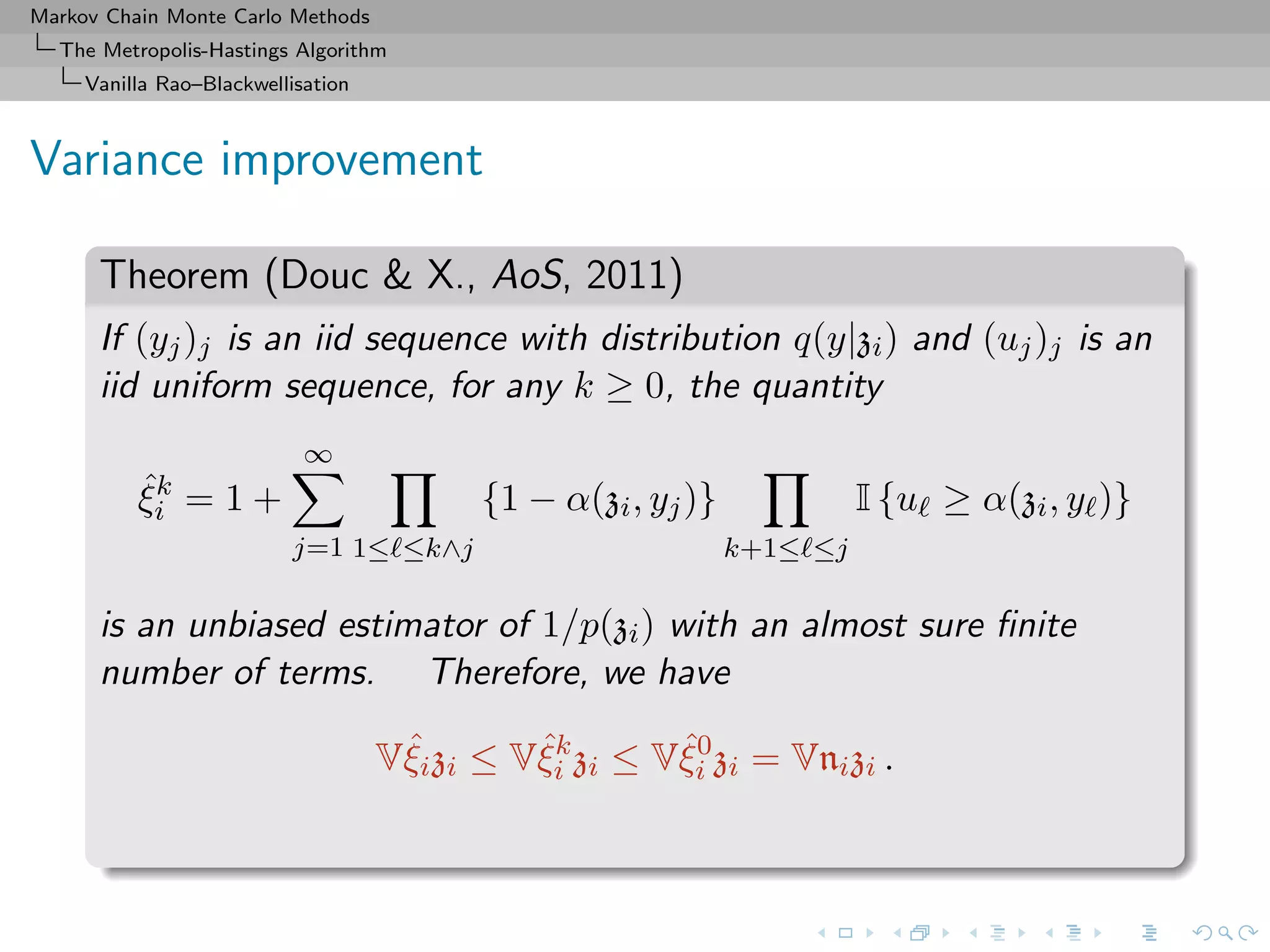
Vanilla Rao–Blackwellisation
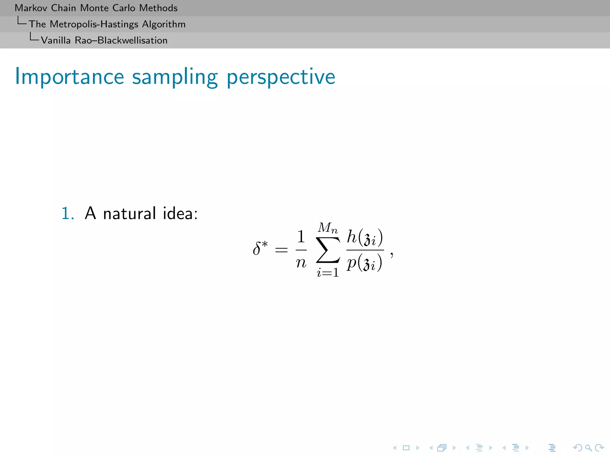
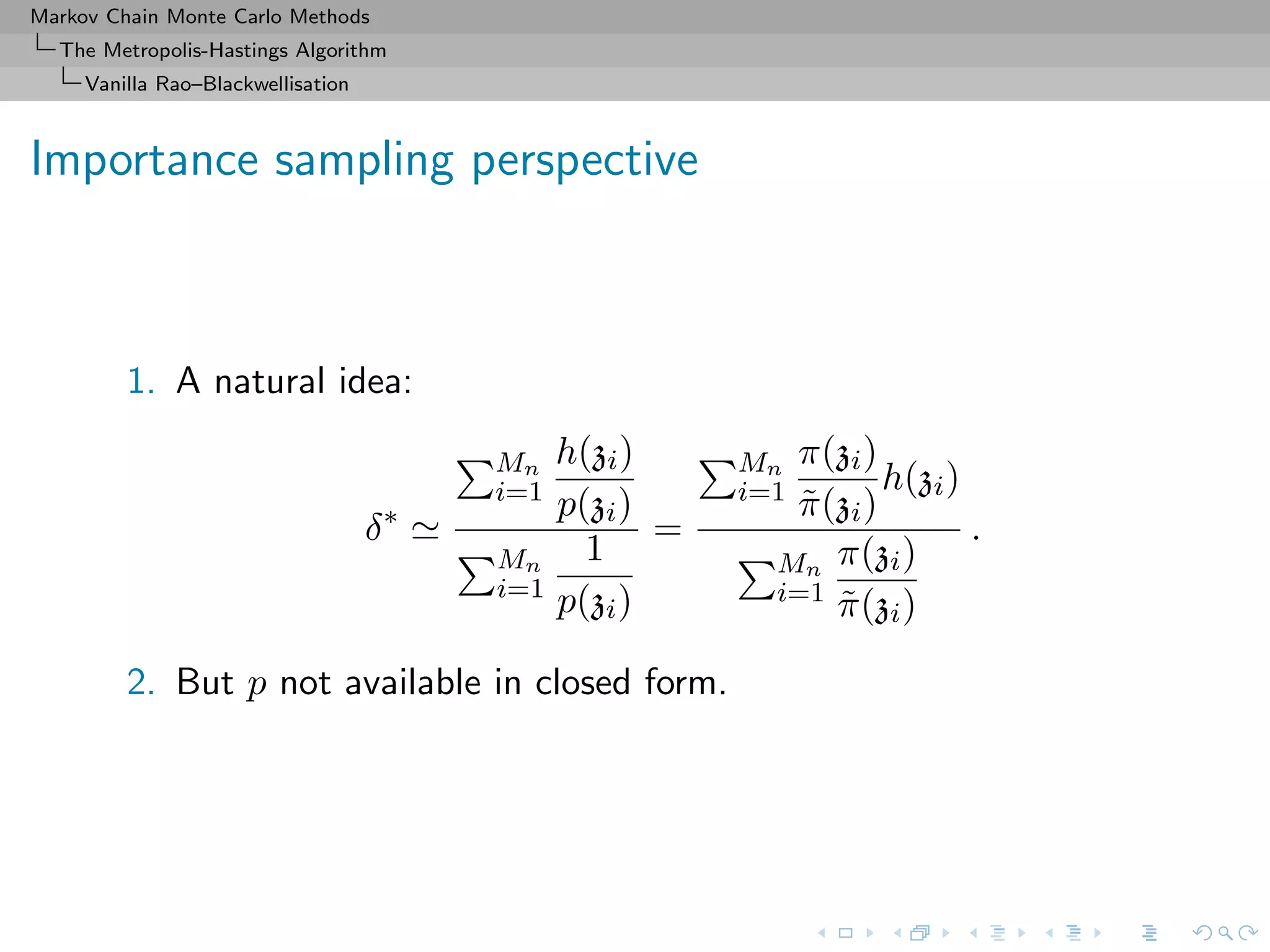
Importance sampling perspective
1. A natural idea:
δ∗
Mn
i=1
h(zi)
p(zi)
Mn
i=1
1
p(zi)
=
Mn
i=1
π(zi)
˜π(zi)
h(zi)
Mn
i=1
π(zi)
˜π(zi)
.
2. But p not available in closed form.
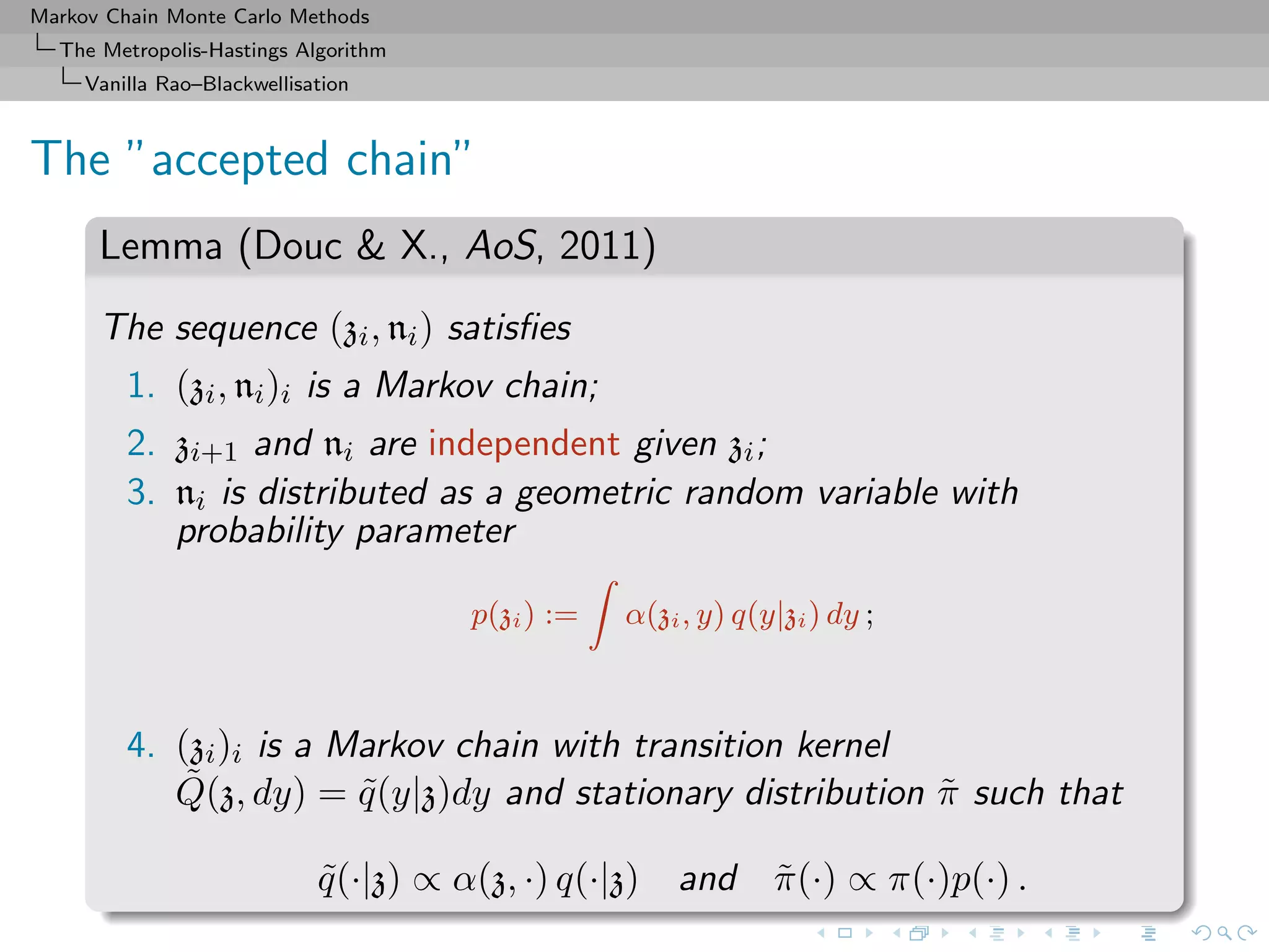
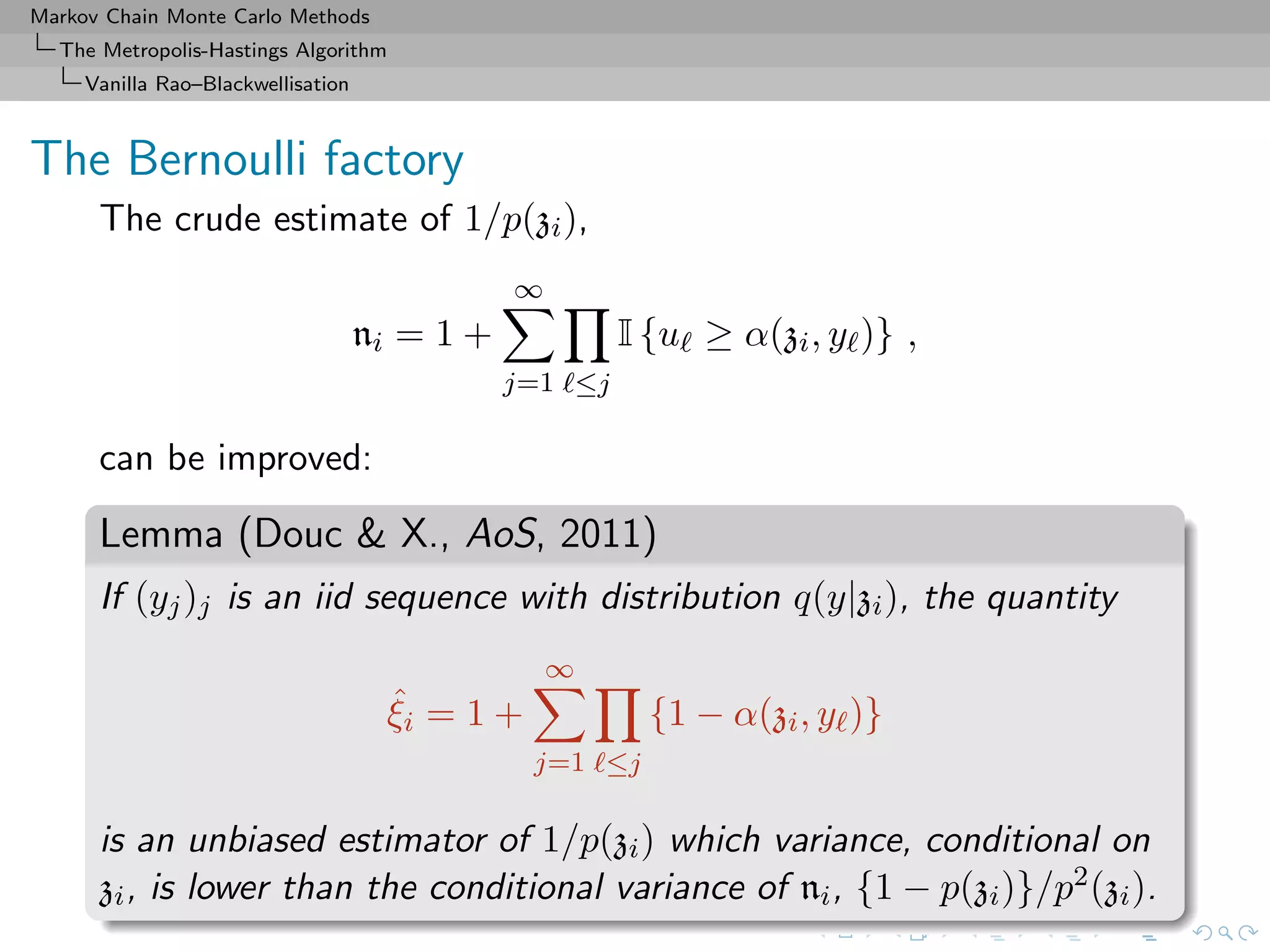
3. The geometric ni is the replacement, an obvious solution that
is used in the original Metropolis–Hastings estimate since
E[ni] = 1/p(zi).](https://image.slidesharecdn.com/cirm-181022142714/75/short-course-at-CIRM-Bayesian-Masterclass-October-2018-66-2048.jpg)
![Markov Chain Monte Carlo Methods
The Metropolis-Hastings Algorithm
Delayed acceptance
The “Big Data” plague
Simulation from posterior with largesample size n
Computing time at least of order O(n)
solutions using likelihood decomposition
n
i=1
(θ|xi)
and handling subsets on different processors (CPU), graphical
units (GPU), or computers
[Scott et al., 2013, Korattikara et al., 2013]
no consensus on method of choice, with instabilities from
removing most prior input and uncalibrated approximations
[Neiswanger et al., 2013]](https://image.slidesharecdn.com/cirm-181022142714/75/short-course-at-CIRM-Bayesian-Masterclass-October-2018-73-2048.jpg)
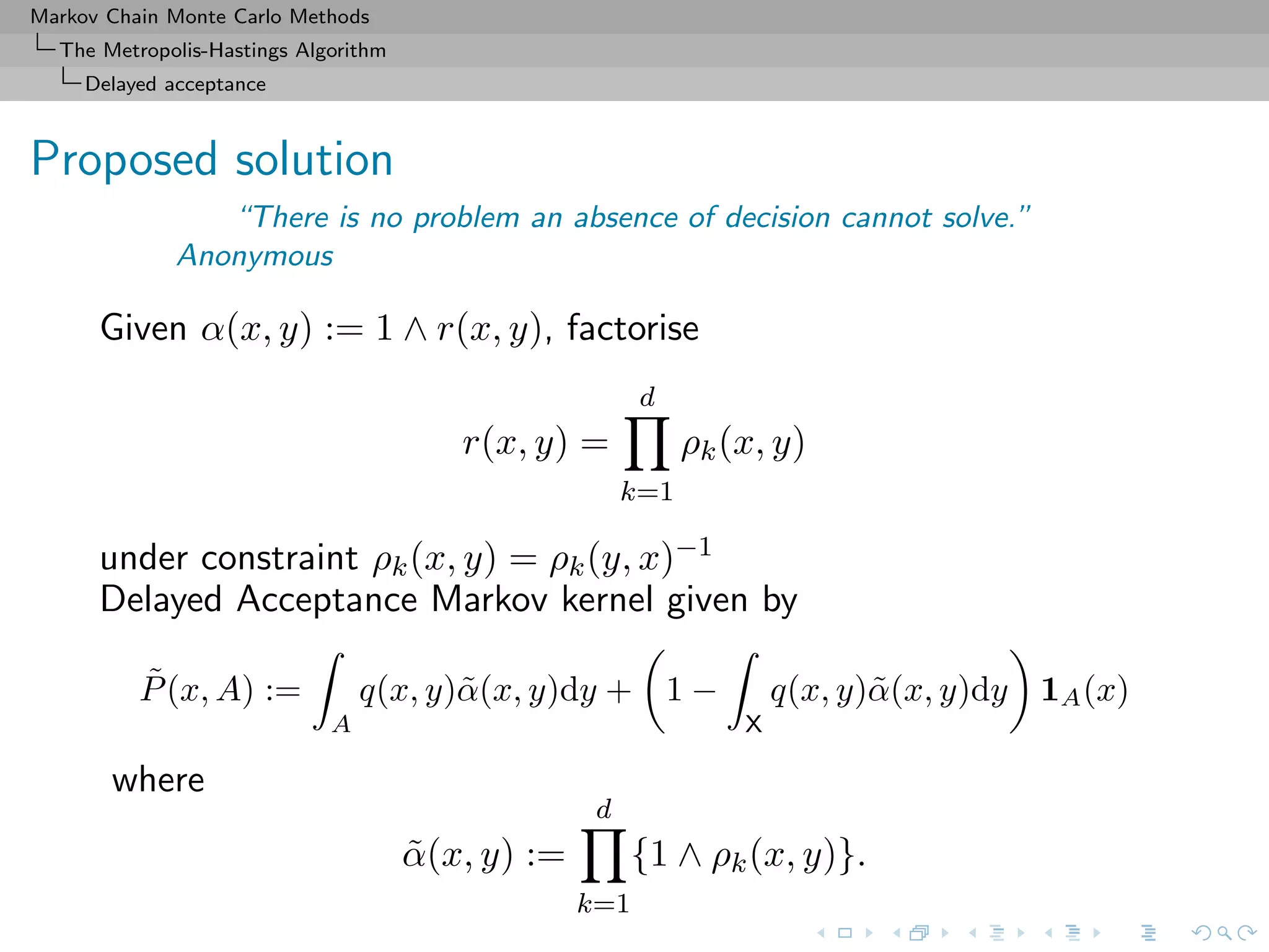
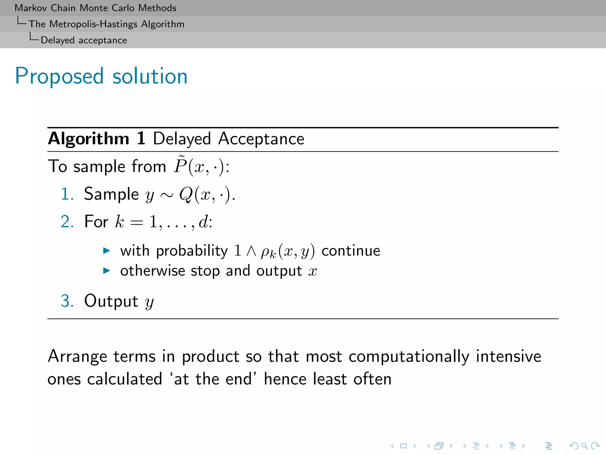
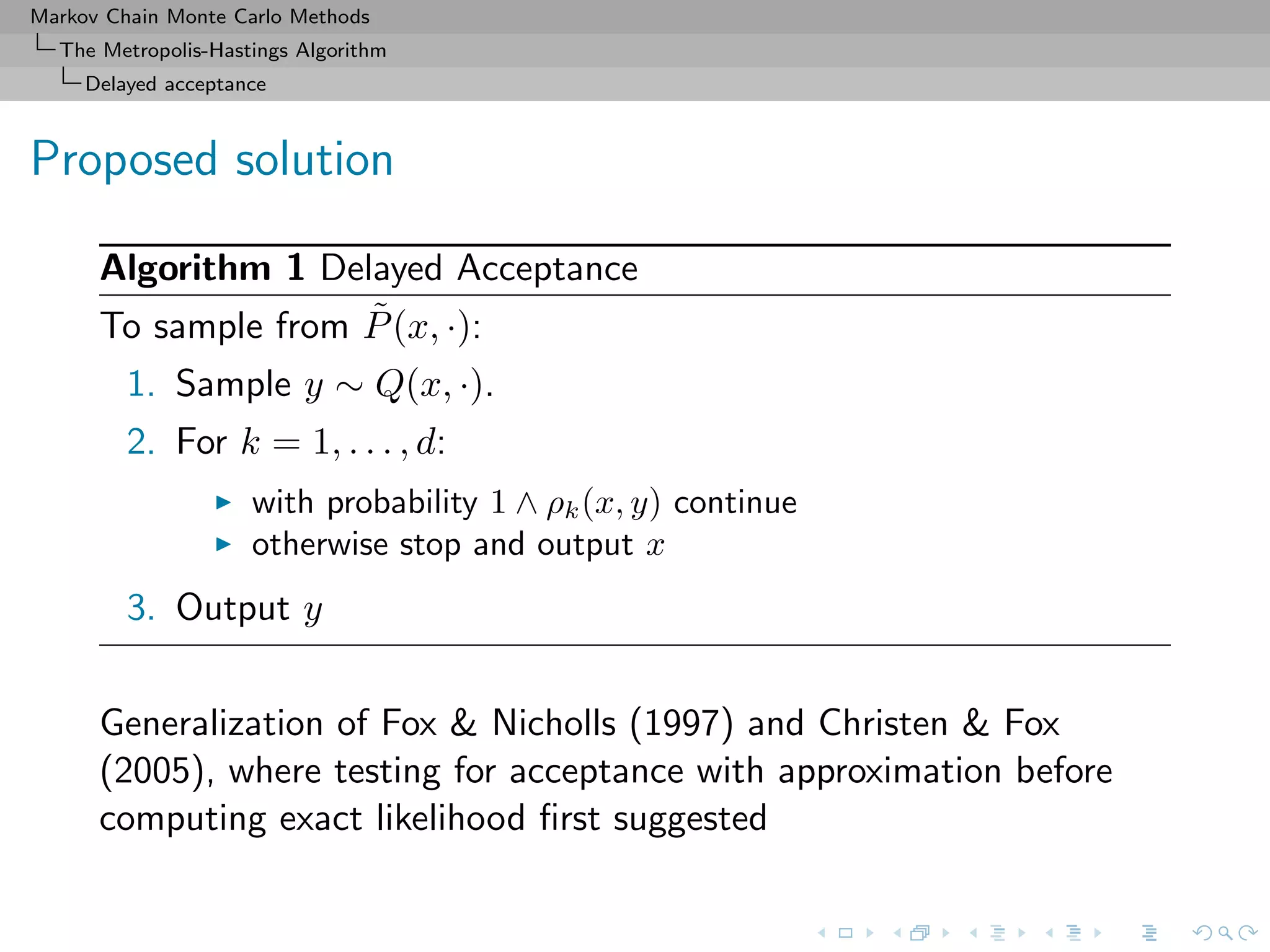
![Markov Chain Monte Carlo Methods
The Metropolis-Hastings Algorithm
Delayed acceptance
The “Big Data” plague
Delayed Acceptance intended for likelihoods or priors, but
not a clear solution for “Big Data” problems
1. all product terms must be computed
2. all terms previously computed either stored for future
comparison or recomputed
3. sequential approach limits parallel gains...
4. ...unless prefetching scheme added to delays
[Strid (2010)]](https://image.slidesharecdn.com/cirm-181022142714/75/short-course-at-CIRM-Bayesian-Masterclass-October-2018-77-2048.jpg)
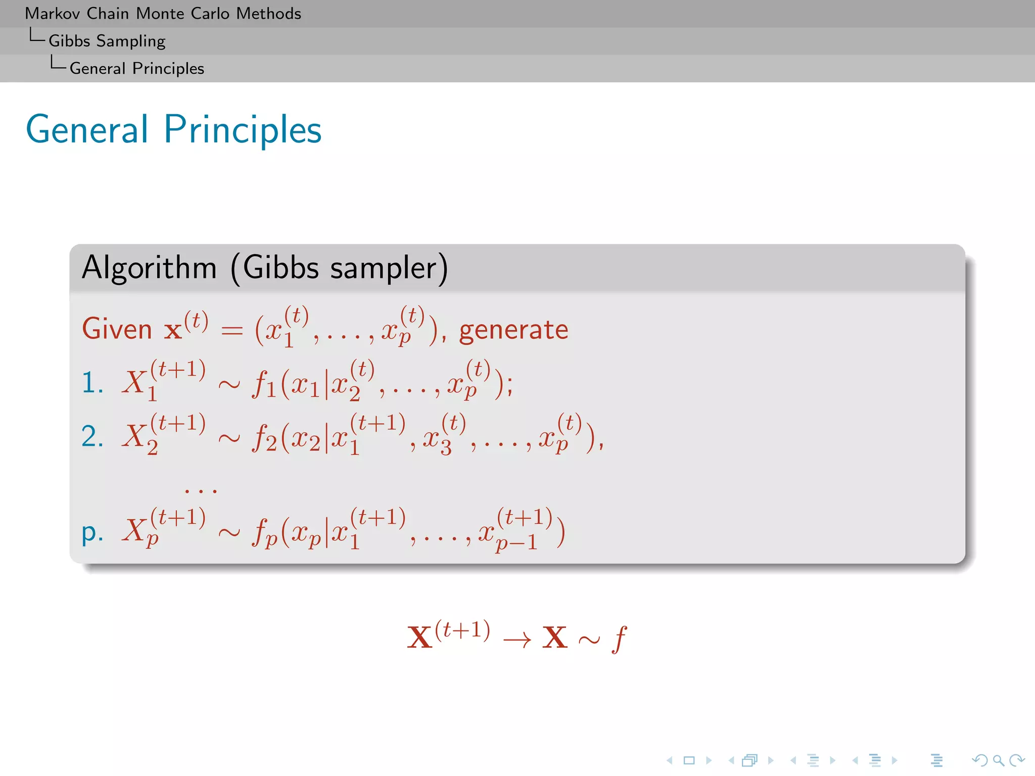
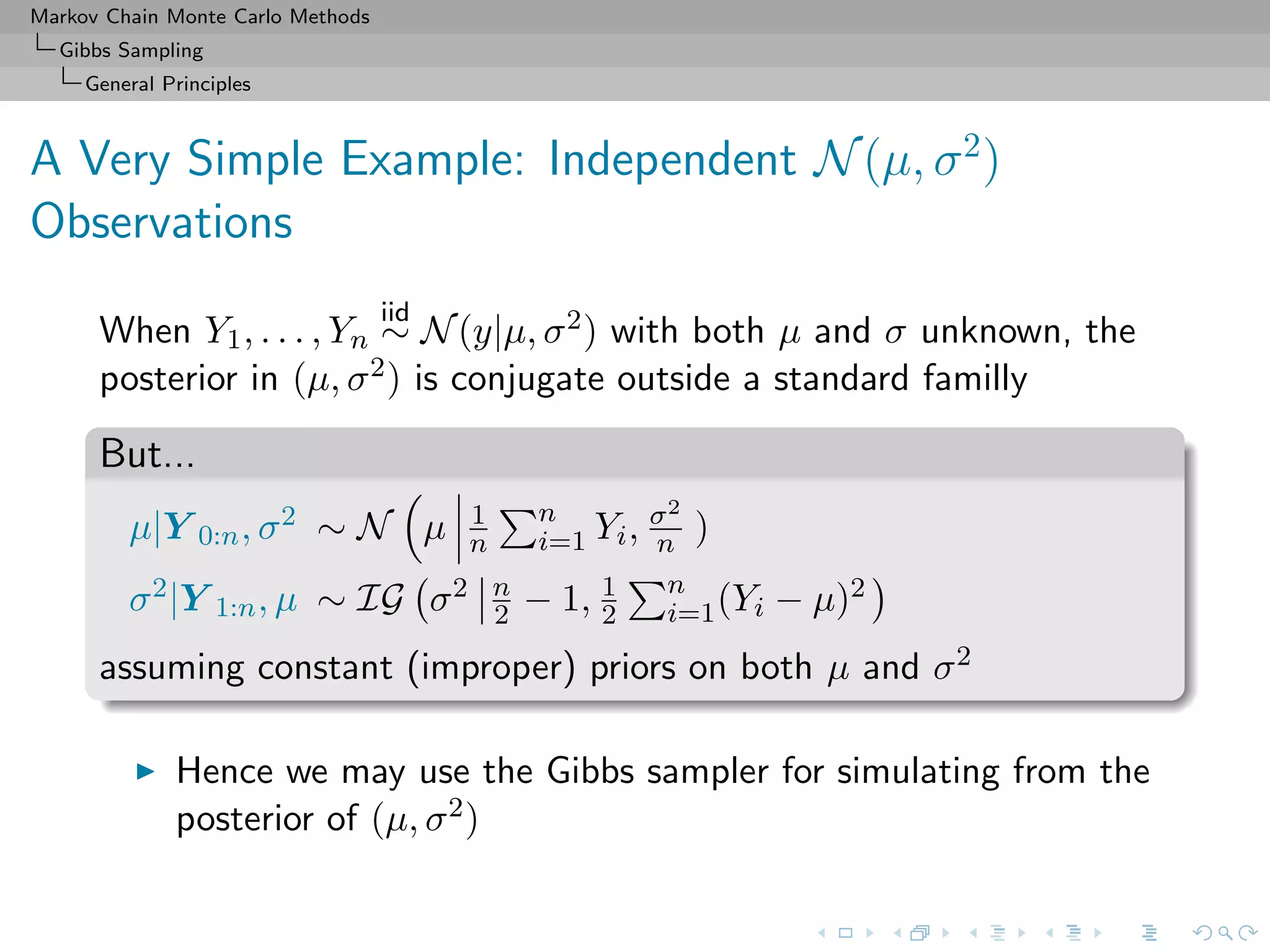
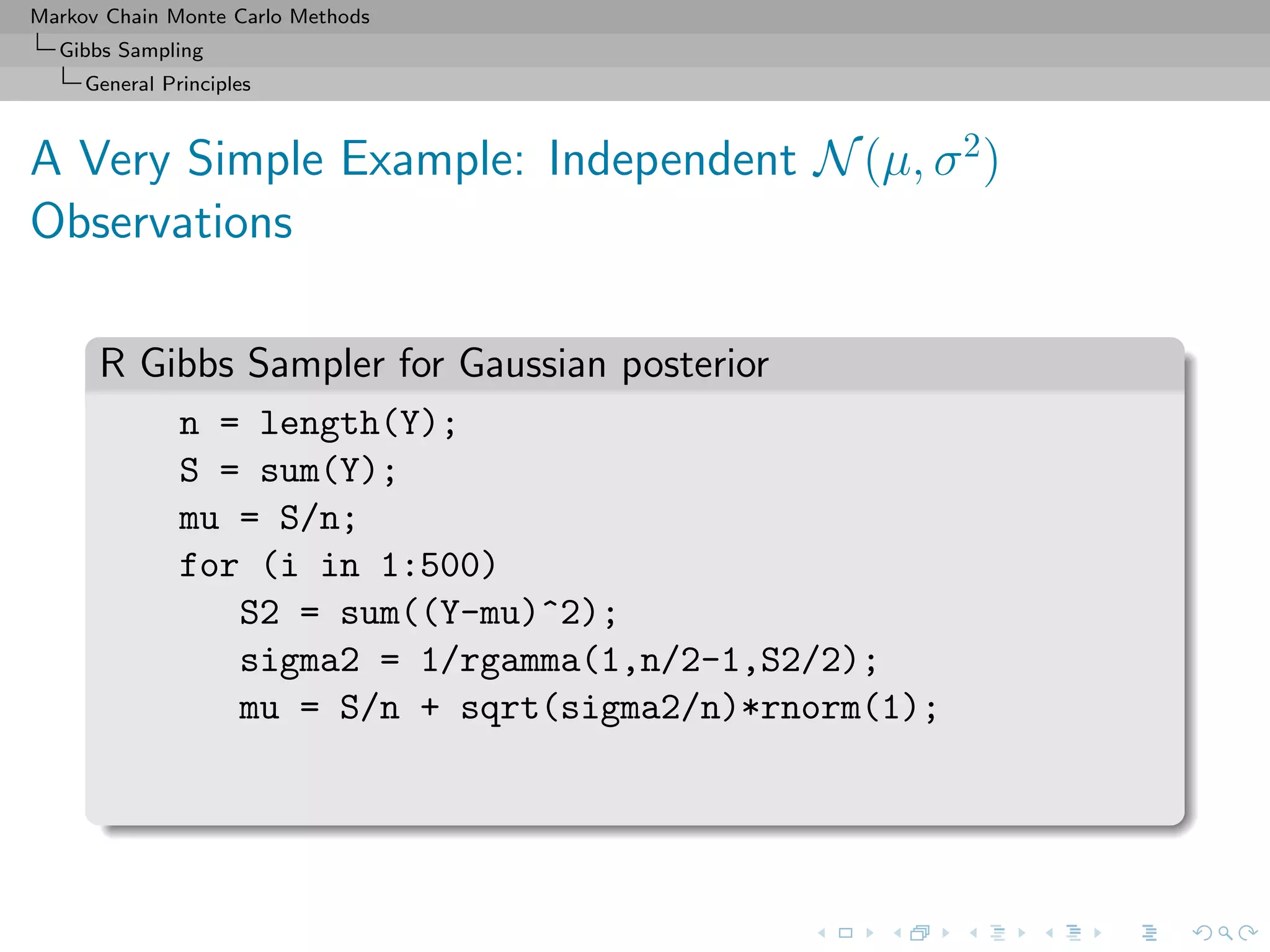
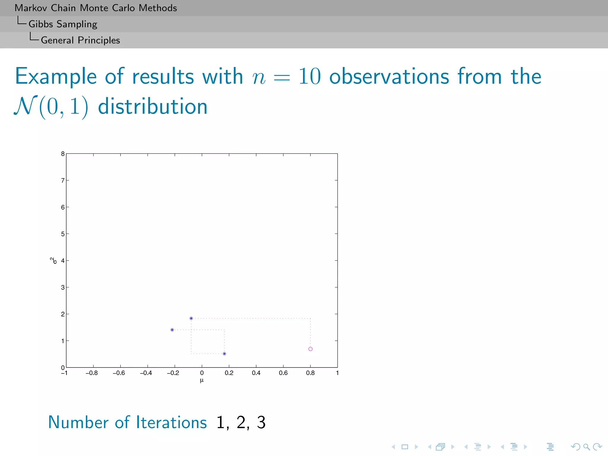
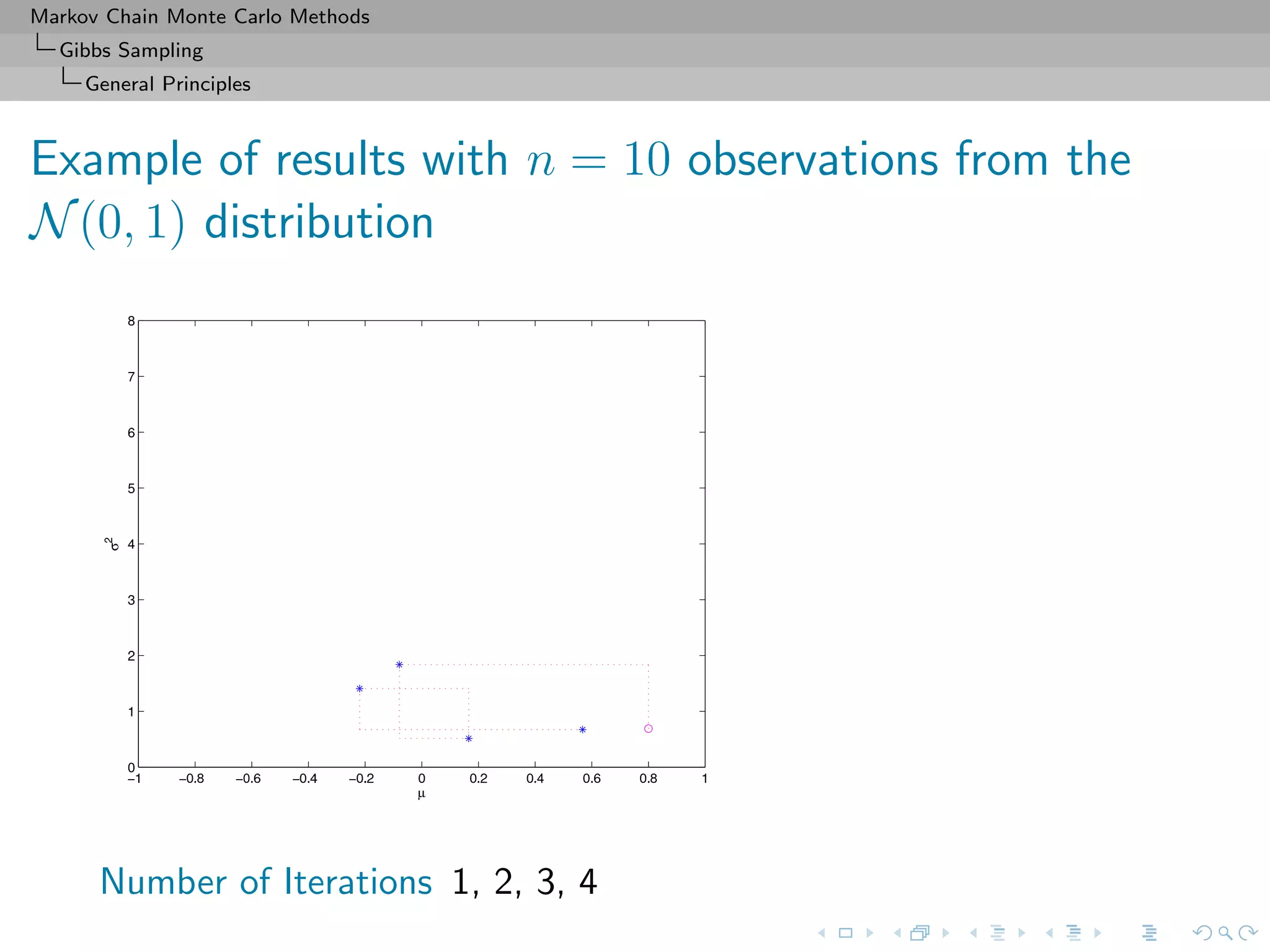

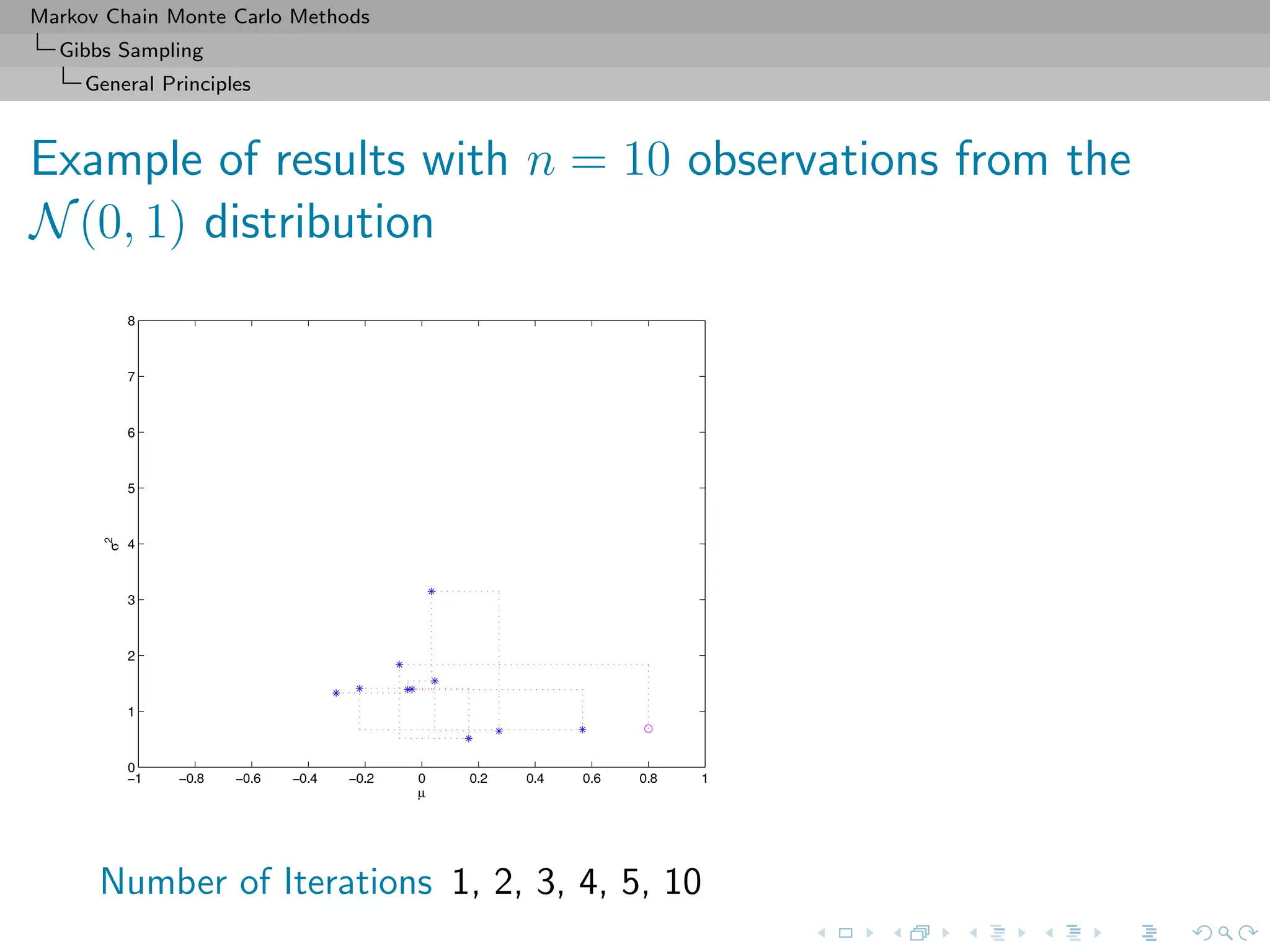
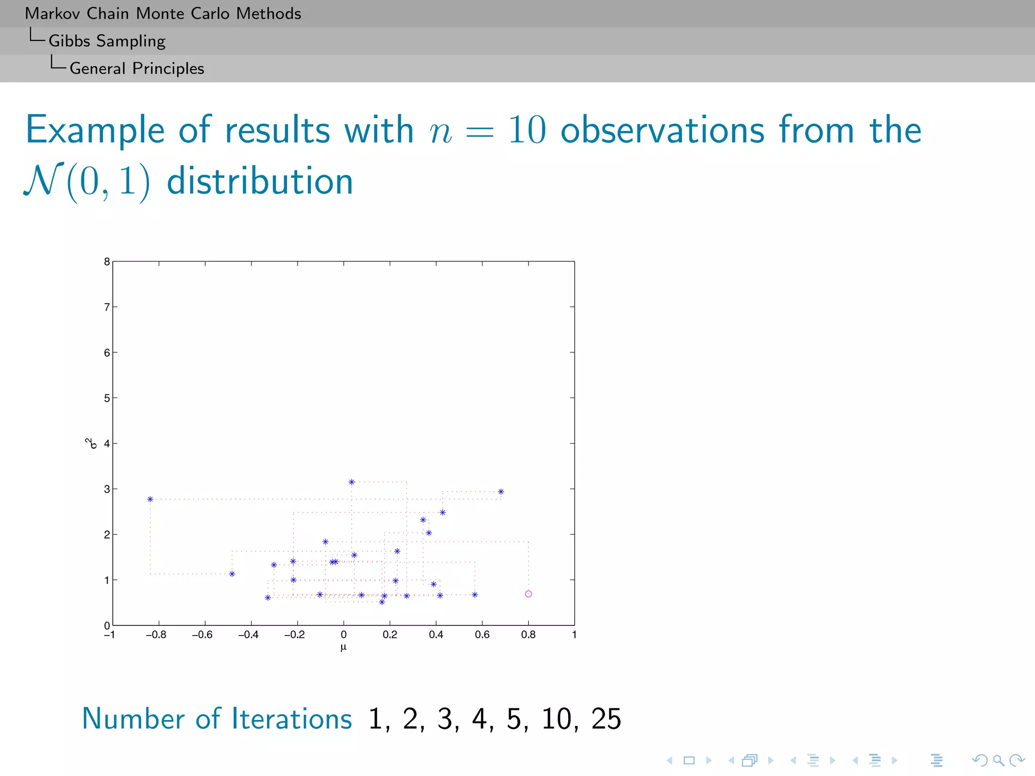
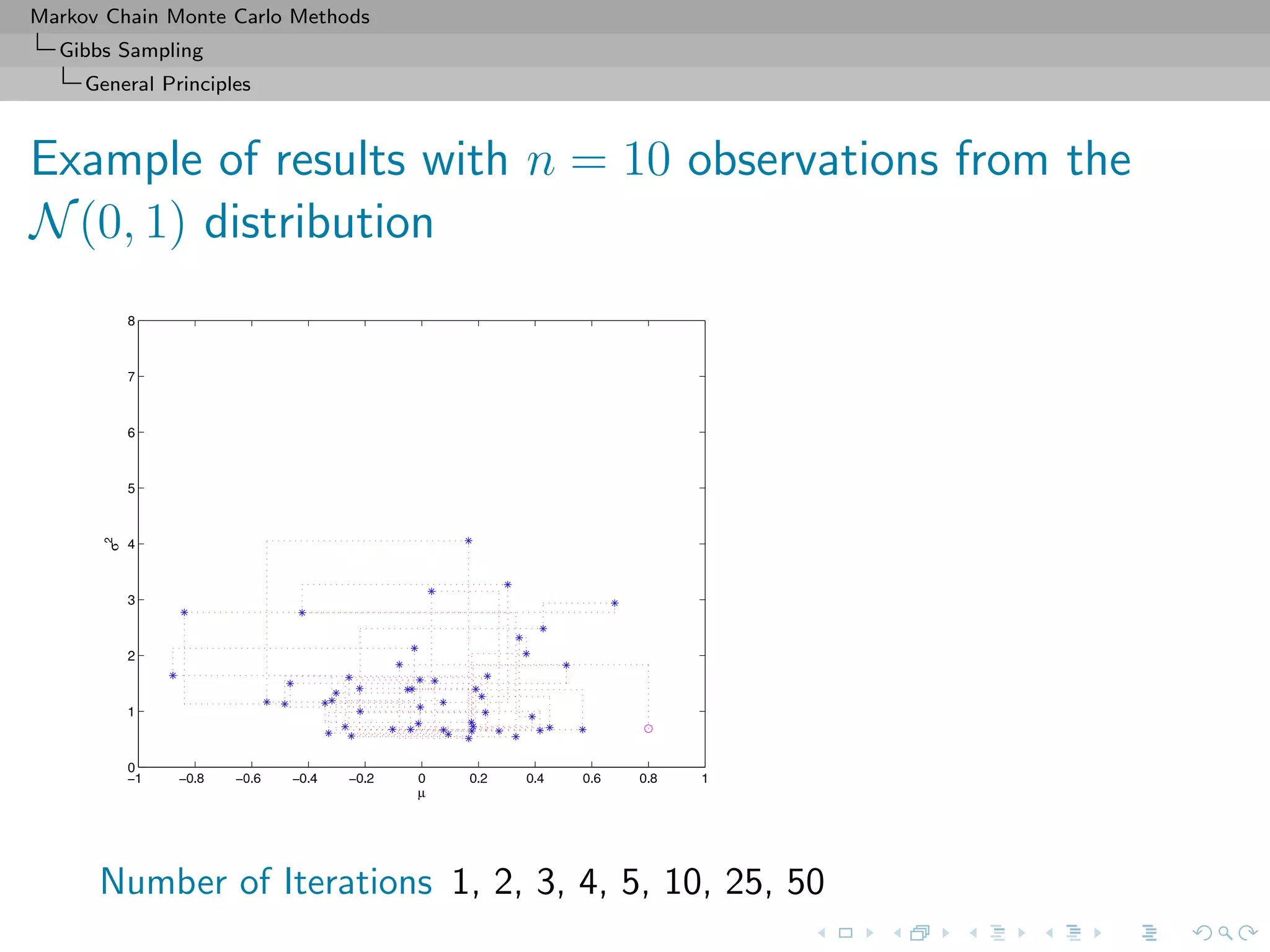
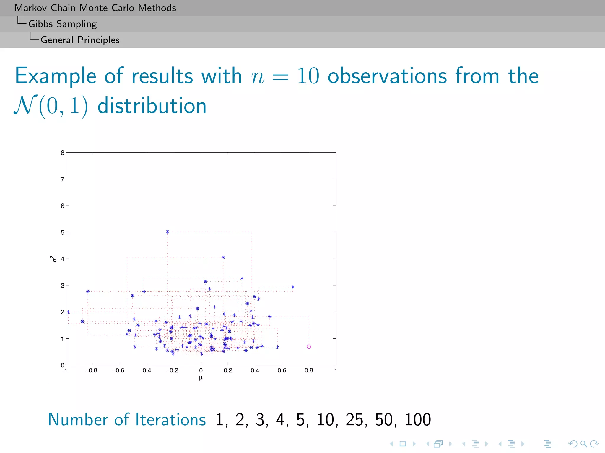
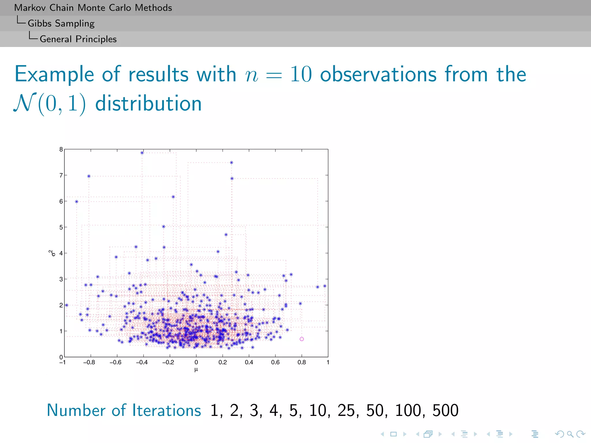
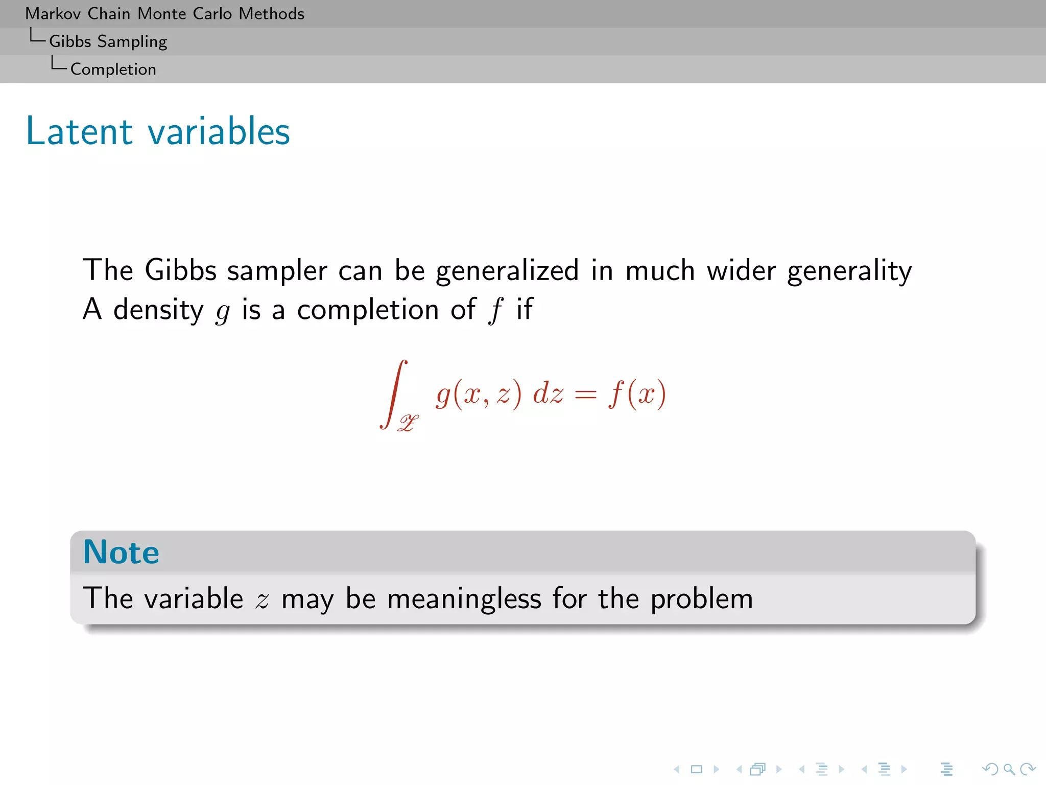


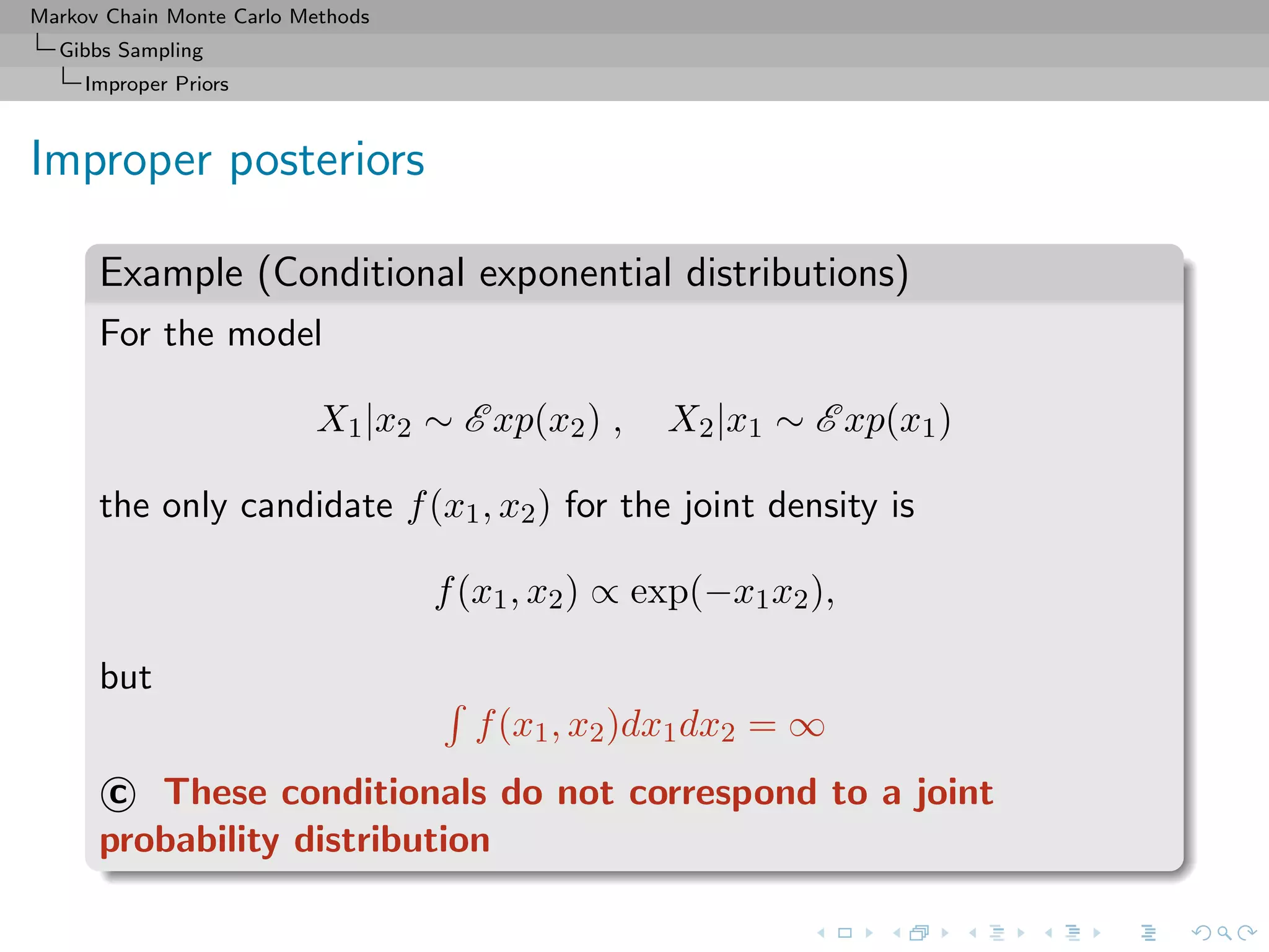
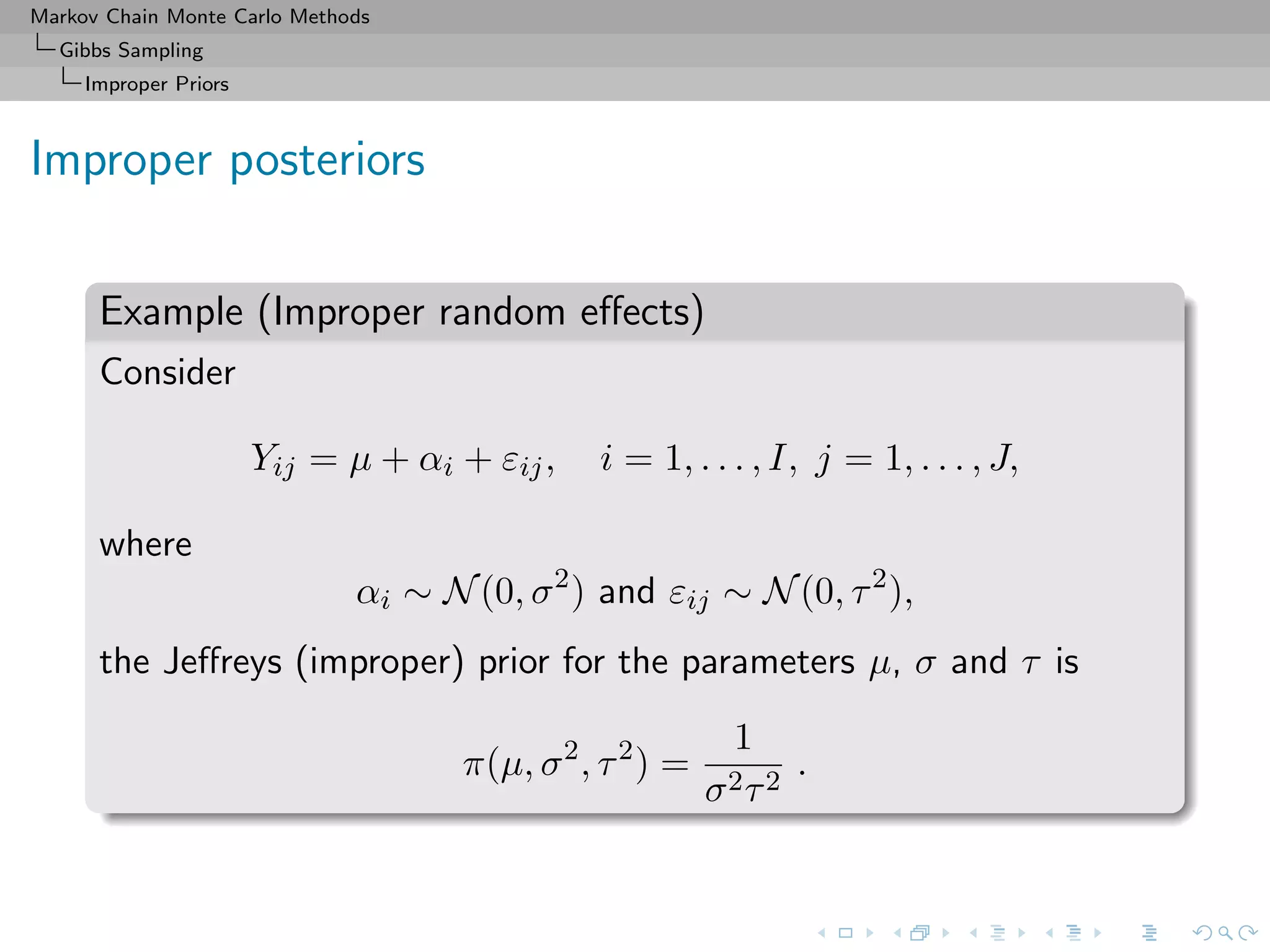
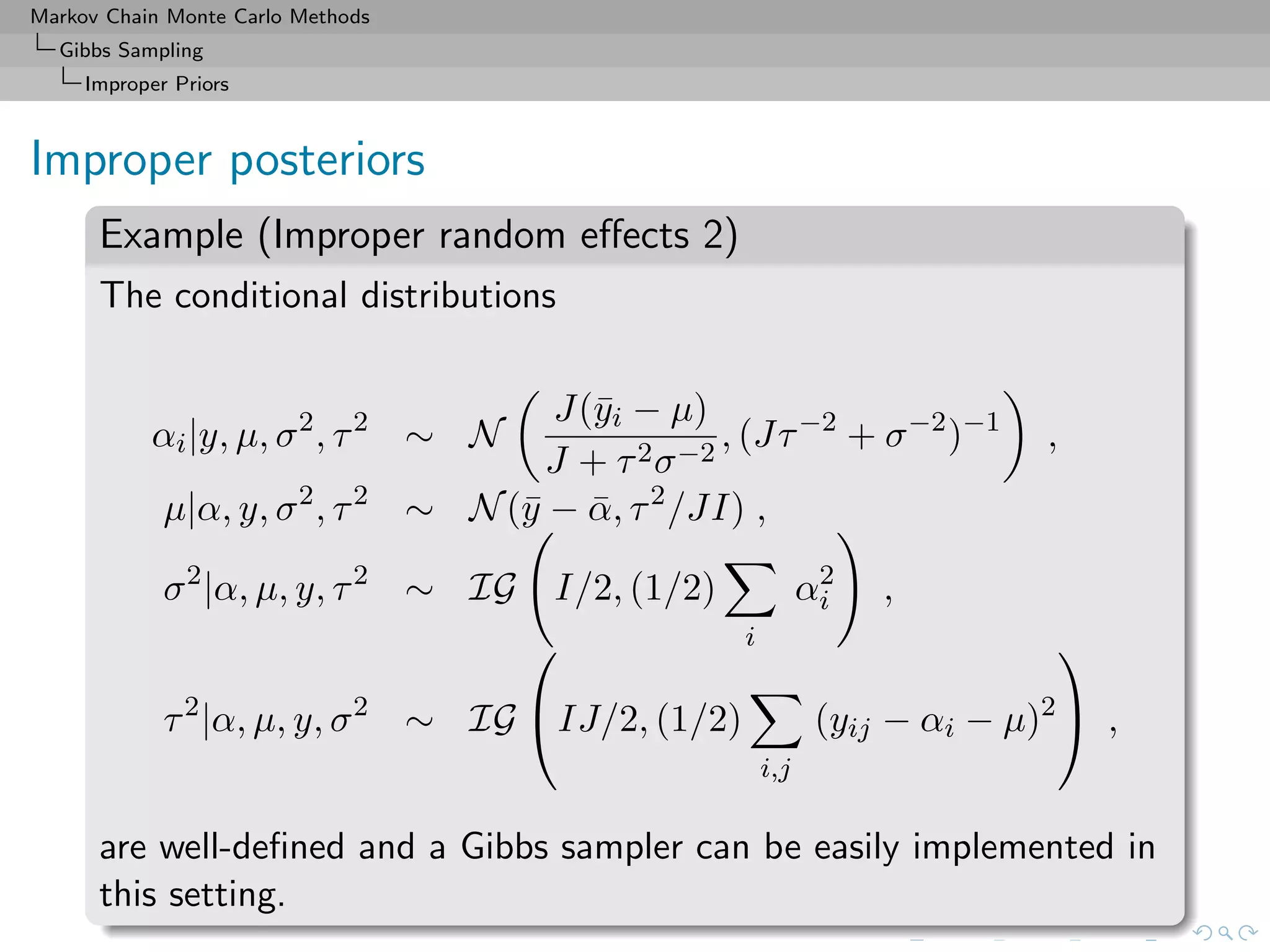
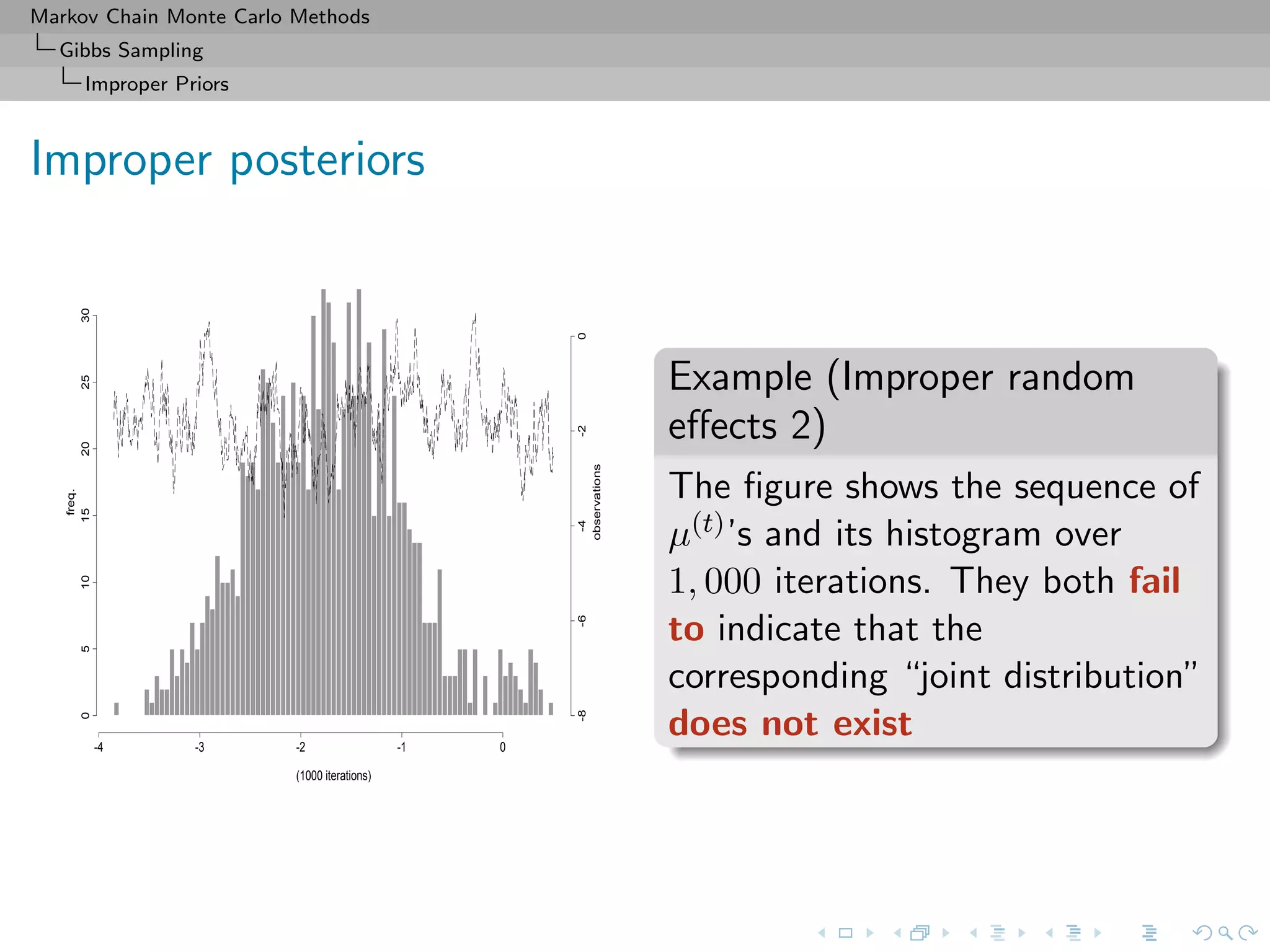
![Markov Chain Monte Carlo Methods
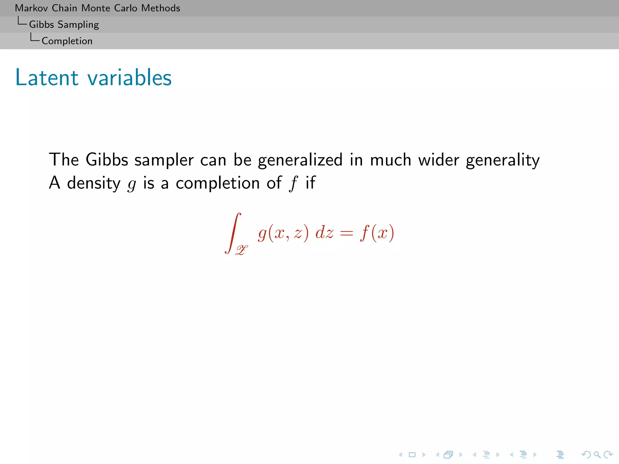
Gibbs Sampling
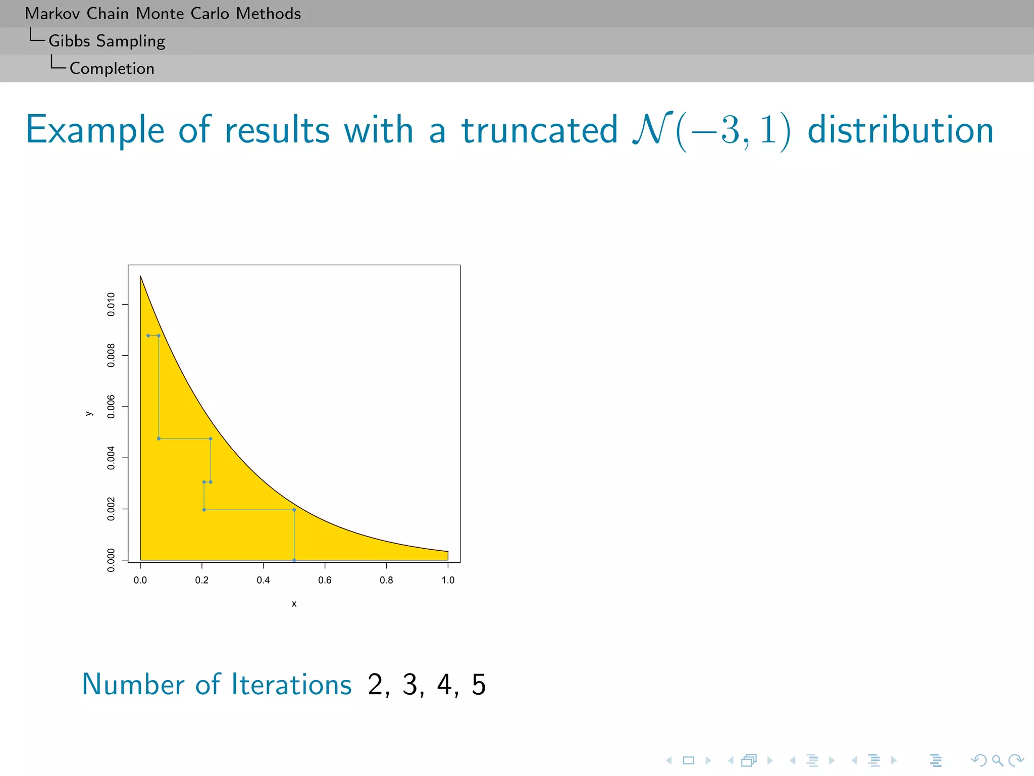
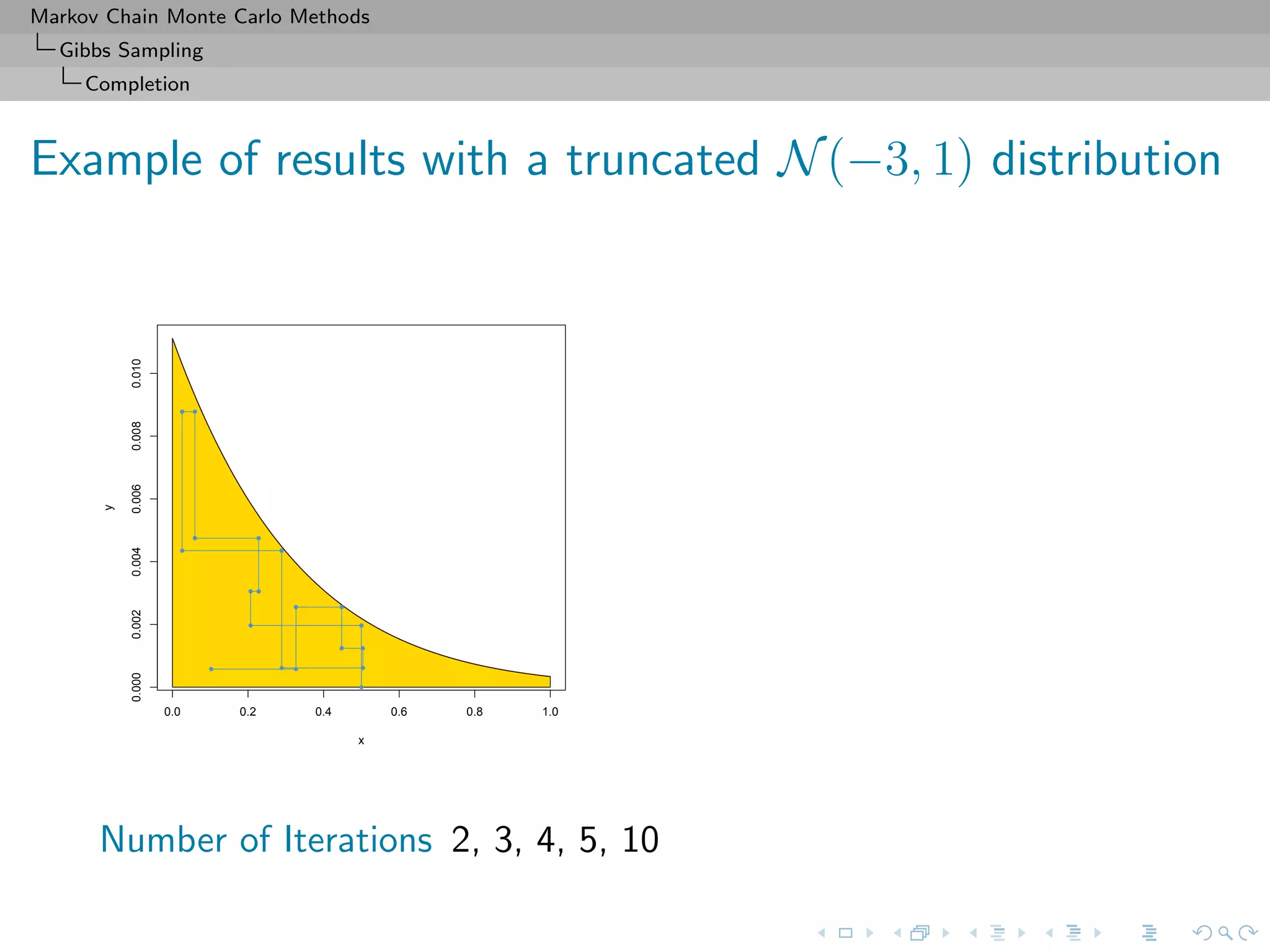
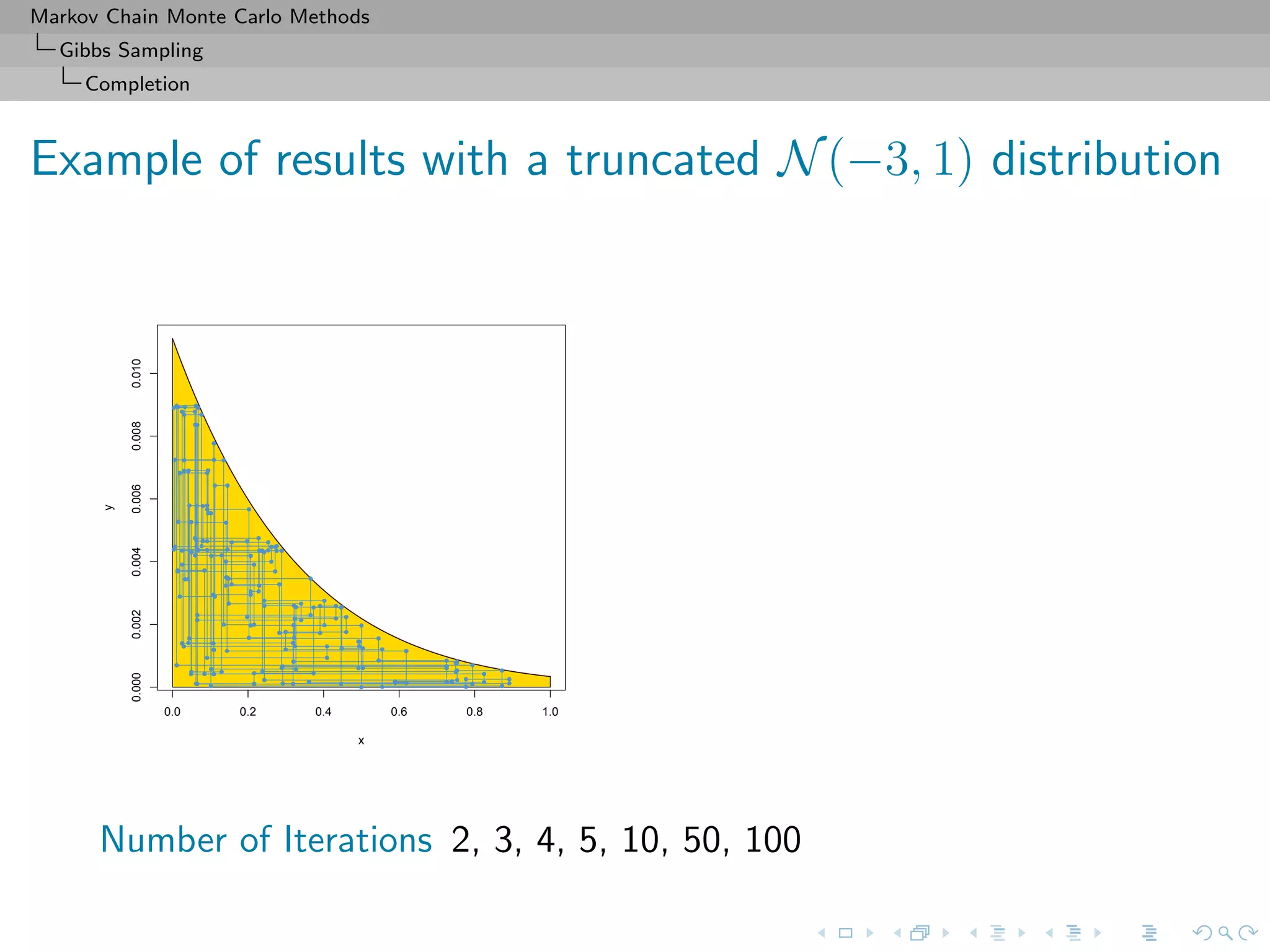
Completion
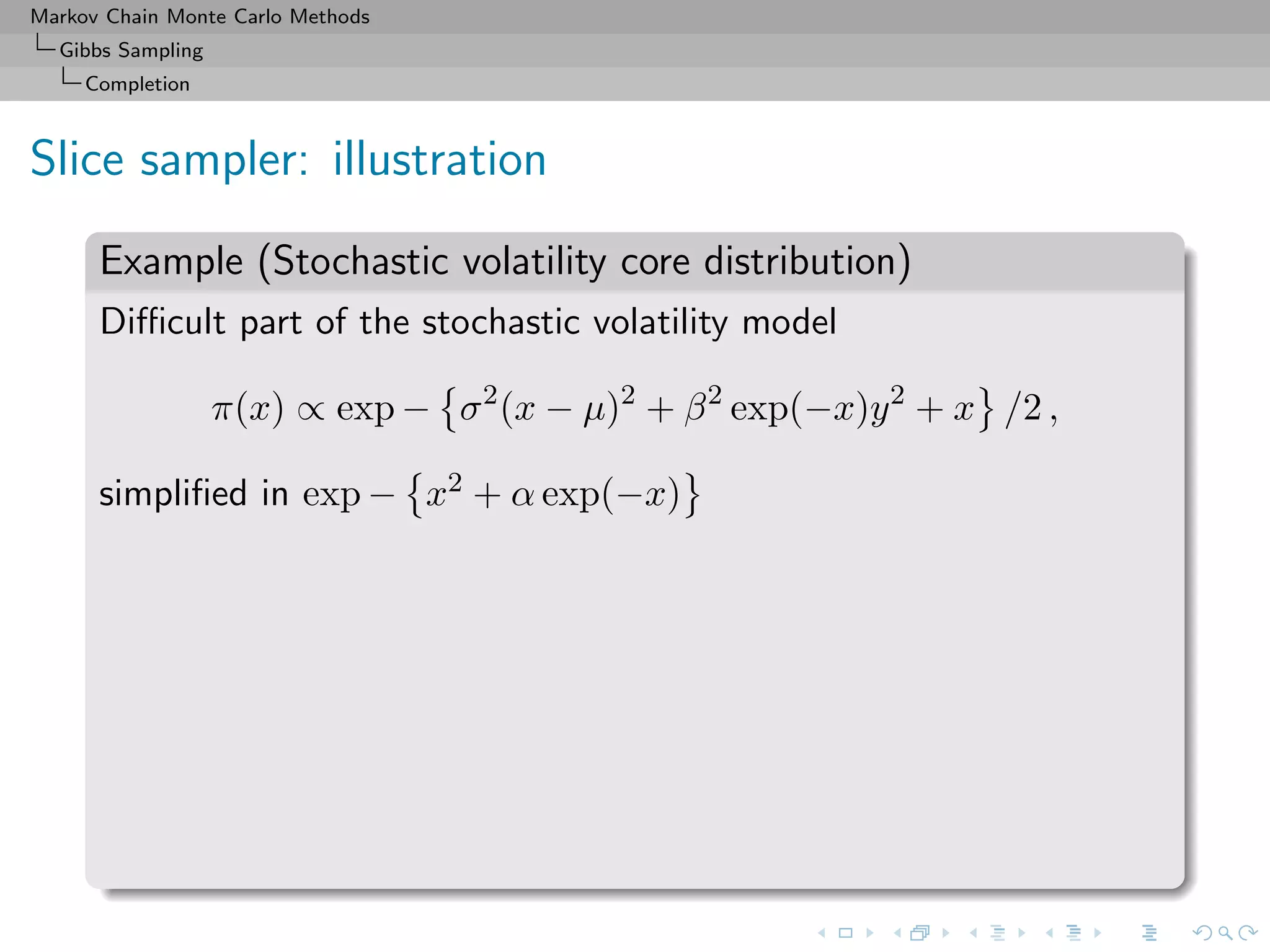
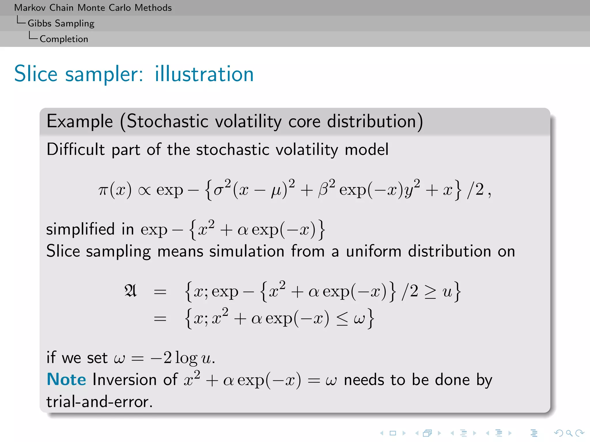
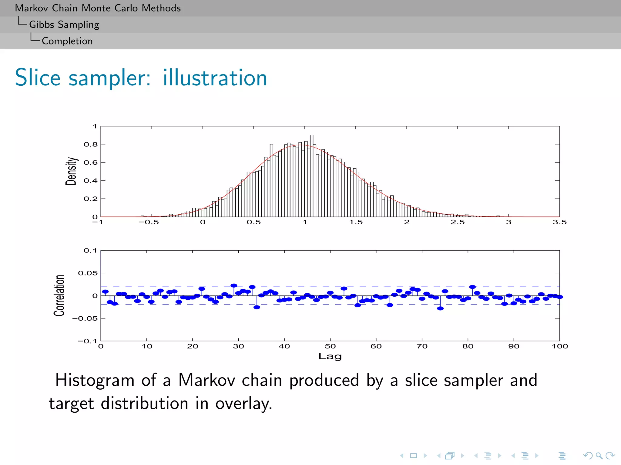
Slice sampler
Algorithm (Slice sampler)
Simulate
1. ω
(t+1)
1 ∼ U[0,f1(θ(t))];
. . .
k. ω
(t+1)
k ∼ U[0,fk(θ(t))];
k+1. θ(t+1) ∼ UA(t+1) , with
A(t+1)
= {y; fi(y) ≥ ω
(t+1)
i , i = 1, . . . , k}.](https://image.slidesharecdn.com/cirm-181022142714/75/short-course-at-CIRM-Bayesian-Masterclass-October-2018-113-2048.jpg)


![Markov Chain Monte Carlo Methods
Gibbs Sampling
Convergence
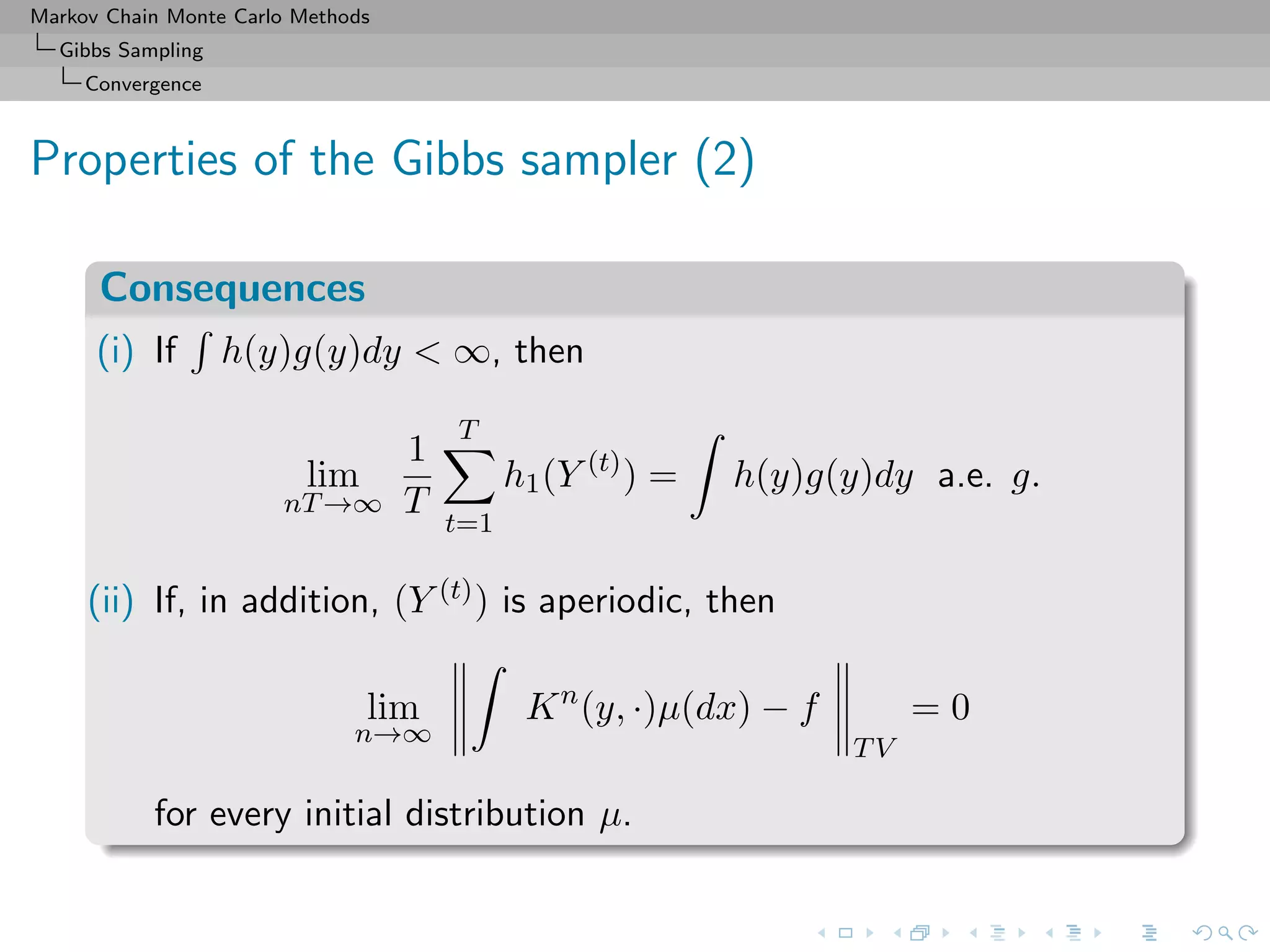
Properties of the Gibbs sampler
Theorem (Convergence)
For
(Y1, Y2, · · · , Yp) ∼ g(y1, . . . , yp),
if either
[Positivity condition]
(i) g(i)(yi) > 0 for every i = 1, · · · , p, implies that
g(y1, . . . , yp) > 0, where g(i) denotes the marginal distribution
of Yi, or
(ii) the transition kernel is absolutely continuous with respect to g,
then the chain is irreducible and positive Harris recurrent.](https://image.slidesharecdn.com/cirm-181022142714/75/short-course-at-CIRM-Bayesian-Masterclass-October-2018-125-2048.jpg)
![Markov Chain Monte Carlo Methods
Gibbs Sampling
Convergence
Slice sampler
fast on that slice
For convergence, the properties of Xt and of f(Xt) are identical
Theorem (Uniform ergodicity)
If f is bounded and suppf is bounded, the simple slice sampler is
uniformly ergodic.
[Mira & Tierney, 1997]](https://image.slidesharecdn.com/cirm-181022142714/75/short-course-at-CIRM-Bayesian-Masterclass-October-2018-127-2048.jpg)
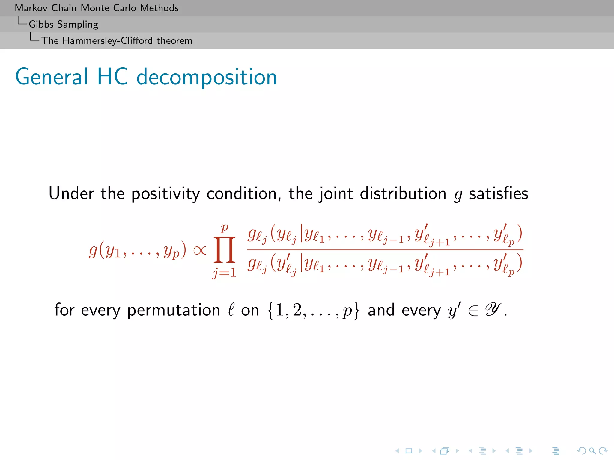
![Markov Chain Monte Carlo Methods
Gibbs Sampling
The Hammersley-Clifford theorem
Hammersley-Clifford theorem
An illustration that conditionals determine the joint distribution
Theorem
If the joint density g(y1, y2) have conditional distributions
g1(y1|y2) and g2(y2|y1), then
g(y1, y2) =
g2(y2|y1)
g2(v|y1)/g1(y1|v) dv
.
[Hammersley & Clifford, circa 1970]](https://image.slidesharecdn.com/cirm-181022142714/75/short-course-at-CIRM-Bayesian-Masterclass-October-2018-128-2048.jpg)
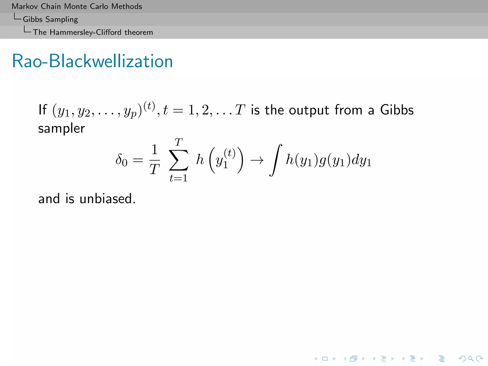
![Markov Chain Monte Carlo Methods
Gibbs Sampling
The Hammersley-Clifford theorem
Rao-Blackwellization (2)
Then
◦ Both estimators converge to I[h(Y1)]
◦ Both are unbiased,](https://image.slidesharecdn.com/cirm-181022142714/75/short-course-at-CIRM-Bayesian-Masterclass-October-2018-132-2048.jpg)
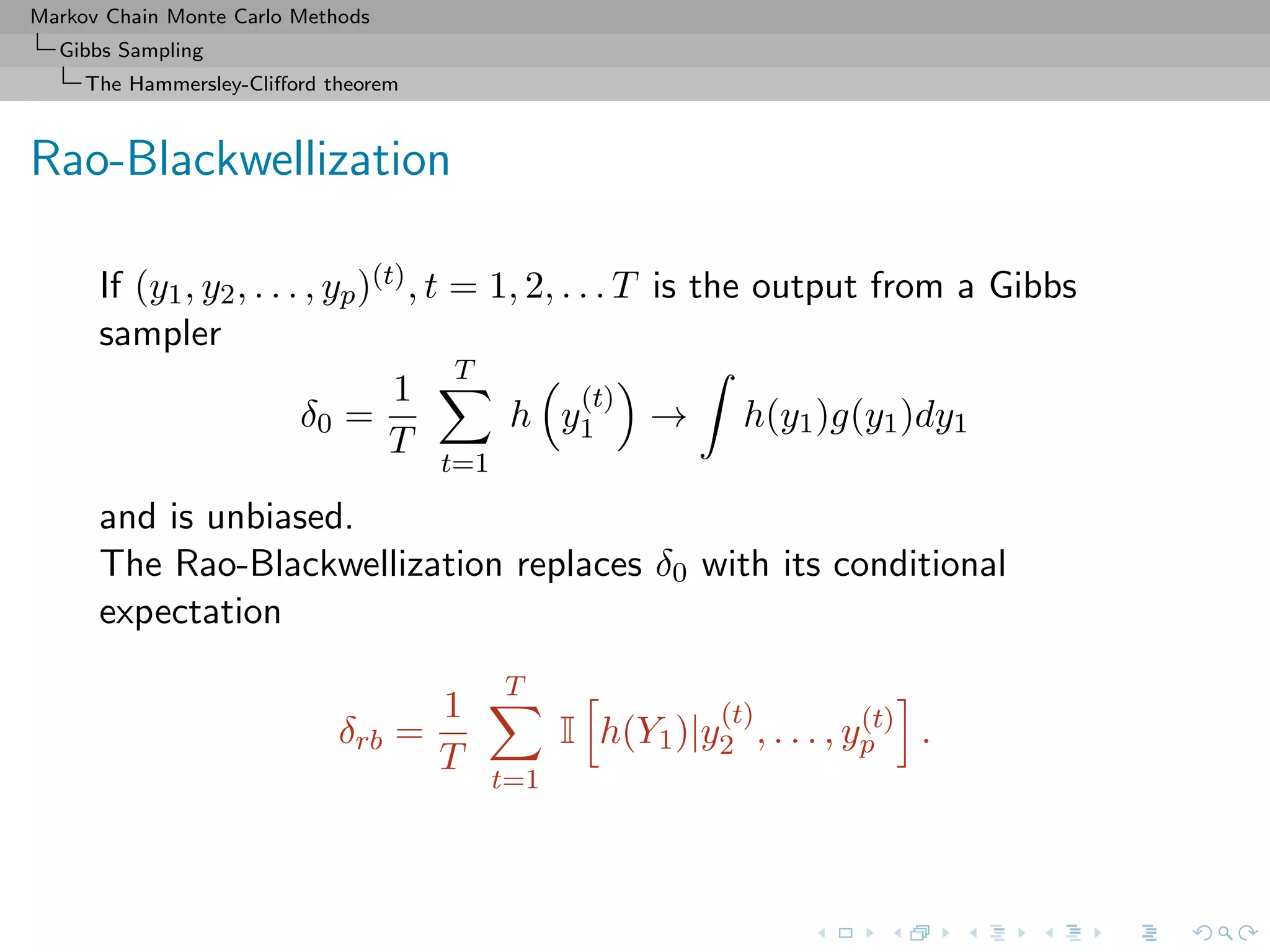
![Markov Chain Monte Carlo Methods
Gibbs Sampling
The Hammersley-Clifford theorem
Rao-Blackwellization (2)
Then
◦ Both estimators converge to I[h(Y1)]
◦ Both are unbiased,
◦ and
var I h(Y1)|Y
(t)
2 , . . . , Y (t)
p ≤ var(h(Y1)),
so δrb is uniformly better (for Data Augmentation)](https://image.slidesharecdn.com/cirm-181022142714/75/short-course-at-CIRM-Bayesian-Masterclass-October-2018-133-2048.jpg)
![Markov Chain Monte Carlo Methods
Gibbs Sampling
The Hammersley-Clifford theorem
Examples of Rao-Blackwellization
Example
Bivariate normal Gibbs sampler
X | y ∼ N(ρy, 1 − ρ2
)
Y | x ∼ N(ρx, 1 − ρ2
).
Then
δ0 =
1
T
T
i=1
X(i)
and δ1 =
1
T
T
i=1
I[X(i)
|Y (i)
] =
1
T
T
i=1
Y (i)
,
estimate I[X] and σ2
δ0
/σ2
δ1
= 1
ρ2 > 1.](https://image.slidesharecdn.com/cirm-181022142714/75/short-course-at-CIRM-Bayesian-Masterclass-October-2018-134-2048.jpg)
![Markov Chain Monte Carlo Methods
Gibbs Sampling
The Hammersley-Clifford theorem
Examples of Rao-Blackwellization (2)
Example (Poisson-Gamma Gibbs cont’d)
Na¨ıve estimate
δ0 =
1
T
T
t=1
λ(t)
and Rao-Blackwellized version
δπ
=
1
T
T
t=1
I[λ(t)
|x1, x2, . . . , x5, y
(i)
1 , y
(i)
2 , . . . , y
(i)
13 ]
=
1
360T
T
t=1
313 +
13
i=1
y
(t)
i ,
back to graph](https://image.slidesharecdn.com/cirm-181022142714/75/short-course-at-CIRM-Bayesian-Masterclass-October-2018-135-2048.jpg)


![Markov Chain Monte Carlo Methods
Hamiltonian Monte Carlo
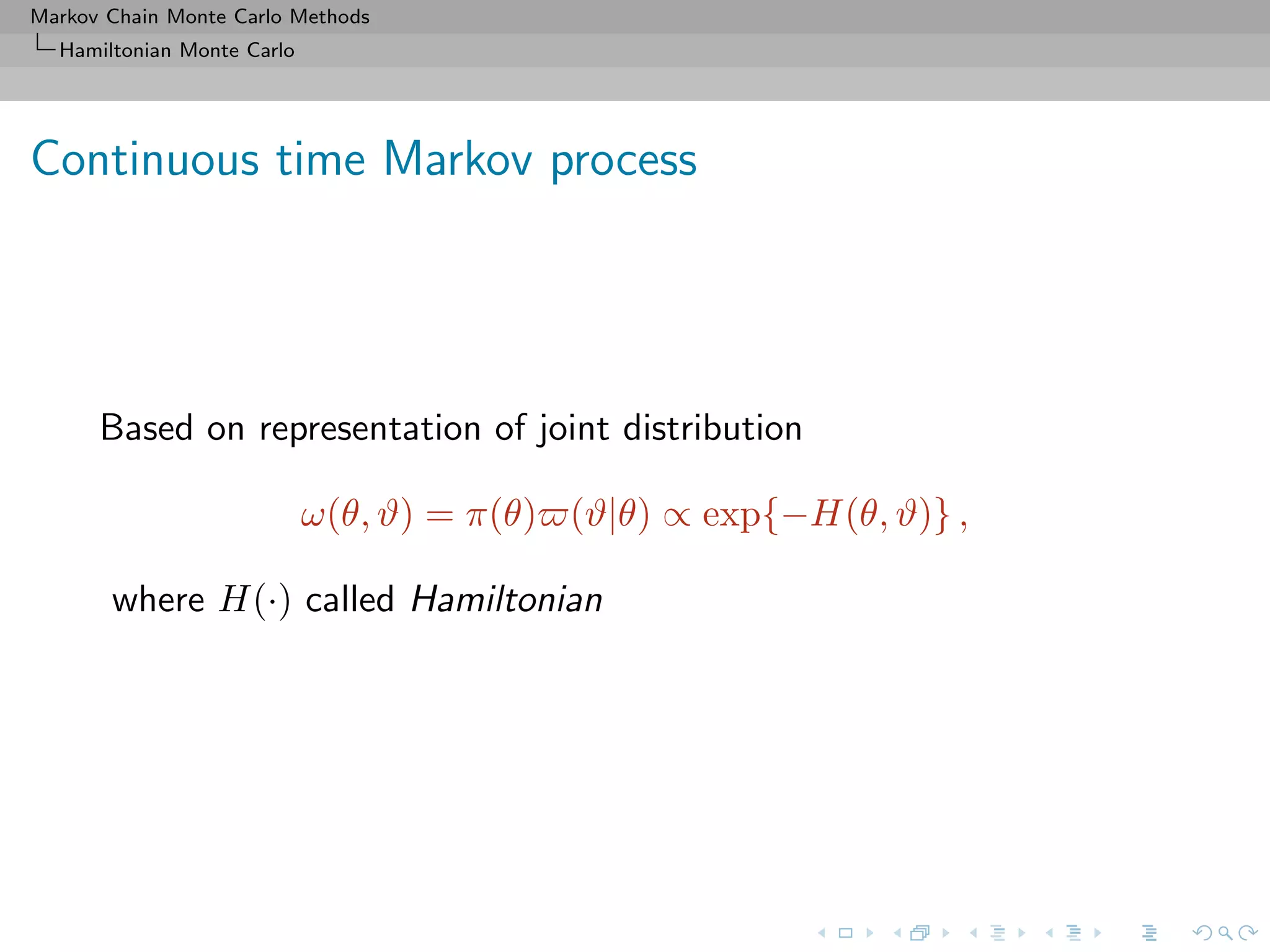
Background
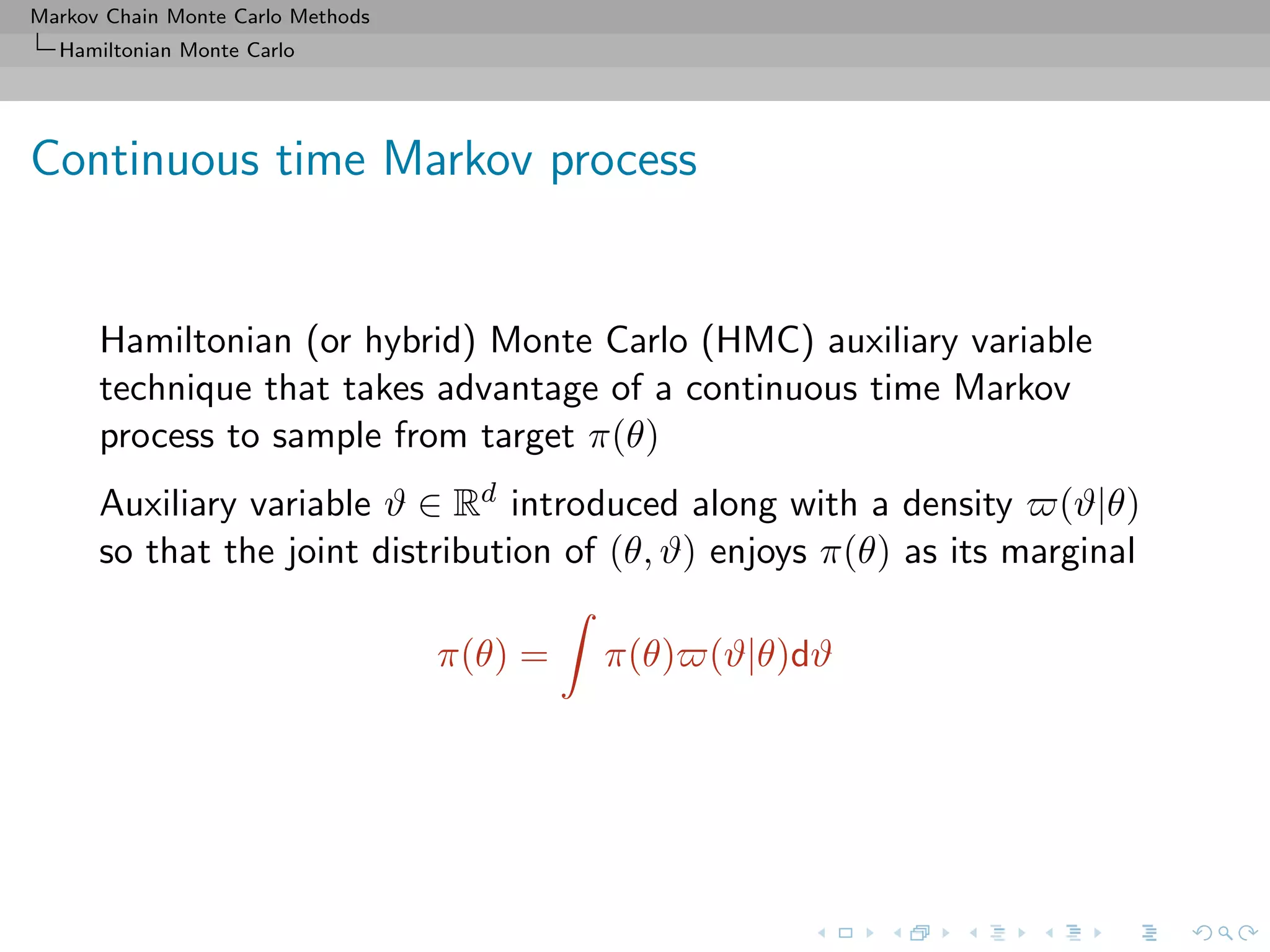
Approach from physics (Duane et al., 1987) popularised in
statistics by Neal (1996, 2002)
[Lan et al., 2016]](https://image.slidesharecdn.com/cirm-181022142714/75/short-course-at-CIRM-Bayesian-Masterclass-October-2018-154-2048.jpg)


![Markov Chain Monte Carlo Methods
Hamiltonian Monte Carlo
no U turns
empirically successful and popular version of HMC:
“no-U-turn sampler” (NUTS) adapts value of based on
primal-dual averaging
and eliminates need to choose trajectory length T via a
recursive algorithm that builds a set of candidate proposals for
a number of forward and backward leapfrog steps, stopping
automatically when simulated path traces back
[Hoffman and Gelman, 2014]](https://image.slidesharecdn.com/cirm-181022142714/75/short-course-at-CIRM-Bayesian-Masterclass-October-2018-162-2048.jpg)
![Markov Chain Monte Carlo Methods
Piecewise Deterministic Versions
Motivations
Motivation: piecewise deterministic Markov process
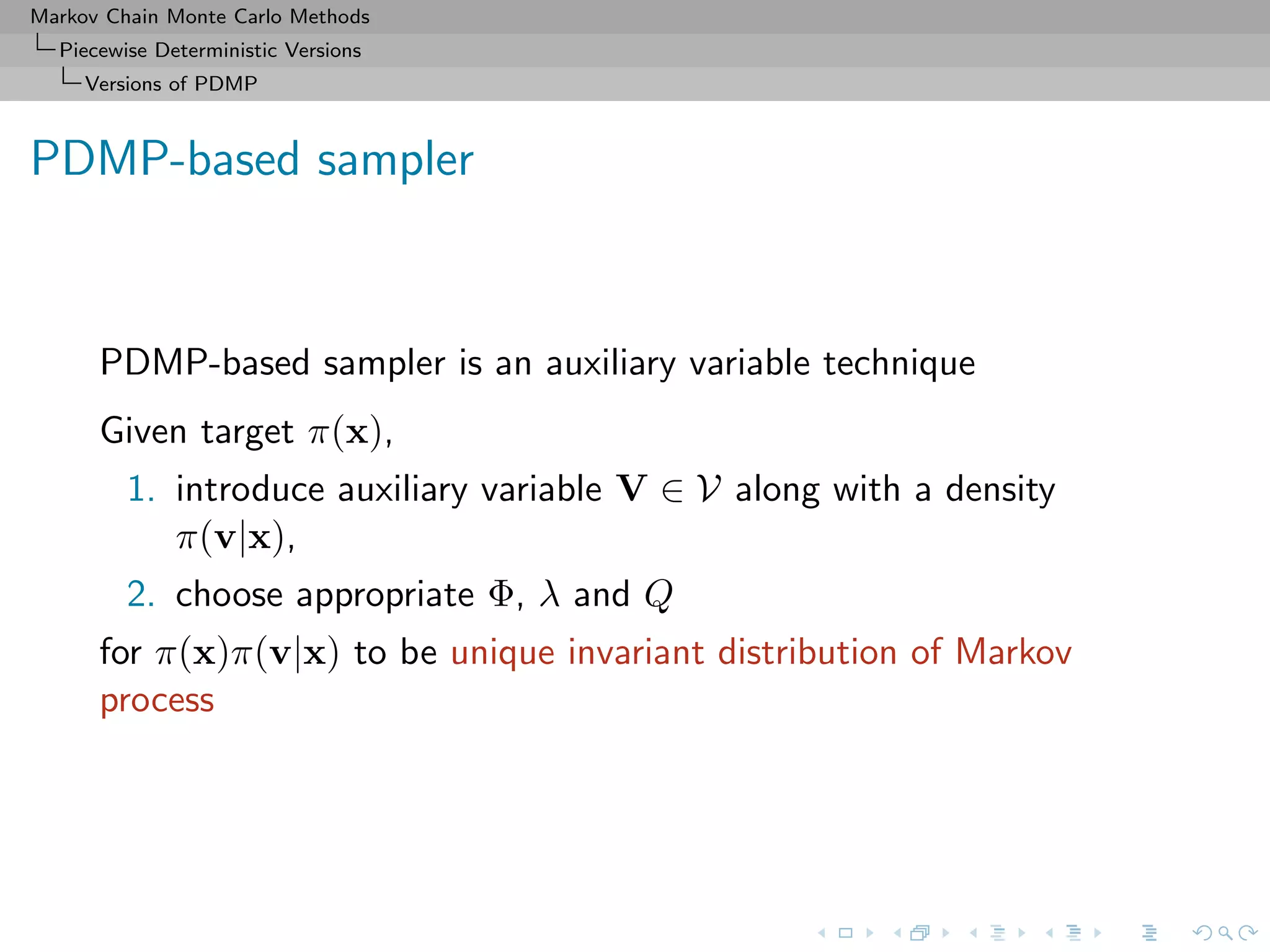
PDMP sampler is a (new?) continuous-time, non-reversible
MCMC method based on auxiliary variables
1. particle physics simulation
[Peters et al., 2012]
2. empirically state-of-the-art performances
[Bouchard et al., 2017]
3. exact subsampled in big data
[Bierkens et al., 2017]
4. geometric ergodicity for a large class of distribution
[Deligiannidis et al., 2017, Bierkens et al., 2017]
5. Ability to deal with intractable potential U(x) = Uω(x)µ(dω)
[Pakman et al., 2016]](https://image.slidesharecdn.com/cirm-181022142714/75/short-course-at-CIRM-Bayesian-Masterclass-October-2018-167-2048.jpg)
![Markov Chain Monte Carlo Methods
Piecewise Deterministic Versions
Motivations
Older versions
Use of alternative methodology based on Birth–&-Death (point)
process
Idea: Create Markov chain in continuous time, i.e. a Markov jump
process
Time till next modification (jump) exponentially distributed with
intensity q(θ, θ ) depending on current and future states.
[Preston, 1976; Ripley, 1977; Geyer & Møller, 1994; Stevens, 1999]](https://image.slidesharecdn.com/cirm-181022142714/75/short-course-at-CIRM-Bayesian-Masterclass-October-2018-169-2048.jpg)
![Markov Chain Monte Carlo Methods
Piecewise Deterministic Versions
Motivations
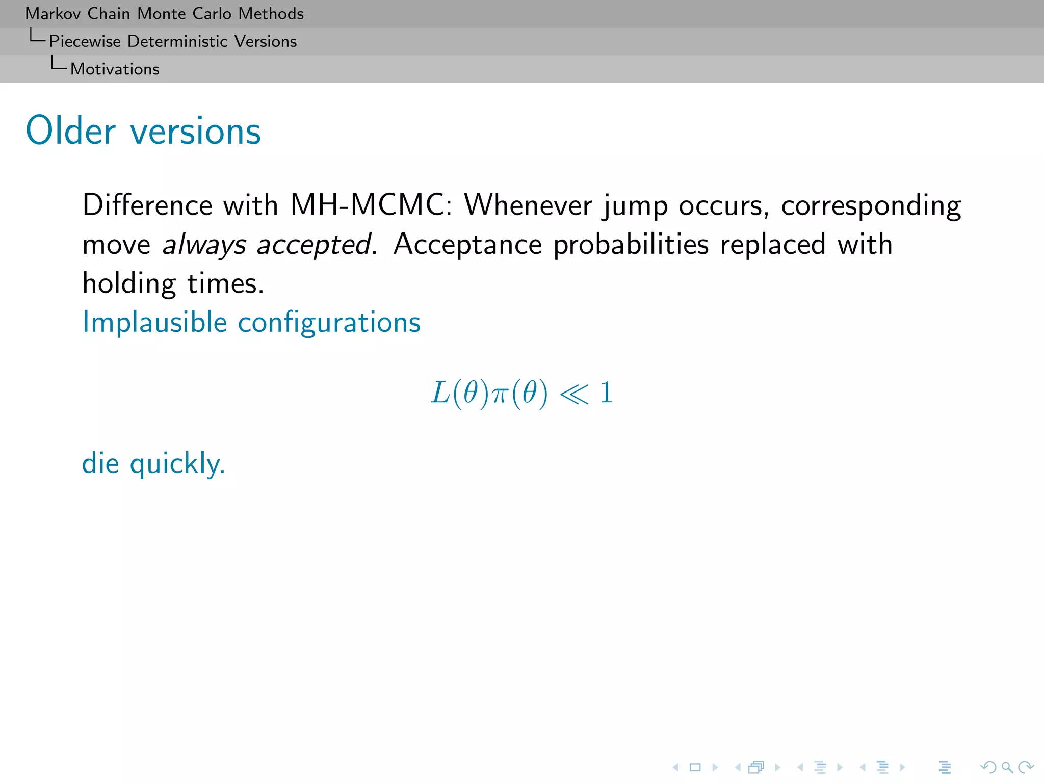
Older versions
Difference with MH-MCMC: Whenever jump occurs, corresponding
move always accepted. Acceptance probabilities replaced with
holding times.
Implausible configurations
L(θ)π(θ) 1
die quickly.
Sufficient to have detailed balance
L(θ)π(θ)q(θ, θ ) = L(θ )π(θ )q(θ , θ) for all θ, θ
for ˜π(θ) ∝ L(θ)π(θ) to be stationary.
[Capp´e et al., 2000]](https://image.slidesharecdn.com/cirm-181022142714/75/short-course-at-CIRM-Bayesian-Masterclass-October-2018-171-2048.jpg)
![Markov Chain Monte Carlo Methods
Piecewise Deterministic Versions
Motivations
Setup
All MCMC schemes presented here target an extended distribution
on Z = Rd × Rd
ρ(z) = π(x) × ψ(v) = exp(−H(z))
where z = (x, v) extended state and Ψ(v) [by default] multivariate
standard Normal
Physics takes v as velocity or momentum variables allowing for a
deterministic dynamics on Rd
Obviously sampling from ρ provides samples from π](https://image.slidesharecdn.com/cirm-181022142714/75/short-course-at-CIRM-Bayesian-Masterclass-October-2018-172-2048.jpg)
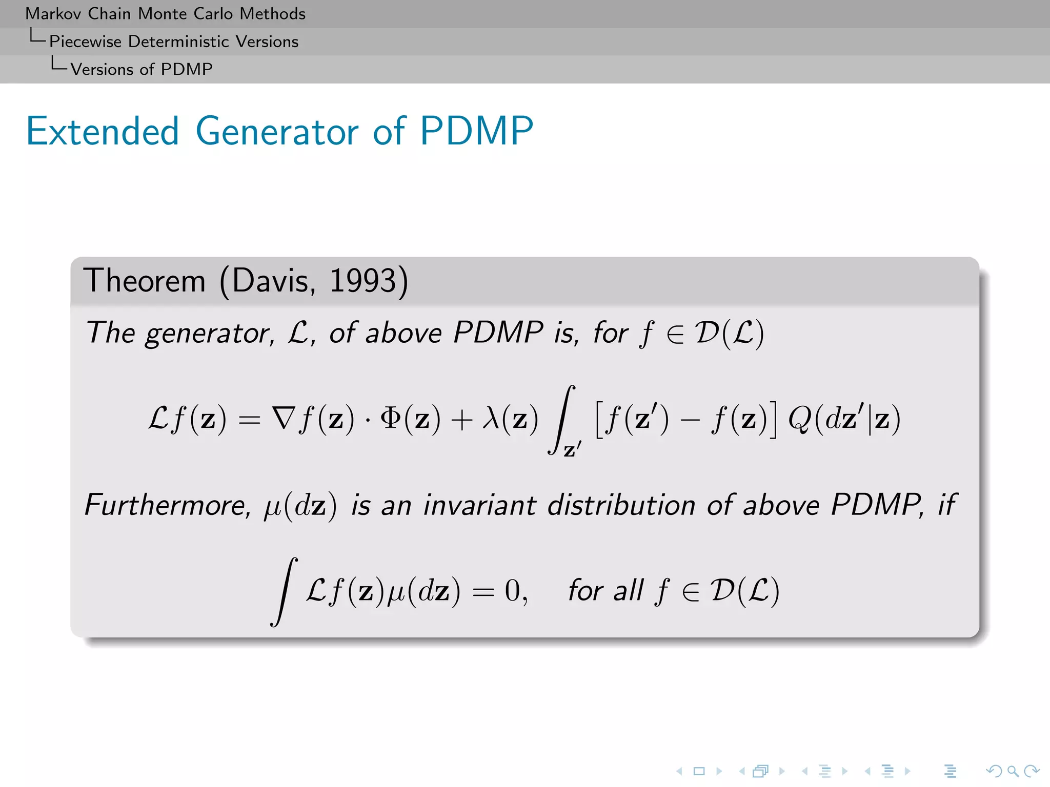
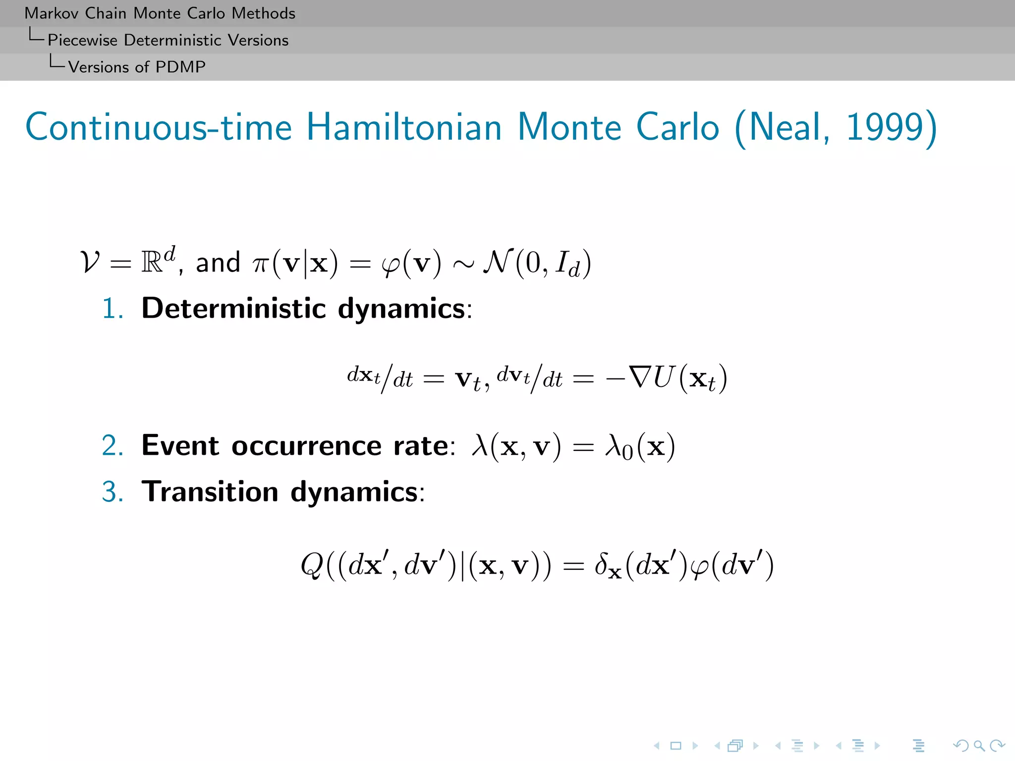
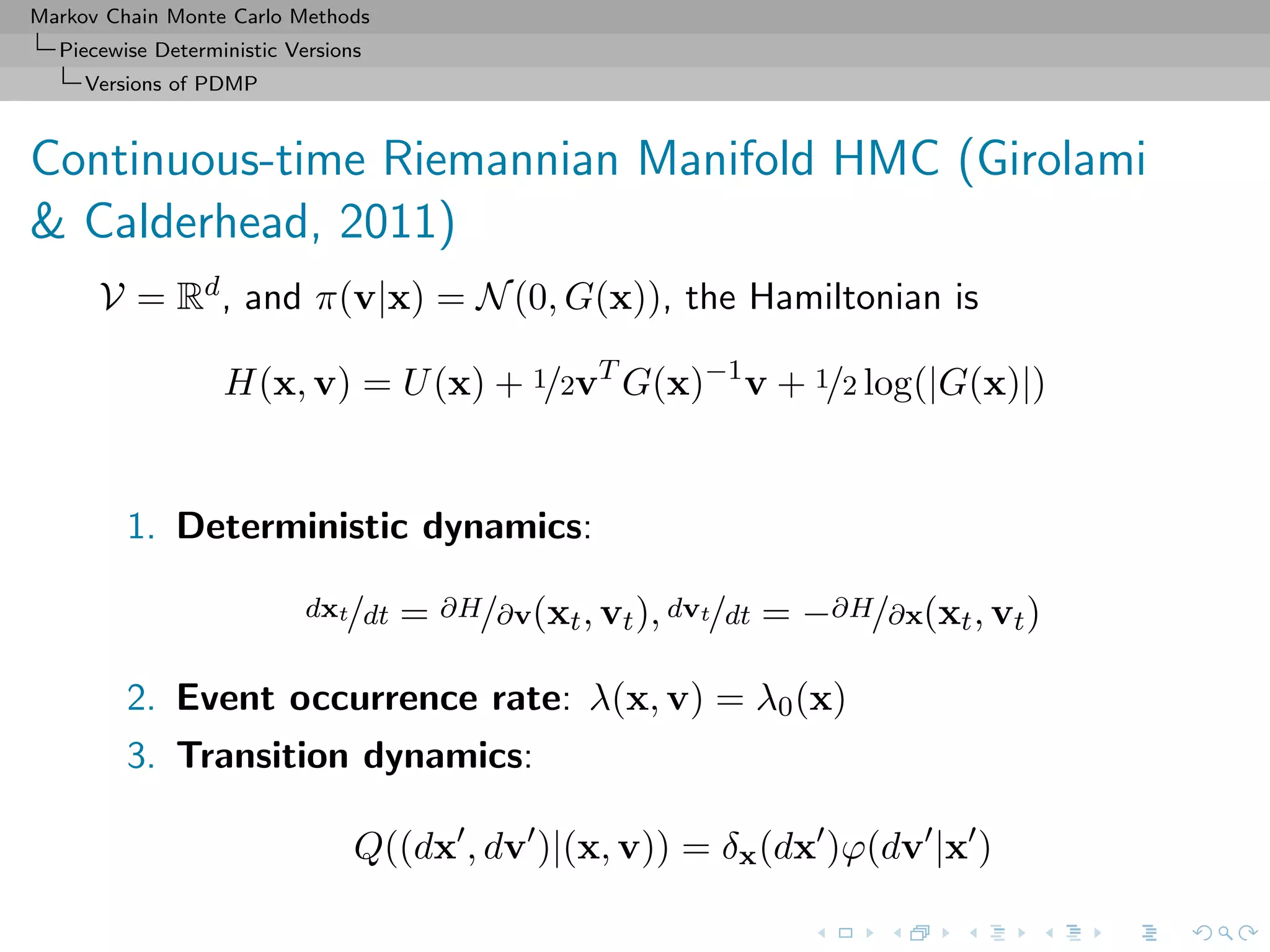
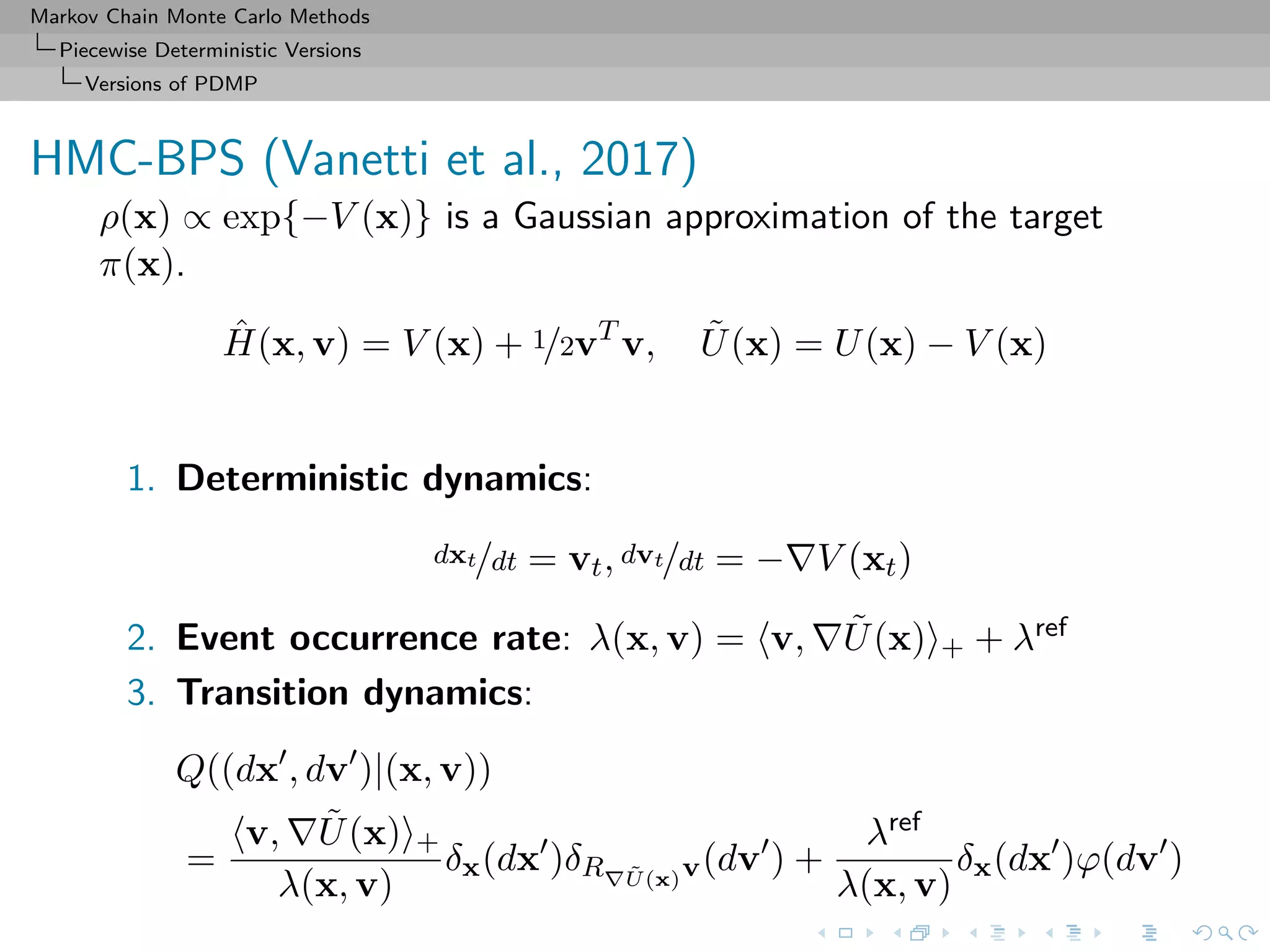
![Markov Chain Monte Carlo Methods
Piecewise Deterministic Versions
Motivations
Piecewise deterministic Markov process
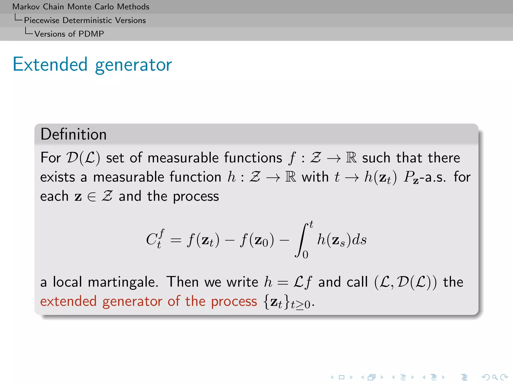
Piecewise deterministic Markov process {zt ∈ Z}t∈[0,∞), with
three ingredients,
1. Deterministic dynamics: between events, deterministic
evolution based on ODE
dzt/dt = Φ(zt)
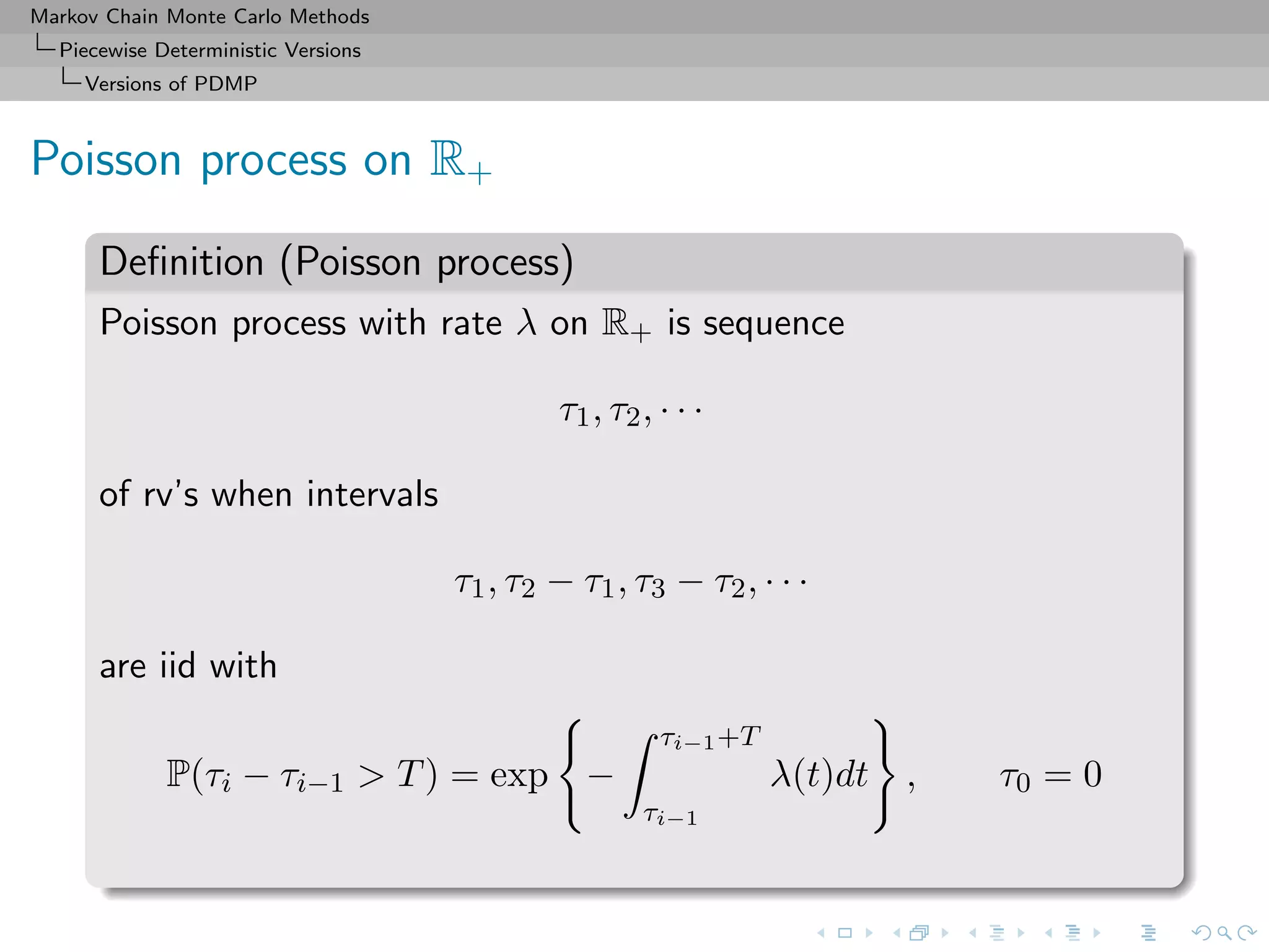
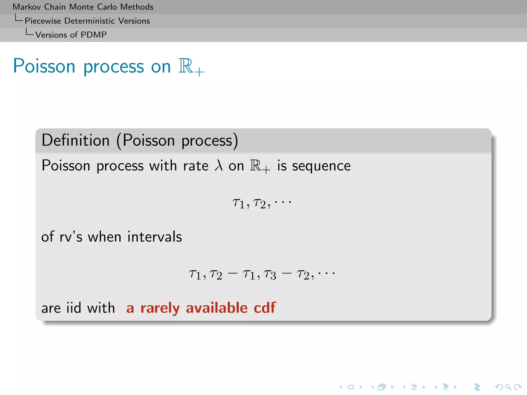
2. Event occurrence rate: λ(t) = λ(zt)
3. Transition dynamics: At event time, τ, state prior to τ
denoted by zτ−, and new state generated by zτ ∼ Q(·|zτ−).
[Davis, 1984, 1993]](https://image.slidesharecdn.com/cirm-181022142714/75/short-course-at-CIRM-Bayesian-Masterclass-October-2018-173-2048.jpg)
![Markov Chain Monte Carlo Methods
Piecewise Deterministic Versions
Versions of PDMP
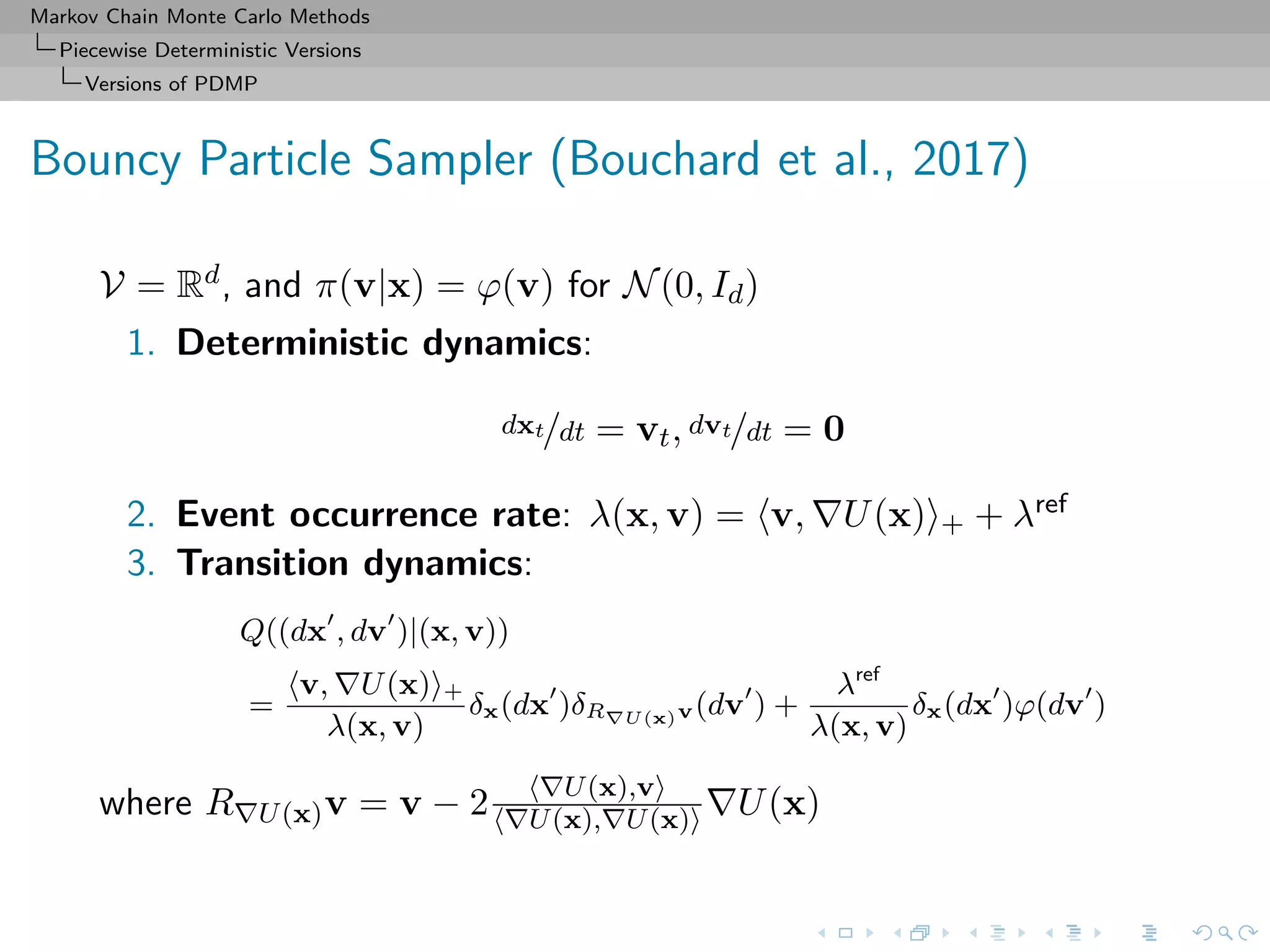
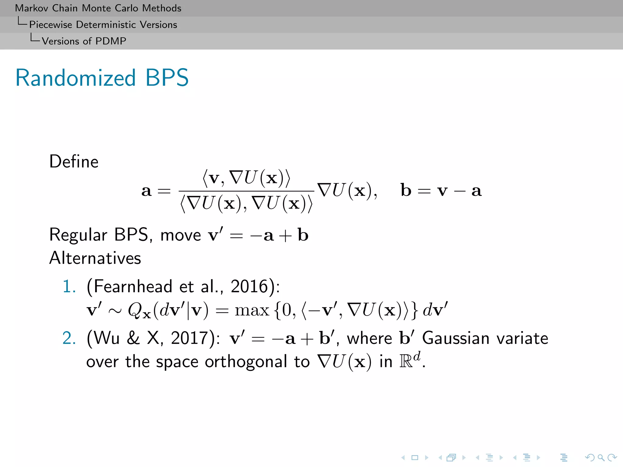
Basic bouncy particle sampler
Simulation of continuous-time piecewise linear trajectory (xt)t with
each segment in trajectory specified by
initial position x
length τ
velocity v
[Bouchard et al., 2017]](https://image.slidesharecdn.com/cirm-181022142714/75/short-course-at-CIRM-Bayesian-Masterclass-October-2018-176-2048.jpg)
![Markov Chain Monte Carlo Methods
Piecewise Deterministic Versions
Versions of PDMP
Basic bouncy particle sampler
Simulation of continuous-time piecewise linear trajectory (xt)t with
each segment in trajectory specified by
initial position x
length τ
velocity v
length specified by inhomogeneous Poisson point process with
intensity function
λ(x, v) = max{0, < U(x), v >}
[Bouchard et al., 2017]](https://image.slidesharecdn.com/cirm-181022142714/75/short-course-at-CIRM-Bayesian-Masterclass-October-2018-177-2048.jpg)
![Markov Chain Monte Carlo Methods
Piecewise Deterministic Versions
Versions of PDMP
Basic bouncy particle sampler
Simulation of continuous-time piecewise linear trajectory (xt)t with
each segment in trajectory specified by
initial position x
length τ
velocity v
new velocity after bouncing given by Newtonian elastic collision
R(x)v = v − 2
< U(x), v >
|| U(x)||2
U(x)
[Bouchard et al., 2017]](https://image.slidesharecdn.com/cirm-181022142714/75/short-course-at-CIRM-Bayesian-Masterclass-October-2018-178-2048.jpg)
![Markov Chain Monte Carlo Methods
Piecewise Deterministic Versions
Versions of PDMP
Basic bouncy particle sampler
[Bouchard et al., 2017]](https://image.slidesharecdn.com/cirm-181022142714/75/short-course-at-CIRM-Bayesian-Masterclass-October-2018-179-2048.jpg)
![Markov Chain Monte Carlo Methods
Piecewise Deterministic Versions
Versions of PDMP
Implementation hardships
Generally speaking, the main difficulties of implementing PDMP
come from
1. Computing the ODE flow Ψ: linear dynamic, quadratic
dynamic
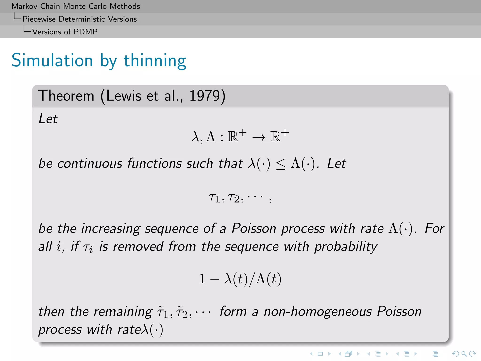
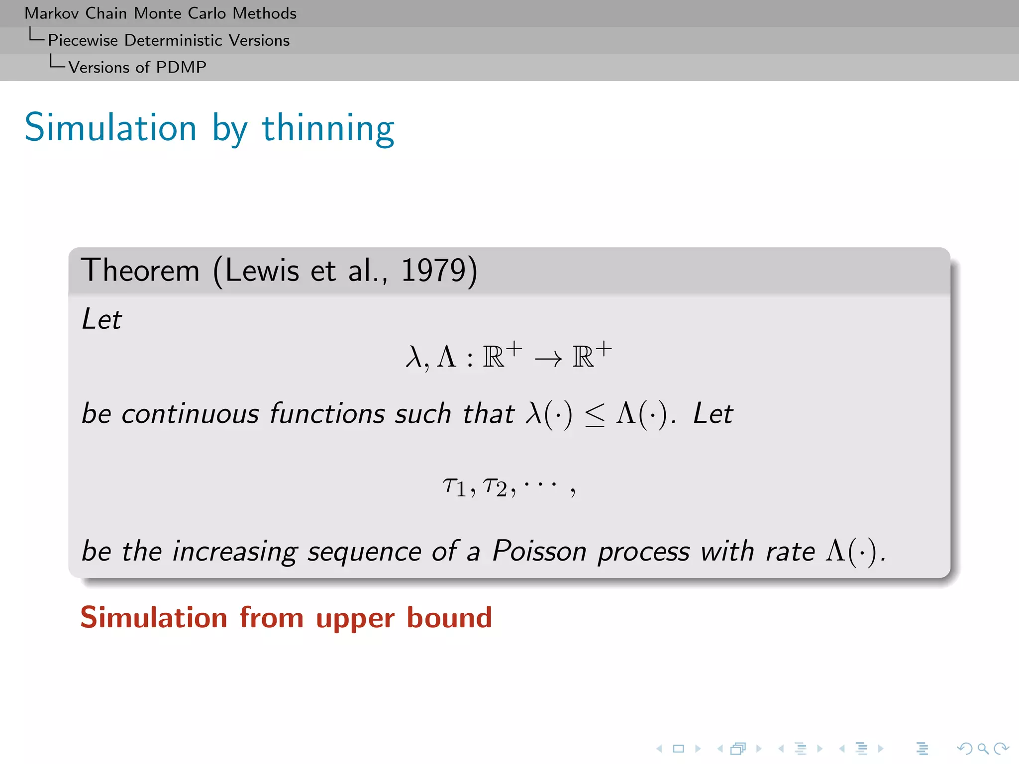
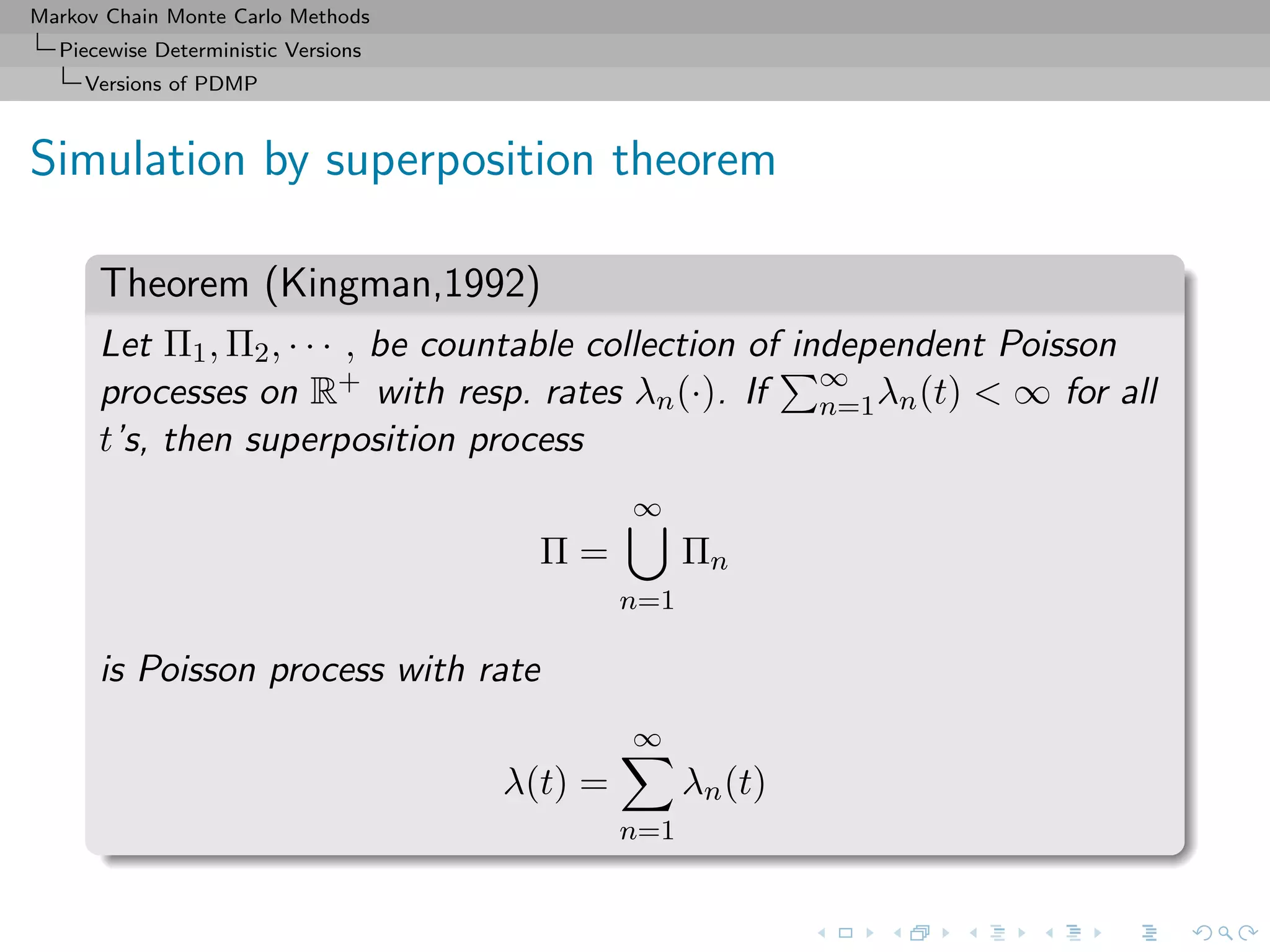
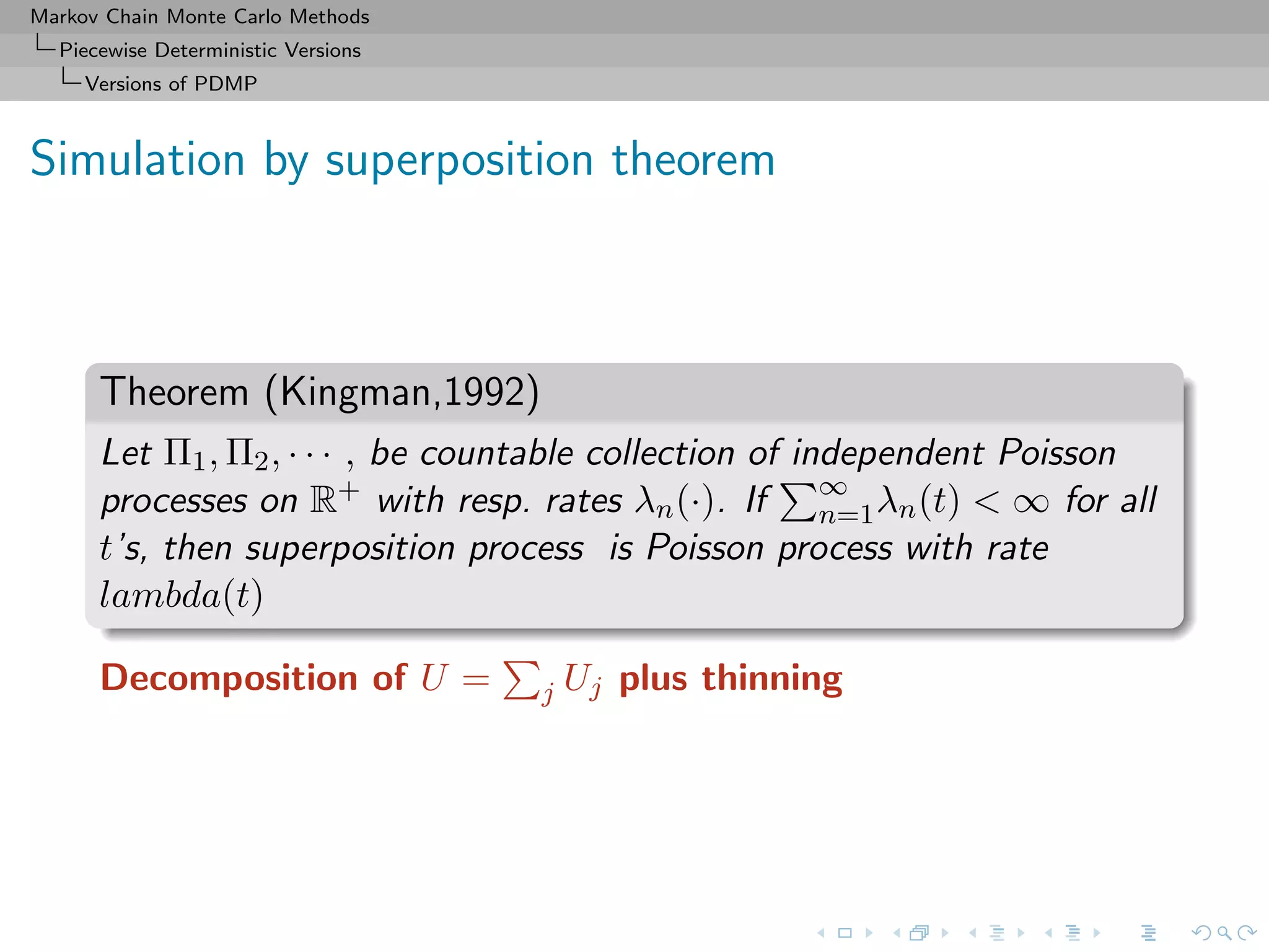
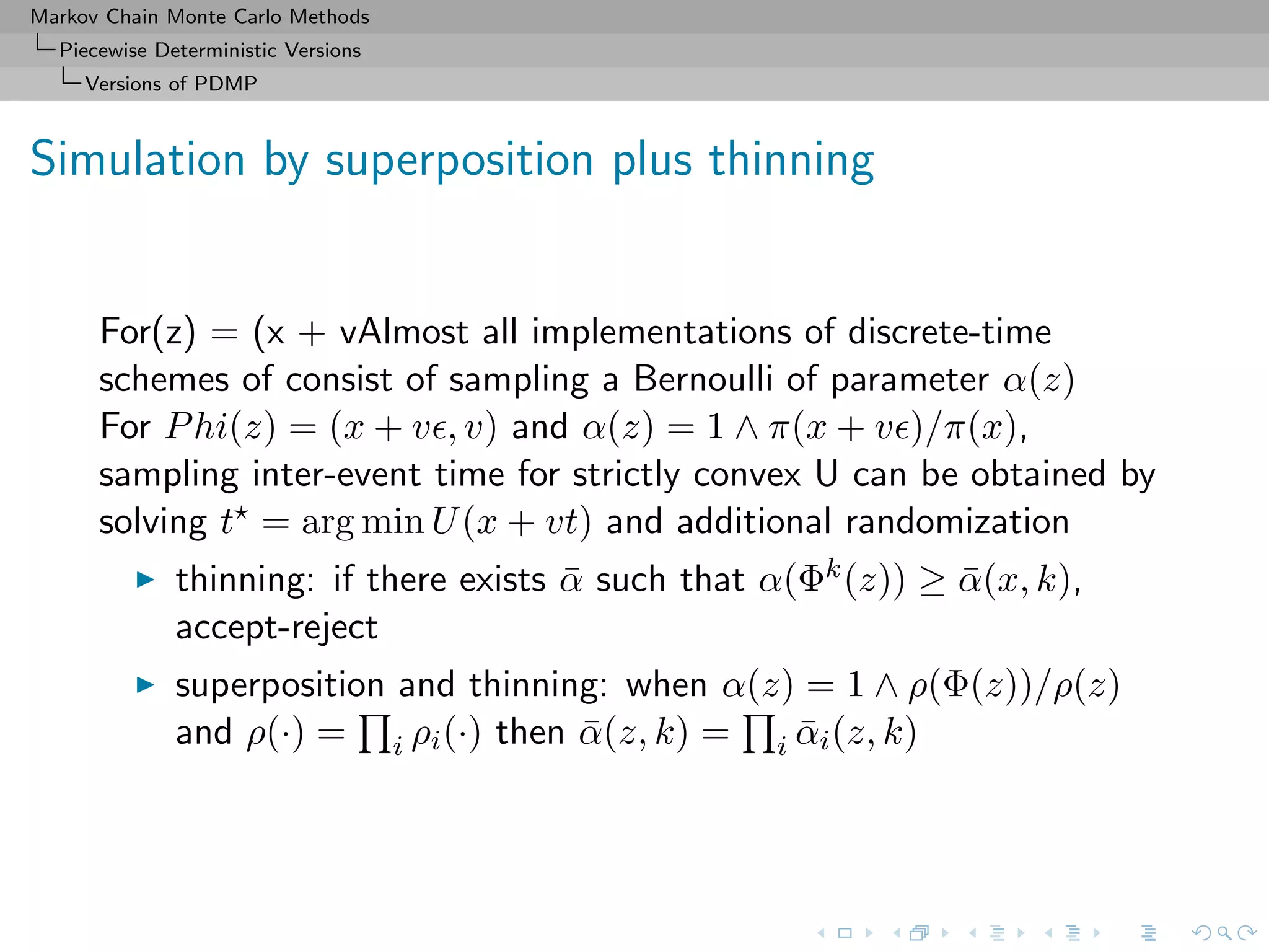
2. Simulating the inter-event time ηk: many techniques of
superposition and thinning for Poisson processes
[Devroye, 1986]](https://image.slidesharecdn.com/cirm-181022142714/75/short-course-at-CIRM-Bayesian-Masterclass-October-2018-180-2048.jpg)


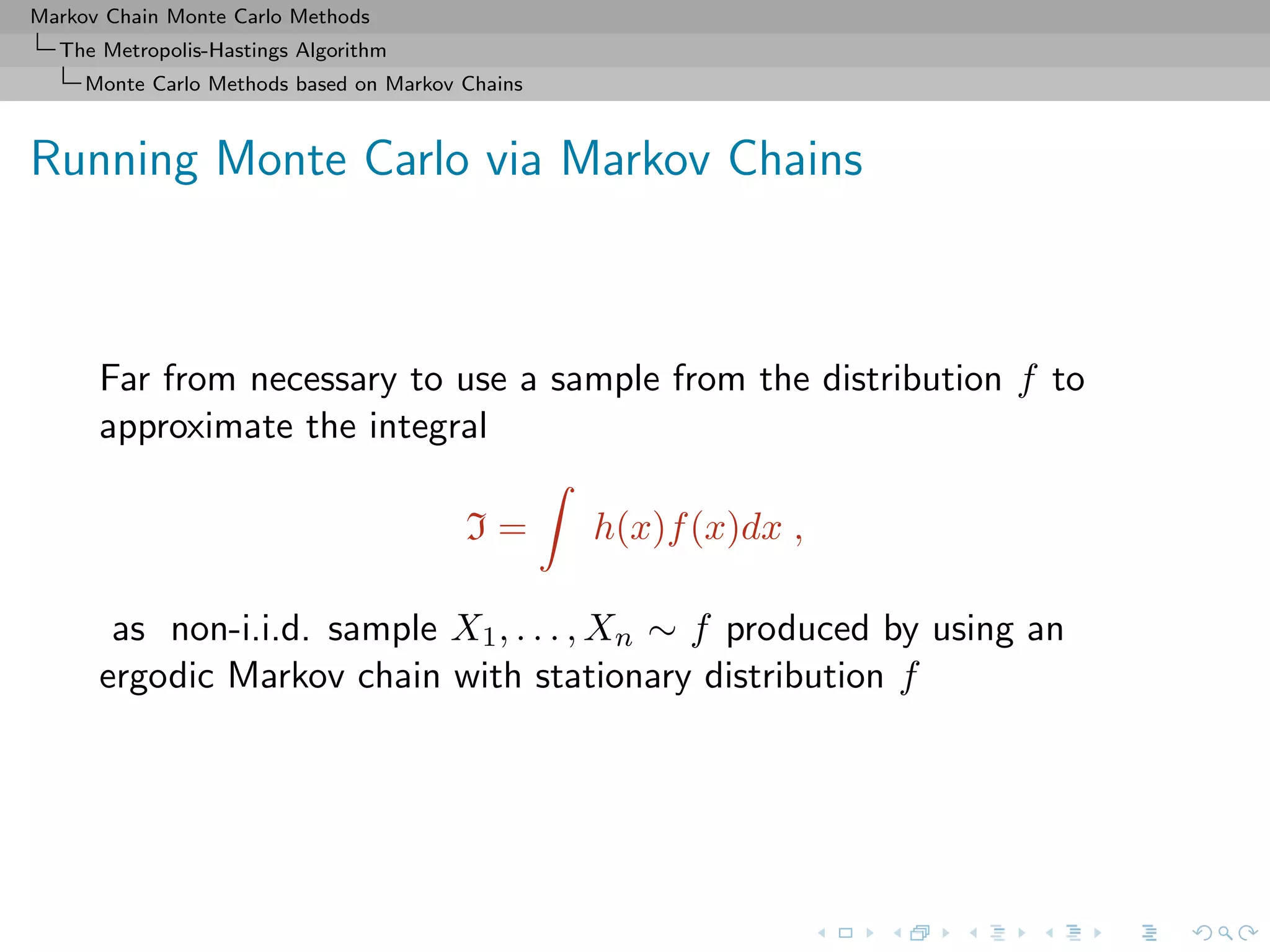
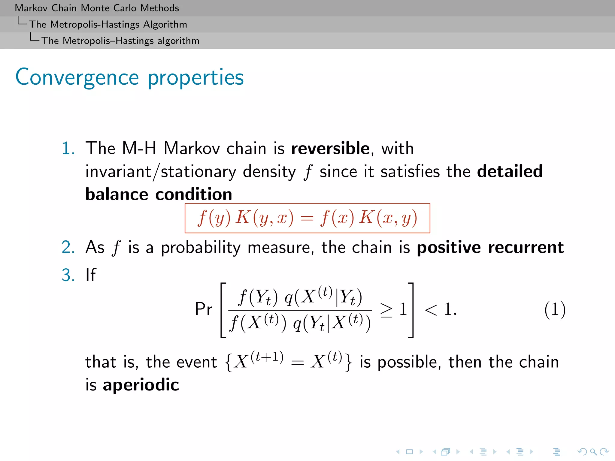
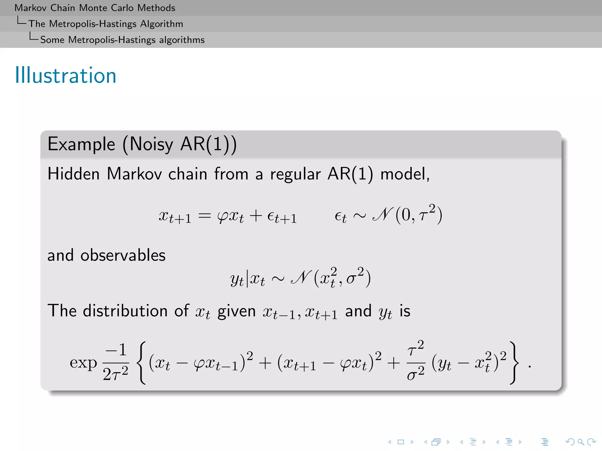
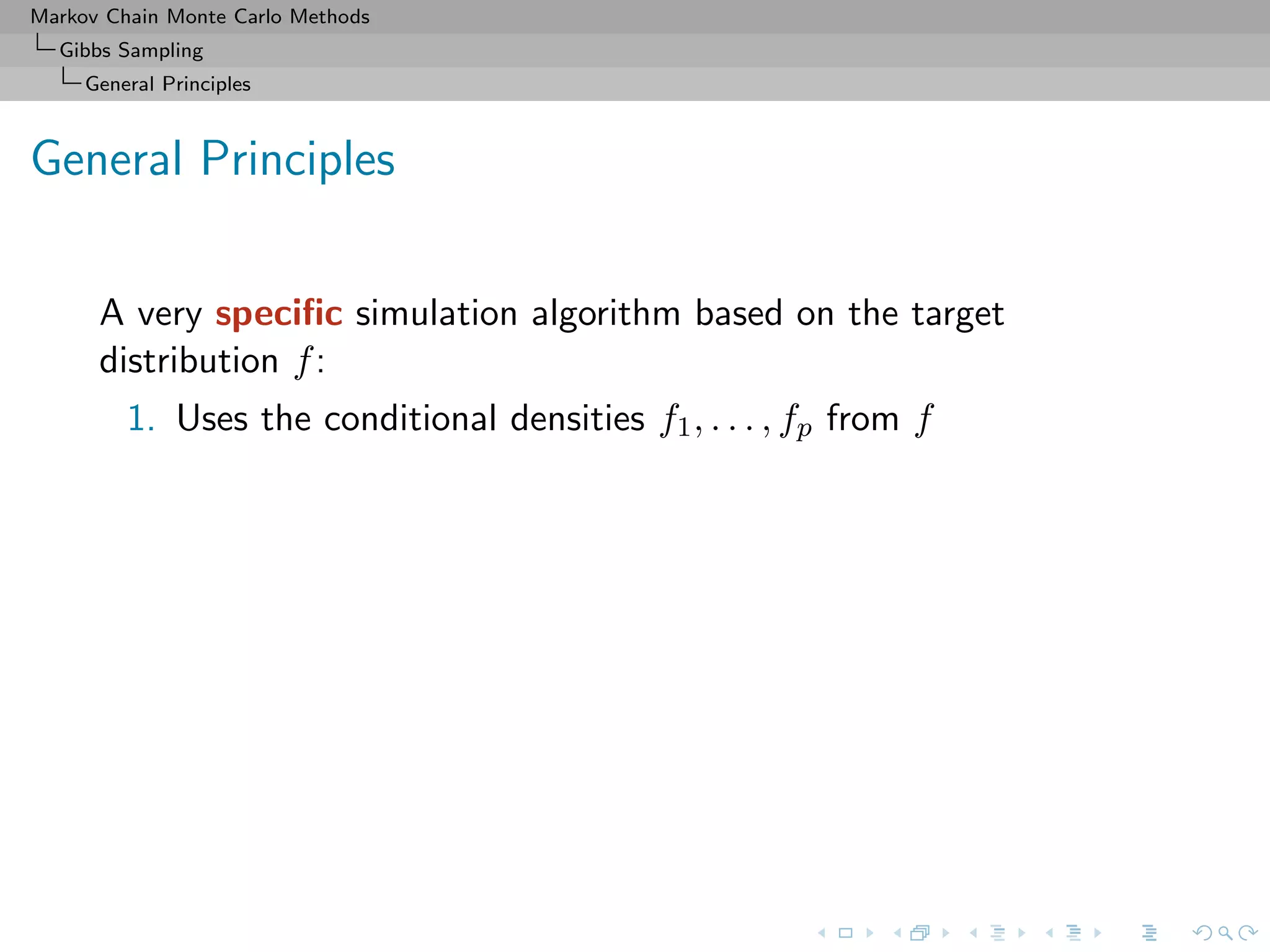
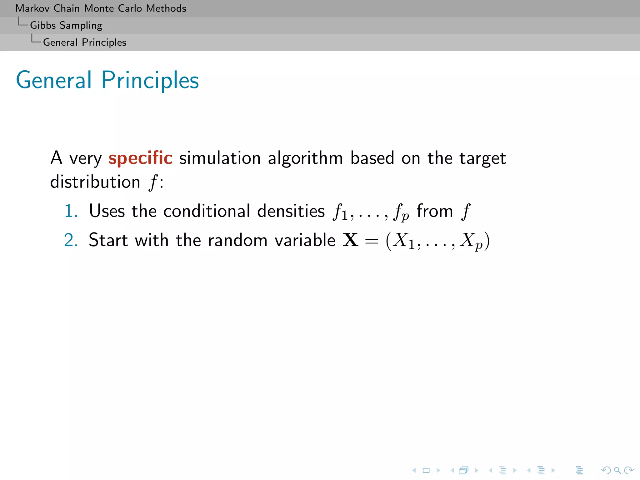
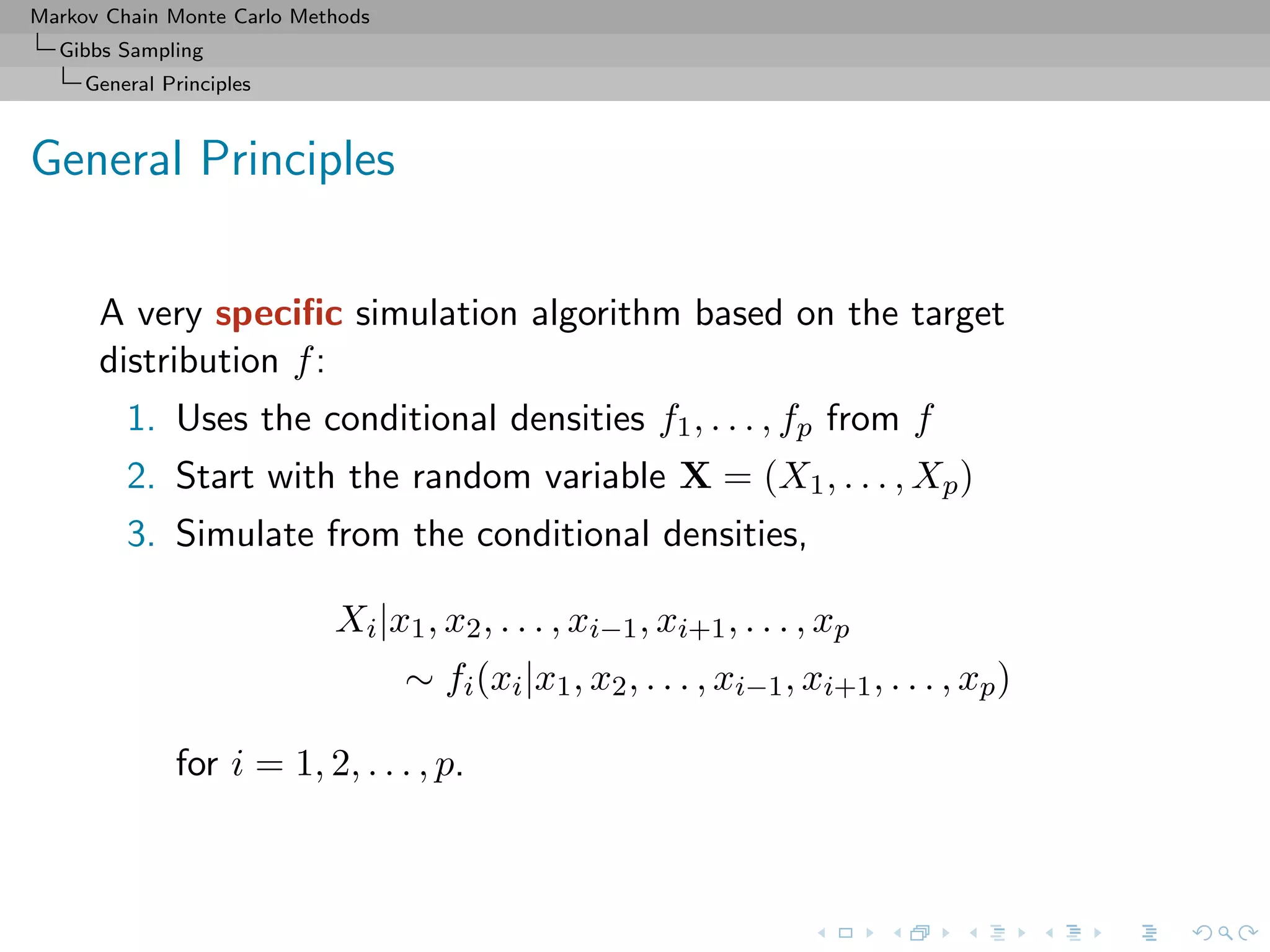
Markov Chain Monte Carlo (MCMC) methods generate dependent samples from a target distribution using a Markov chain. The Metropolis-Hastings algorithm constructs a Markov chain with a desired stationary distribution by proposing moves to new states and accepting or rejecting them probabilistically. The algorithm is used to approximate integrals that are difficult to compute directly. It has been shown to converge to the target distribution as the number of iterations increases.