Download as PDF, PPTX

![Outline
Unavailable likelihoods
ABC methods
ABC as an inference machine
[A]BCel
Conclusion and perspectives](https://image.slidesharecdn.com/i-like-130515231914-phpapp01/85/slides-of-ABC-talk-at-i-like-workshop-Warwick-May-16-3-320.jpg)


![summary as an answer to Lange, Chi & Zhou [ISR, 2013]
“Surprisingly, the confident prediction of the previous generation that Bayesian methods would
ultimately supplant frequentist methods has given way to a realization that Markov chain Monte
Carlo (MCMC) may be too slow to handle modern data sets. Size matters because large data sets
stress computer storage and processing power to the breaking point. The most successful
compromises between Bayesian and frequentist methods now rely on penalization and
optimization.”
sad reality constraint that size does matter
focus on much smaller dimensions and on sparse summaries
many (fast) ways of producing those summaries
Bayesian inference can kick in almost automatically at this
stage](https://image.slidesharecdn.com/i-like-130515231914-phpapp01/85/slides-of-ABC-talk-at-i-like-workshop-Warwick-May-16-12-320.jpg)
![summary as an answer to Lange, Chi & Zhou [ISR, 2013]
“Surprisingly, the confident prediction of the previous generation that Bayesian methods would
ultimately supplant frequentist methods has given way to a realization that Markov chain Monte
Carlo (MCMC) may be too slow to handle modern data sets. Size matters because large data sets
stress computer storage and processing power to the breaking point. The most successful
compromises between Bayesian and frequentist methods now rely on penalization and
optimization.”
sad reality constraint that size does matter
focus on much smaller dimensions and on sparse summaries
many (fast) ways of producing those summaries
Bayesian inference can kick in almost automatically at this
stage](https://image.slidesharecdn.com/i-like-130515231914-phpapp01/85/slides-of-ABC-talk-at-i-like-workshop-Warwick-May-16-13-320.jpg)
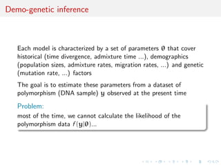
![Econom’ections
Similar exploration of simulation-based and approximation
techniques in Econometrics
Simulated method of moments
Method of simulated moments
Simulated pseudo-maximum-likelihood
Indirect inference
[Gouri´eroux & Monfort, 1996]
even though motivation is partly-defined models rather than
complex likelihoods](https://image.slidesharecdn.com/i-like-130515231914-phpapp01/85/slides-of-ABC-talk-at-i-like-workshop-Warwick-May-16-14-320.jpg)
![Econom’ections
Similar exploration of simulation-based and approximation
techniques in Econometrics
Simulated method of moments
Method of simulated moments
Simulated pseudo-maximum-likelihood
Indirect inference
[Gouri´eroux & Monfort, 1996]
even though motivation is partly-defined models rather than
complex likelihoods](https://image.slidesharecdn.com/i-like-130515231914-phpapp01/85/slides-of-ABC-talk-at-i-like-workshop-Warwick-May-16-15-320.jpg)
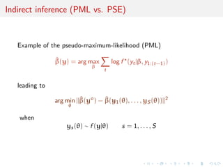
![Indirect inference
Minimise [in θ] a distance between estimators ^β based on a
pseudo-model for genuine observations and for observations
simulated under the true model and the parameter θ.
[Gouri´eroux, Monfort, & Renault, 1993;
Smith, 1993; Gallant & Tauchen, 1996]](https://image.slidesharecdn.com/i-like-130515231914-phpapp01/85/slides-of-ABC-talk-at-i-like-workshop-Warwick-May-16-16-320.jpg)
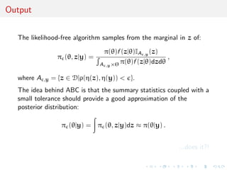
![Consistent indirect inference
“...in order to get a unique solution the dimension of
the auxiliary parameter β must be larger than or equal to
the dimension of the initial parameter θ. If the problem is
just identified the different methods become easier...”
Consistency depending on the criterion and on the asymptotic
identifiability of θ
[Gouri´eroux & Monfort, 1996, p. 66]
Which connection [if any] with the B perspective?](https://image.slidesharecdn.com/i-like-130515231914-phpapp01/85/slides-of-ABC-talk-at-i-like-workshop-Warwick-May-16-19-320.jpg)
![Consistent indirect inference
“...in order to get a unique solution the dimension of
the auxiliary parameter β must be larger than or equal to
the dimension of the initial parameter θ. If the problem is
just identified the different methods become easier...”
Consistency depending on the criterion and on the asymptotic
identifiability of θ
[Gouri´eroux & Monfort, 1996, p. 66]
Which connection [if any] with the B perspective?](https://image.slidesharecdn.com/i-like-130515231914-phpapp01/85/slides-of-ABC-talk-at-i-like-workshop-Warwick-May-16-20-320.jpg)
![Consistent indirect inference
“...in order to get a unique solution the dimension of
the auxiliary parameter β must be larger than or equal to
the dimension of the initial parameter θ. If the problem is
just identified the different methods become easier...”
Consistency depending on the criterion and on the asymptotic
identifiability of θ
[Gouri´eroux & Monfort, 1996, p. 66]
Which connection [if any] with the B perspective?](https://image.slidesharecdn.com/i-like-130515231914-phpapp01/85/slides-of-ABC-talk-at-i-like-workshop-Warwick-May-16-21-320.jpg)
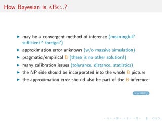
![Approximate Bayesian computation
Unavailable likelihoods
ABC methods
Genesis of ABC
ABC basics
Advances and interpretations
ABC as knn
ABC as an inference machine
[A]BCel
Conclusion and perspectives](https://image.slidesharecdn.com/i-like-130515231914-phpapp01/85/slides-of-ABC-talk-at-i-like-workshop-Warwick-May-16-22-320.jpg)
![Genetic background of ABC
skip genetics
ABC is a recent computational technique that only requires being
able to sample from the likelihood f (·|θ)
This technique stemmed from population genetics models, about
15 years ago, and population geneticists still contribute
significantly to methodological developments of ABC.
[Griffith & al., 1997; Tavar´e & al., 1999]](https://image.slidesharecdn.com/i-like-130515231914-phpapp01/85/slides-of-ABC-talk-at-i-like-workshop-Warwick-May-16-23-320.jpg)


![Intractable likelihood
Missing (too much missing!) data structure:
f (y|θ) =
G
f (y|G, θ)f (G|θ)dG
cannot be computed in a manageable way...
[Stephens & Donnelly, 2000]
The genealogies are considered as nuisance parameters
This modelling clearly differs from the phylogenetic perspective
where the tree is the parameter of interest.](https://image.slidesharecdn.com/i-like-130515231914-phpapp01/85/slides-of-ABC-talk-at-i-like-workshop-Warwick-May-16-31-320.jpg)
![Intractable likelihood
Missing (too much missing!) data structure:
f (y|θ) =
G
f (y|G, θ)f (G|θ)dG
cannot be computed in a manageable way...
[Stephens & Donnelly, 2000]
The genealogies are considered as nuisance parameters
This modelling clearly differs from the phylogenetic perspective
where the tree is the parameter of interest.](https://image.slidesharecdn.com/i-like-130515231914-phpapp01/85/slides-of-ABC-talk-at-i-like-workshop-Warwick-May-16-32-320.jpg)
![A?B?C?
A stands for approximate
[wrong likelihood / pic?]
B stands for Bayesian
C stands for computation
[producing a parameter
sample]](https://image.slidesharecdn.com/i-like-130515231914-phpapp01/85/slides-of-ABC-talk-at-i-like-workshop-Warwick-May-16-33-320.jpg)
![A?B?C?
A stands for approximate
[wrong likelihood / pic?]
B stands for Bayesian
C stands for computation
[producing a parameter
sample]](https://image.slidesharecdn.com/i-like-130515231914-phpapp01/85/slides-of-ABC-talk-at-i-like-workshop-Warwick-May-16-34-320.jpg)
![A?B?C?
A stands for approximate
[wrong likelihood / pic?]
B stands for Bayesian
C stands for computation
[producing a parameter
sample]
ESS=155.6
θ
Density
−0.5 0.0 0.5 1.0
0.01.0
ESS=75.93
θ
Density
−0.4 −0.2 0.0 0.2 0.4
0.01.02.0
ESS=76.87
θ
Density
−0.4 −0.2 0.0 0.2
01234
ESS=91.54
θ
Density
−0.6 −0.4 −0.2 0.0 0.2
01234
ESS=108.4
θ
Density
−0.4 0.0 0.2 0.4 0.6
0.01.02.03.0
ESS=85.13
θ
Density
−0.2 0.0 0.2 0.4 0.6
0.01.02.03.0
ESS=149.1
θ
Density
−0.5 0.0 0.5 1.0
0.01.02.0
ESS=96.31
θ
Density
−0.4 0.0 0.2 0.4 0.6
0.01.02.0
ESS=83.77
θ
Density
−0.6 −0.4 −0.2 0.0 0.2 0.4
01234
ESS=155.7
θ
Density
−0.5 0.0 0.5
0.01.02.0
ESS=92.42
θ
Density
−0.4 0.0 0.2 0.4 0.6
0.01.02.03.0
ESS=95.01
θ
Density
−0.4 0.0 0.2 0.4 0.6
0.01.53.0
ESS=139.2
Density −0.6 −0.2 0.2 0.6
0.01.02.0
ESS=99.33
Density
−0.4 −0.2 0.0 0.2 0.4
0.01.02.03.0
ESS=87.28
Density
−0.2 0.0 0.2 0.4 0.6
0123](https://image.slidesharecdn.com/i-like-130515231914-phpapp01/85/slides-of-ABC-talk-at-i-like-workshop-Warwick-May-16-35-320.jpg)

![ABC methodology
Bayesian setting: target is π(θ)f (x|θ)
When likelihood f (x|θ) not in closed form, likelihood-free rejection
technique:
Foundation
For an observation y ∼ f (y|θ), under the prior π(θ), if one keeps
jointly simulating
θ ∼ π(θ) , z ∼ f (z|θ ) ,
until the auxiliary variable z is equal to the observed value, z = y,
then the selected
θ ∼ π(θ|y)
[Rubin, 1984; Diggle & Gratton, 1984; Tavar´e et al., 1997]](https://image.slidesharecdn.com/i-like-130515231914-phpapp01/85/slides-of-ABC-talk-at-i-like-workshop-Warwick-May-16-37-320.jpg)
![ABC methodology
Bayesian setting: target is π(θ)f (x|θ)
When likelihood f (x|θ) not in closed form, likelihood-free rejection
technique:
Foundation
For an observation y ∼ f (y|θ), under the prior π(θ), if one keeps
jointly simulating
θ ∼ π(θ) , z ∼ f (z|θ ) ,
until the auxiliary variable z is equal to the observed value, z = y,
then the selected
θ ∼ π(θ|y)
[Rubin, 1984; Diggle & Gratton, 1984; Tavar´e et al., 1997]](https://image.slidesharecdn.com/i-like-130515231914-phpapp01/85/slides-of-ABC-talk-at-i-like-workshop-Warwick-May-16-38-320.jpg)
![ABC methodology
Bayesian setting: target is π(θ)f (x|θ)
When likelihood f (x|θ) not in closed form, likelihood-free rejection
technique:
Foundation
For an observation y ∼ f (y|θ), under the prior π(θ), if one keeps
jointly simulating
θ ∼ π(θ) , z ∼ f (z|θ ) ,
until the auxiliary variable z is equal to the observed value, z = y,
then the selected
θ ∼ π(θ|y)
[Rubin, 1984; Diggle & Gratton, 1984; Tavar´e et al., 1997]](https://image.slidesharecdn.com/i-like-130515231914-phpapp01/85/slides-of-ABC-talk-at-i-like-workshop-Warwick-May-16-39-320.jpg)
![A as A...pproximative
When y is a continuous random variable, strict equality z = y is
replaced with a tolerance zone
ρ(y, z)
where ρ is a distance
Output distributed from
π(θ) Pθ{ρ(y, z) < }
def
∝ π(θ|ρ(y, z) < )
[Pritchard et al., 1999]](https://image.slidesharecdn.com/i-like-130515231914-phpapp01/85/slides-of-ABC-talk-at-i-like-workshop-Warwick-May-16-40-320.jpg)
![A as A...pproximative
When y is a continuous random variable, strict equality z = y is
replaced with a tolerance zone
ρ(y, z)
where ρ is a distance
Output distributed from
π(θ) Pθ{ρ(y, z) < }
def
∝ π(θ|ρ(y, z) < )
[Pritchard et al., 1999]](https://image.slidesharecdn.com/i-like-130515231914-phpapp01/85/slides-of-ABC-talk-at-i-like-workshop-Warwick-May-16-41-320.jpg)


![ABC (simul’) advances
how approximative is ABC? ABC as knn
Simulating from the prior is often poor in efficiency
Either modify the proposal distribution on θ to increase the density
of x’s within the vicinity of y...
[Marjoram et al, 2003; Bortot et al., 2007, Sisson et al., 2007]
...or by viewing the problem as a conditional density estimation
and by developing techniques to allow for larger
[Beaumont et al., 2002]
.....or even by including in the inferential framework [ABCµ]
[Ratmann et al., 2009]](https://image.slidesharecdn.com/i-like-130515231914-phpapp01/85/slides-of-ABC-talk-at-i-like-workshop-Warwick-May-16-53-320.jpg)
![ABC (simul’) advances
how approximative is ABC? ABC as knn
Simulating from the prior is often poor in efficiency
Either modify the proposal distribution on θ to increase the density
of x’s within the vicinity of y...
[Marjoram et al, 2003; Bortot et al., 2007, Sisson et al., 2007]
...or by viewing the problem as a conditional density estimation
and by developing techniques to allow for larger
[Beaumont et al., 2002]
.....or even by including in the inferential framework [ABCµ]
[Ratmann et al., 2009]](https://image.slidesharecdn.com/i-like-130515231914-phpapp01/85/slides-of-ABC-talk-at-i-like-workshop-Warwick-May-16-54-320.jpg)
![ABC (simul’) advances
how approximative is ABC? ABC as knn
Simulating from the prior is often poor in efficiency
Either modify the proposal distribution on θ to increase the density
of x’s within the vicinity of y...
[Marjoram et al, 2003; Bortot et al., 2007, Sisson et al., 2007]
...or by viewing the problem as a conditional density estimation
and by developing techniques to allow for larger
[Beaumont et al., 2002]
.....or even by including in the inferential framework [ABCµ]
[Ratmann et al., 2009]](https://image.slidesharecdn.com/i-like-130515231914-phpapp01/85/slides-of-ABC-talk-at-i-like-workshop-Warwick-May-16-55-320.jpg)
![ABC (simul’) advances
how approximative is ABC? ABC as knn
Simulating from the prior is often poor in efficiency
Either modify the proposal distribution on θ to increase the density
of x’s within the vicinity of y...
[Marjoram et al, 2003; Bortot et al., 2007, Sisson et al., 2007]
...or by viewing the problem as a conditional density estimation
and by developing techniques to allow for larger
[Beaumont et al., 2002]
.....or even by including in the inferential framework [ABCµ]
[Ratmann et al., 2009]](https://image.slidesharecdn.com/i-like-130515231914-phpapp01/85/slides-of-ABC-talk-at-i-like-workshop-Warwick-May-16-56-320.jpg)
![ABC-NP
Better usage of [prior] simulations by
adjustement: instead of throwing away
θ such that ρ(η(z), η(y)) > , replace
θ’s with locally regressed transforms
θ∗
= θ − {η(z) − η(y)}T ^β
[Csill´ery et al., TEE, 2010]
where ^β is obtained by [NP] weighted least square regression on
(η(z) − η(y)) with weights
Kδ {ρ(η(z), η(y))}
[Beaumont et al., 2002, Genetics]](https://image.slidesharecdn.com/i-like-130515231914-phpapp01/85/slides-of-ABC-talk-at-i-like-workshop-Warwick-May-16-57-320.jpg)
![ABC-NP (regression)
Also found in the subsequent literature, e.g. in Fearnhead-Prangle (2012) :
weight directly simulation by
Kδ {ρ(η(z(θ)), η(y))}
or
1
S
S
s=1
Kδ {ρ(η(zs
(θ)), η(y))}
[consistent estimate of f (η|θ)]
Curse of dimensionality: poor estimate when d = dim(η) is large...](https://image.slidesharecdn.com/i-like-130515231914-phpapp01/85/slides-of-ABC-talk-at-i-like-workshop-Warwick-May-16-58-320.jpg)
![ABC-NP (regression)
Also found in the subsequent literature, e.g. in Fearnhead-Prangle (2012) :
weight directly simulation by
Kδ {ρ(η(z(θ)), η(y))}
or
1
S
S
s=1
Kδ {ρ(η(zs
(θ)), η(y))}
[consistent estimate of f (η|θ)]
Curse of dimensionality: poor estimate when d = dim(η) is large...](https://image.slidesharecdn.com/i-like-130515231914-phpapp01/85/slides-of-ABC-talk-at-i-like-workshop-Warwick-May-16-59-320.jpg)
![ABC-NP (density estimation)
Use of the kernel weights
Kδ {ρ(η(z(θ)), η(y))}
leads to the NP estimate of the posterior expectation
i θi Kδ {ρ(η(z(θi )), η(y))}
i Kδ {ρ(η(z(θi )), η(y))}
[Blum, JASA, 2010]](https://image.slidesharecdn.com/i-like-130515231914-phpapp01/85/slides-of-ABC-talk-at-i-like-workshop-Warwick-May-16-60-320.jpg)
![ABC-NP (density estimation)
Use of the kernel weights
Kδ {ρ(η(z(θ)), η(y))}
leads to the NP estimate of the posterior conditional density
i
˜Kb(θi − θ)Kδ {ρ(η(z(θi )), η(y))}
i Kδ {ρ(η(z(θi )), η(y))}
[Blum, JASA, 2010]](https://image.slidesharecdn.com/i-like-130515231914-phpapp01/85/slides-of-ABC-talk-at-i-like-workshop-Warwick-May-16-61-320.jpg)
![ABC-NP (density estimations)
Other versions incorporating regression adjustments
i
˜Kb(θ∗
i − θ)Kδ {ρ(η(z(θi )), η(y))}
i Kδ {ρ(η(z(θi )), η(y))}
In all cases, error
E[^g(θ|y)] − g(θ|y) = cb2
+ cδ2
+ OP(b2
+ δ2
) + OP(1/nδd
)
var(^g(θ|y)) =
c
nbδd
(1 + oP(1))](https://image.slidesharecdn.com/i-like-130515231914-phpapp01/85/slides-of-ABC-talk-at-i-like-workshop-Warwick-May-16-62-320.jpg)
![ABC-NP (density estimations)
Other versions incorporating regression adjustments
i
˜Kb(θ∗
i − θ)Kδ {ρ(η(z(θi )), η(y))}
i Kδ {ρ(η(z(θi )), η(y))}
In all cases, error
E[^g(θ|y)] − g(θ|y) = cb2
+ cδ2
+ OP(b2
+ δ2
) + OP(1/nδd
)
var(^g(θ|y)) =
c
nbδd
(1 + oP(1))
[Blum, JASA, 2010]](https://image.slidesharecdn.com/i-like-130515231914-phpapp01/85/slides-of-ABC-talk-at-i-like-workshop-Warwick-May-16-63-320.jpg)
![ABC-NP (density estimations)
Other versions incorporating regression adjustments
i
˜Kb(θ∗
i − θ)Kδ {ρ(η(z(θi )), η(y))}
i Kδ {ρ(η(z(θi )), η(y))}
In all cases, error
E[^g(θ|y)] − g(θ|y) = cb2
+ cδ2
+ OP(b2
+ δ2
) + OP(1/nδd
)
var(^g(θ|y)) =
c
nbδd
(1 + oP(1))
[standard NP calculations]](https://image.slidesharecdn.com/i-like-130515231914-phpapp01/85/slides-of-ABC-talk-at-i-like-workshop-Warwick-May-16-64-320.jpg)
![ABC as knn
[Biau et al., 2013, Annales de l’IHP]
Practice of ABC: determine tolerance as a quantile on observed
distances, say 10% or 1% quantile,
= N = qα(d1, . . . , dN)
Interpretation of ε as nonparametric bandwidth only
approximation of the actual practice
[Blum & Fran¸cois, 2010]
ABC is a k-nearest neighbour (knn) method with kN = N N
[Loftsgaarden & Quesenberry, 1965]](https://image.slidesharecdn.com/i-like-130515231914-phpapp01/85/slides-of-ABC-talk-at-i-like-workshop-Warwick-May-16-65-320.jpg)
![ABC as knn
[Biau et al., 2013, Annales de l’IHP]
Practice of ABC: determine tolerance as a quantile on observed
distances, say 10% or 1% quantile,
= N = qα(d1, . . . , dN)
Interpretation of ε as nonparametric bandwidth only
approximation of the actual practice
[Blum & Fran¸cois, 2010]
ABC is a k-nearest neighbour (knn) method with kN = N N
[Loftsgaarden & Quesenberry, 1965]](https://image.slidesharecdn.com/i-like-130515231914-phpapp01/85/slides-of-ABC-talk-at-i-like-workshop-Warwick-May-16-66-320.jpg)
![ABC as knn
[Biau et al., 2013, Annales de l’IHP]
Practice of ABC: determine tolerance as a quantile on observed
distances, say 10% or 1% quantile,
= N = qα(d1, . . . , dN)
Interpretation of ε as nonparametric bandwidth only
approximation of the actual practice
[Blum & Fran¸cois, 2010]
ABC is a k-nearest neighbour (knn) method with kN = N N
[Loftsgaarden & Quesenberry, 1965]](https://image.slidesharecdn.com/i-like-130515231914-phpapp01/85/slides-of-ABC-talk-at-i-like-workshop-Warwick-May-16-67-320.jpg)
![ABC consistency
Provided
kN/ log log N −→ ∞ and kN/N −→ 0
as N → ∞, for almost all s0 (with respect to the distribution of
S), with probability 1,
1
kN
kN
j=1
ϕ(θj ) −→ E[ϕ(θj )|S = s0]
[Devroye, 1982]
Biau et al. (2012) also recall pointwise and integrated mean square error
consistency results on the corresponding kernel estimate of the
conditional posterior distribution, under constraints
kN → ∞, kN /N → 0, hN → 0 and hp
N kN → ∞,](https://image.slidesharecdn.com/i-like-130515231914-phpapp01/85/slides-of-ABC-talk-at-i-like-workshop-Warwick-May-16-68-320.jpg)
![ABC consistency
Provided
kN/ log log N −→ ∞ and kN/N −→ 0
as N → ∞, for almost all s0 (with respect to the distribution of
S), with probability 1,
1
kN
kN
j=1
ϕ(θj ) −→ E[ϕ(θj )|S = s0]
[Devroye, 1982]
Biau et al. (2012) also recall pointwise and integrated mean square error
consistency results on the corresponding kernel estimate of the
conditional posterior distribution, under constraints
kN → ∞, kN /N → 0, hN → 0 and hp
N kN → ∞,](https://image.slidesharecdn.com/i-like-130515231914-phpapp01/85/slides-of-ABC-talk-at-i-like-workshop-Warwick-May-16-69-320.jpg)
![Rates of convergence
Further assumptions (on target and kernel) allow for precise
(integrated mean square) convergence rates (as a power of the
sample size N), derived from classical k-nearest neighbour
regression, like
when m = 1, 2, 3, kN ≈ N(p+4)/(p+8) and rate N− 4
p+8
when m = 4, kN ≈ N(p+4)/(p+8) and rate N− 4
p+8 log N
when m > 4, kN ≈ N(p+4)/(m+p+4) and rate N− 4
m+p+4
[Biau et al., 2012, arxiv:1207.6461]
Drag: Only applies to sufficient summary statistics](https://image.slidesharecdn.com/i-like-130515231914-phpapp01/85/slides-of-ABC-talk-at-i-like-workshop-Warwick-May-16-70-320.jpg)
![Rates of convergence
Further assumptions (on target and kernel) allow for precise
(integrated mean square) convergence rates (as a power of the
sample size N), derived from classical k-nearest neighbour
regression, like
when m = 1, 2, 3, kN ≈ N(p+4)/(p+8) and rate N− 4
p+8
when m = 4, kN ≈ N(p+4)/(p+8) and rate N− 4
p+8 log N
when m > 4, kN ≈ N(p+4)/(m+p+4) and rate N− 4
m+p+4
[Biau et al., 2012, arxiv:1207.6461]
Drag: Only applies to sufficient summary statistics](https://image.slidesharecdn.com/i-like-130515231914-phpapp01/85/slides-of-ABC-talk-at-i-like-workshop-Warwick-May-16-71-320.jpg)
![ABC inference machine
Unavailable likelihoods
ABC methods
ABC as an inference machine
Error inc.
Exact BC and approximate
targets
summary statistic
[A]BCel
Conclusion and perspectives](https://image.slidesharecdn.com/i-like-130515231914-phpapp01/85/slides-of-ABC-talk-at-i-like-workshop-Warwick-May-16-72-320.jpg)
![ABCµ
Idea Infer about the error as well as about the parameter:
Use of a joint density
f (θ, |y) ∝ ξ( |y, θ) × πθ(θ) × π ( )
where y is the data, and ξ( |y, θ) is the prior predictive density of
ρ(η(z), η(y)) given θ and y when z ∼ f (z|θ)
Warning! Replacement of ξ( |y, θ) with a non-parametric kernel
approximation.
[Ratmann, Andrieu, Wiuf and Richardson, 2009, PNAS]](https://image.slidesharecdn.com/i-like-130515231914-phpapp01/85/slides-of-ABC-talk-at-i-like-workshop-Warwick-May-16-74-320.jpg)
![ABCµ
Idea Infer about the error as well as about the parameter:
Use of a joint density
f (θ, |y) ∝ ξ( |y, θ) × πθ(θ) × π ( )
where y is the data, and ξ( |y, θ) is the prior predictive density of
ρ(η(z), η(y)) given θ and y when z ∼ f (z|θ)
Warning! Replacement of ξ( |y, θ) with a non-parametric kernel
approximation.
[Ratmann, Andrieu, Wiuf and Richardson, 2009, PNAS]](https://image.slidesharecdn.com/i-like-130515231914-phpapp01/85/slides-of-ABC-talk-at-i-like-workshop-Warwick-May-16-75-320.jpg)
![ABCµ
Idea Infer about the error as well as about the parameter:
Use of a joint density
f (θ, |y) ∝ ξ( |y, θ) × πθ(θ) × π ( )
where y is the data, and ξ( |y, θ) is the prior predictive density of
ρ(η(z), η(y)) given θ and y when z ∼ f (z|θ)
Warning! Replacement of ξ( |y, θ) with a non-parametric kernel
approximation.
[Ratmann, Andrieu, Wiuf and Richardson, 2009, PNAS]](https://image.slidesharecdn.com/i-like-130515231914-phpapp01/85/slides-of-ABC-talk-at-i-like-workshop-Warwick-May-16-76-320.jpg)
![ABCµ details
Multidimensional distances ρk (k = 1, . . . , K) and errors
k = ρk(ηk(z), ηk(y)), with
k ∼ ξk( |y, θ) ≈ ^ξk( |y, θ) =
1
Bhk
b
K[{ k−ρk(ηk(zb), ηk(y))}/hk]
then used in replacing ξ( |y, θ) with mink
^ξk( |y, θ)
ABCµ involves acceptance probability
π(θ , )
π(θ, )
q(θ , θ)q( , )
q(θ, θ )q( , )
mink
^ξk( |y, θ )
mink
^ξk( |y, θ)](https://image.slidesharecdn.com/i-like-130515231914-phpapp01/85/slides-of-ABC-talk-at-i-like-workshop-Warwick-May-16-77-320.jpg)
![ABCµ details
Multidimensional distances ρk (k = 1, . . . , K) and errors
k = ρk(ηk(z), ηk(y)), with
k ∼ ξk( |y, θ) ≈ ^ξk( |y, θ) =
1
Bhk
b
K[{ k−ρk(ηk(zb), ηk(y))}/hk]
then used in replacing ξ( |y, θ) with mink
^ξk( |y, θ)
ABCµ involves acceptance probability
π(θ , )
π(θ, )
q(θ , θ)q( , )
q(θ, θ )q( , )
mink
^ξk( |y, θ )
mink
^ξk( |y, θ)](https://image.slidesharecdn.com/i-like-130515231914-phpapp01/85/slides-of-ABC-talk-at-i-like-workshop-Warwick-May-16-78-320.jpg)
![Wilkinson’s exact BC (not exactly!)
ABC approximation error (i.e. non-zero tolerance) replaced with
exact simulation from a controlled approximation to the target,
convolution of true posterior with kernel function
π (θ, z|y) =
π(θ)f (z|θ)K (y − z)
π(θ)f (z|θ)K (y − z)dzdθ
,
with K kernel parameterised by bandwidth .
[Wilkinson, 2013]
Theorem
The ABC algorithm based on the assumption of a randomised
observation y = ˜y + ξ, ξ ∼ K , and an acceptance probability of
K (y − z)/M
gives draws from the posterior distribution π(θ|y).](https://image.slidesharecdn.com/i-like-130515231914-phpapp01/85/slides-of-ABC-talk-at-i-like-workshop-Warwick-May-16-79-320.jpg)
![Wilkinson’s exact BC (not exactly!)
ABC approximation error (i.e. non-zero tolerance) replaced with
exact simulation from a controlled approximation to the target,
convolution of true posterior with kernel function
π (θ, z|y) =
π(θ)f (z|θ)K (y − z)
π(θ)f (z|θ)K (y − z)dzdθ
,
with K kernel parameterised by bandwidth .
[Wilkinson, 2013]
Theorem
The ABC algorithm based on the assumption of a randomised
observation y = ˜y + ξ, ξ ∼ K , and an acceptance probability of
K (y − z)/M
gives draws from the posterior distribution π(θ|y).](https://image.slidesharecdn.com/i-like-130515231914-phpapp01/85/slides-of-ABC-talk-at-i-like-workshop-Warwick-May-16-80-320.jpg)
![How exact a BC?
Pros
Pseudo-data from true model and observed data from noisy
model
Interesting perspective in that outcome is completely
controlled
Link with ABCµ and assuming y is observed with a
measurement error with density K
Relates to the theory of model approximation
[Kennedy & O’Hagan, 2001]
leads to “noisy ABC”: perturbates the data down to precision
ε and proceed
[Fearnhead & Prangle, 2012]
Cons
Requires K to be bounded by M
True approximation error never assessed](https://image.slidesharecdn.com/i-like-130515231914-phpapp01/85/slides-of-ABC-talk-at-i-like-workshop-Warwick-May-16-81-320.jpg)
![How exact a BC?
Pros
Pseudo-data from true model and observed data from noisy
model
Interesting perspective in that outcome is completely
controlled
Link with ABCµ and assuming y is observed with a
measurement error with density K
Relates to the theory of model approximation
[Kennedy & O’Hagan, 2001]
leads to “noisy ABC”: perturbates the data down to precision
ε and proceed
[Fearnhead & Prangle, 2012]
Cons
Requires K to be bounded by M
True approximation error never assessed](https://image.slidesharecdn.com/i-like-130515231914-phpapp01/85/slides-of-ABC-talk-at-i-like-workshop-Warwick-May-16-82-320.jpg)
![Noisy ABC for HMMs
Specific case of a hidden Markov model summaries
Xt+1 ∼ Qθ(Xt, ·)
Yt+1 ∼ gθ(·|xt)
where only y0
1:n is observed.
[Dean, Singh, Jasra, & Peters, 2011]
Use of specific constraints, adapted to the Markov structure:
y1 ∈ B(y0
1 , ) × · · · × yn ∈ B(y0
n , )](https://image.slidesharecdn.com/i-like-130515231914-phpapp01/85/slides-of-ABC-talk-at-i-like-workshop-Warwick-May-16-83-320.jpg)
![Noisy ABC for HMMs
Specific case of a hidden Markov model summaries
Xt+1 ∼ Qθ(Xt, ·)
Yt+1 ∼ gθ(·|xt)
where only y0
1:n is observed.
[Dean, Singh, Jasra, & Peters, 2011]
Use of specific constraints, adapted to the Markov structure:
y1 ∈ B(y0
1 , ) × · · · × yn ∈ B(y0
n , )](https://image.slidesharecdn.com/i-like-130515231914-phpapp01/85/slides-of-ABC-talk-at-i-like-workshop-Warwick-May-16-84-320.jpg)
![Noisy ABC-MLE
Idea: Modify instead the data from the start
(y0
1 + ζ1, . . . , yn + ζn)
[ see Fearnhead-Prangle ]
noisy ABC-MLE estimate
arg max
θ
Pθ Y1 ∈ B(y0
1 + ζ1, ), . . . , Yn ∈ B(y0
n + ζn, )
[Dean, Singh, Jasra, & Peters, 2011]](https://image.slidesharecdn.com/i-like-130515231914-phpapp01/85/slides-of-ABC-talk-at-i-like-workshop-Warwick-May-16-85-320.jpg)
![Consistent noisy ABC-MLE
Degrading the data improves the estimation performances:
Noisy ABC-MLE is asymptotically (in n) consistent
under further assumptions, the noisy ABC-MLE is
asymptotically normal
increase in variance of order −2
likely degradation in precision or computing time due to the
lack of summary statistic [curse of dimensionality]](https://image.slidesharecdn.com/i-like-130515231914-phpapp01/85/slides-of-ABC-talk-at-i-like-workshop-Warwick-May-16-86-320.jpg)


![Which summary for model choice?
Depending on the choice of η(·), the Bayes factor based on this
insufficient statistic,
Bη
12(y) =
π1(θ1)f η
1 (η(y)|θ1) dθ1
π2(θ2)f η
2 (η(y)|θ2) dθ2
,
is either consistent or inconsistent
[X, Cornuet, Marin, & Pillai, 2012]
Consistency only depends on the range of Ei [η(y)] under both
models
[Marin, Pillai, X, & Rousseau, 2012]](https://image.slidesharecdn.com/i-like-130515231914-phpapp01/85/slides-of-ABC-talk-at-i-like-workshop-Warwick-May-16-90-320.jpg)
![Which summary for model choice?
Depending on the choice of η(·), the Bayes factor based on this
insufficient statistic,
Bη
12(y) =
π1(θ1)f η
1 (η(y)|θ1) dθ1
π2(θ2)f η
2 (η(y)|θ2) dθ2
,
is either consistent or inconsistent
[X, Cornuet, Marin, & Pillai, 2012]
Consistency only depends on the range of Ei [η(y)] under both
models
[Marin, Pillai, X, & Rousseau, 2012]](https://image.slidesharecdn.com/i-like-130515231914-phpapp01/85/slides-of-ABC-talk-at-i-like-workshop-Warwick-May-16-91-320.jpg)
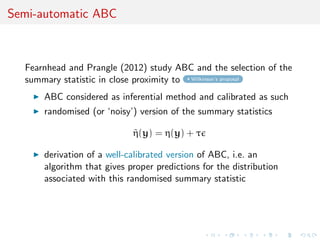
![Summary [of F&P/statistics)
optimality of the posterior expectation
E[θ|y]
of the parameter of interest as summary statistics η(y)!
[requires iterative process]
use of the standard quadratic loss function
(θ − θ0)T
A(θ − θ0)
recent extension to model choice, optimality of Bayes factor
B12(y)
[F&P, ISBA 2012, Kyoto]](https://image.slidesharecdn.com/i-like-130515231914-phpapp01/85/slides-of-ABC-talk-at-i-like-workshop-Warwick-May-16-93-320.jpg)
![Summary [of F&P/statistics)
optimality of the posterior expectation
E[θ|y]
of the parameter of interest as summary statistics η(y)!
[requires iterative process]
use of the standard quadratic loss function
(θ − θ0)T
A(θ − θ0)
recent extension to model choice, optimality of Bayes factor
B12(y)
[F&P, ISBA 2012, Kyoto]](https://image.slidesharecdn.com/i-like-130515231914-phpapp01/85/slides-of-ABC-talk-at-i-like-workshop-Warwick-May-16-94-320.jpg)
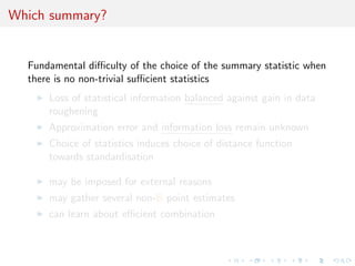
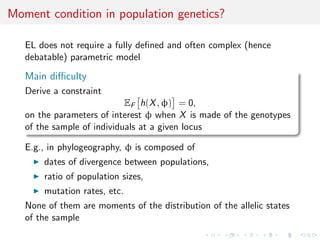
![Summary [about summaries]
Choice of summary statistics is paramount for ABC
validation/performances
At best, ABC approximates π(. | η(y)) [unavoidable]
Model selection feasible with ABC [with caution!]
For estimation, consistency if {θ; µ(θ) = µ0} = θ0 when
Eθ[η(y)] = µ(θ)
For testing consistency if
{µ1(θ1), θ1 ∈ Θ1} ∩ {µ2(θ2), θ2 ∈ Θ2} = ∅
[Marin et al., 2011]](https://image.slidesharecdn.com/i-like-130515231914-phpapp01/85/slides-of-ABC-talk-at-i-like-workshop-Warwick-May-16-95-320.jpg)
![Summary [about summaries]
Choice of summary statistics is paramount for ABC
validation/performances
At best, ABC approximates π(. | η(y)) [unavoidable]
Model selection feasible with ABC [with caution!]
For estimation, consistency if {θ; µ(θ) = µ0} = θ0 when
Eθ[η(y)] = µ(θ)
For testing consistency if
{µ1(θ1), θ1 ∈ Θ1} ∩ {µ2(θ2), θ2 ∈ Θ2} = ∅
[Marin et al., 2011]](https://image.slidesharecdn.com/i-like-130515231914-phpapp01/85/slides-of-ABC-talk-at-i-like-workshop-Warwick-May-16-96-320.jpg)
![Summary [about summaries]
Choice of summary statistics is paramount for ABC
validation/performances
At best, ABC approximates π(. | η(y)) [unavoidable]
Model selection feasible with ABC [with caution!]
For estimation, consistency if {θ; µ(θ) = µ0} = θ0 when
Eθ[η(y)] = µ(θ)
For testing consistency if
{µ1(θ1), θ1 ∈ Θ1} ∩ {µ2(θ2), θ2 ∈ Θ2} = ∅
[Marin et al., 2011]](https://image.slidesharecdn.com/i-like-130515231914-phpapp01/85/slides-of-ABC-talk-at-i-like-workshop-Warwick-May-16-97-320.jpg)
![Summary [about summaries]
Choice of summary statistics is paramount for ABC
validation/performances
At best, ABC approximates π(. | η(y)) [unavoidable]
Model selection feasible with ABC [with caution!]
For estimation, consistency if {θ; µ(θ) = µ0} = θ0 when
Eθ[η(y)] = µ(θ)
For testing consistency if
{µ1(θ1), θ1 ∈ Θ1} ∩ {µ2(θ2), θ2 ∈ Θ2} = ∅
[Marin et al., 2011]](https://image.slidesharecdn.com/i-like-130515231914-phpapp01/85/slides-of-ABC-talk-at-i-like-workshop-Warwick-May-16-98-320.jpg)
![Summary [about summaries]
Choice of summary statistics is paramount for ABC
validation/performances
At best, ABC approximates π(. | η(y)) [unavoidable]
Model selection feasible with ABC [with caution!]
For estimation, consistency if {θ; µ(θ) = µ0} = θ0 when
Eθ[η(y)] = µ(θ)
For testing consistency if
{µ1(θ1), θ1 ∈ Θ1} ∩ {µ2(θ2), θ2 ∈ Θ2} = ∅
[Marin et al., 2011]](https://image.slidesharecdn.com/i-like-130515231914-phpapp01/85/slides-of-ABC-talk-at-i-like-workshop-Warwick-May-16-99-320.jpg)
![Empirical likelihood (EL)
Unavailable likelihoods
ABC methods
ABC as an inference machine
[A]BCel
ABC and EL
Composite likelihood
Illustrations
Conclusion and perspectives](https://image.slidesharecdn.com/i-like-130515231914-phpapp01/85/slides-of-ABC-talk-at-i-like-workshop-Warwick-May-16-100-320.jpg)
![Empirical likelihood (EL)
Dataset x made of n independent replicates x = (x1, . . . , xn) of
some X ∼ F
Generalized moment condition model
EF h(X, φ) = 0,
where h is a known function, and φ an unknown parameter
Corresponding empirical likelihood
Lel(φ|x) = max
p
n
i=1
pi
for all p such that 0 pi 1, i pi = 1, i pi h(xi , φ) = 0.
[Owen, 1988, Bio’ka, & Empirical Likelihood, 2001]](https://image.slidesharecdn.com/i-like-130515231914-phpapp01/85/slides-of-ABC-talk-at-i-like-workshop-Warwick-May-16-101-320.jpg)
![Empirical likelihood (EL)
Dataset x made of n independent replicates x = (x1, . . . , xn) of
some X ∼ F
Generalized moment condition model
EF h(X, φ) = 0,
where h is a known function, and φ an unknown parameter
Corresponding empirical likelihood
Lel(φ|x) = max
p
n
i=1
pi
for all p such that 0 pi 1, i pi = 1, i pi h(xi , φ) = 0.
[Owen, 1988, Bio’ka, & Empirical Likelihood, 2001]](https://image.slidesharecdn.com/i-like-130515231914-phpapp01/85/slides-of-ABC-talk-at-i-like-workshop-Warwick-May-16-102-320.jpg)
![Convergence of EL [3.4]
Theorem 3.4 Let X, Y1, . . . , Yn be independent rv’s with common
distribution F0. For θ ∈ Θ, and the function h(X, θ) ∈ Rs, let
θ0 ∈ Θ be such that
Var(h(Yi , θ0))
is finite and has rank q > 0. If θ0 satisfies
E(h(X, θ0)) = 0,
then
−2 log
Lel(θ0|Y1, . . . , Yn)
n−n
→ χ2
(q)
in distribution when n → ∞.
[Owen, 2001]](https://image.slidesharecdn.com/i-like-130515231914-phpapp01/85/slides-of-ABC-talk-at-i-like-workshop-Warwick-May-16-103-320.jpg)
![Convergence of EL [3.4]
“...The interesting thing about Theorem 3.4 is what is not there. It
includes no conditions to make ^θ a good estimate of θ0, nor even
conditions to ensure a unique value for θ0, nor even that any solution θ0
exists. Theorem 3.4 applies in the just determined, over-determined, and
under-determined cases. When we can prove that our estimating
equations uniquely define θ0, and provide a consistent estimator ^θ of it,
then confidence regions and tests follow almost automatically through
Theorem 3.4.”.
[Owen, 2001]](https://image.slidesharecdn.com/i-like-130515231914-phpapp01/85/slides-of-ABC-talk-at-i-like-workshop-Warwick-May-16-104-320.jpg)
![Raw [A]BCelsampler
Act as if EL was an exact likelihood
[Lazar, 2003]
for i = 1 → N do
generate φi from the prior distribution π(·)
set the weight ωi = Lel(φi |xobs)
end for
return (φi , ωi ), i = 1, . . . , N
Output weighted sample of size N](https://image.slidesharecdn.com/i-like-130515231914-phpapp01/85/slides-of-ABC-talk-at-i-like-workshop-Warwick-May-16-105-320.jpg)
![Raw [A]BCelsampler
Act as if EL was an exact likelihood
[Lazar, 2003]
for i = 1 → N do
generate φi from the prior distribution π(·)
set the weight ωi = Lel(φi |xobs)
end for
return (φi , ωi ), i = 1, . . . , N
Performance evaluated through effective sample size
ESS = 1
N
i=1
ωi
N
j=1
ωj
2](https://image.slidesharecdn.com/i-like-130515231914-phpapp01/85/slides-of-ABC-talk-at-i-like-workshop-Warwick-May-16-106-320.jpg)
![Raw [A]BCelsampler
Act as if EL was an exact likelihood
[Lazar, 2003]
for i = 1 → N do
generate φi from the prior distribution π(·)
set the weight ωi = Lel(φi |xobs)
end for
return (φi , ωi ), i = 1, . . . , N
More advanced algorithms can be adapted to EL:
E.g., adaptive multiple importance sampling (AMIS) of
Cornuet et al. to speed up computations
[Cornuet et al., 2012]](https://image.slidesharecdn.com/i-like-130515231914-phpapp01/85/slides-of-ABC-talk-at-i-like-workshop-Warwick-May-16-107-320.jpg)


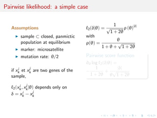

![Example: normal posterior
[A]BCel with two constraints
ESS=155.6
θ
Density
−0.5 0.0 0.5 1.0
0.01.0
ESS=75.93
θ
Density
−0.4 −0.2 0.0 0.2 0.4
0.01.02.0
ESS=76.87
θ
Density
−0.4 −0.2 0.0 0.2
01234
ESS=91.54
θ
Density
−0.6 −0.4 −0.2 0.0 0.2
01234
ESS=108.4
θ
Density
−0.4 0.0 0.2 0.4 0.6
0.01.02.03.0
ESS=85.13
θ
Density
−0.2 0.0 0.2 0.4 0.6
0.01.02.03.0
ESS=149.1
θ
Density
−0.5 0.0 0.5 1.0
0.01.02.0
ESS=96.31
θ
Density
−0.4 0.0 0.2 0.4 0.6
0.01.02.0
ESS=83.77
θ
Density
−0.6 −0.4 −0.2 0.0 0.2 0.401234
ESS=155.7
θ
Density
−0.5 0.0 0.5
0.01.02.0
ESS=92.42
θ
Density
−0.4 0.0 0.2 0.4 0.6
0.01.02.03.0
ESS=95.01
θ
Density
−0.4 0.0 0.2 0.4 0.6
0.01.53.0
ESS=139.2
Density
−0.6 −0.2 0.2 0.6
0.01.02.0
ESS=99.33
Density
−0.4 −0.2 0.0 0.2 0.4
0.01.02.03.0
ESS=87.28
Density
−0.2 0.0 0.2 0.4 0.6
0123
Sample sizes are of 25 (column 1), 50 (column 2) and 75 (column 3)
observations](https://image.slidesharecdn.com/i-like-130515231914-phpapp01/85/slides-of-ABC-talk-at-i-like-workshop-Warwick-May-16-116-320.jpg)
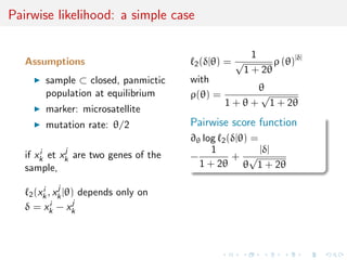
![Example: normal posterior
[A]BCel with three constraints
ESS=300.1
θ
Density
−0.4 0.0 0.4 0.8
0.01.0
ESS=205.5
θ
Density
−0.6 −0.2 0.0 0.2 0.4
0.01.02.0
ESS=179.4
θ
Density
−0.2 0.0 0.2 0.4
0.01.53.0
ESS=265.1
θ
Density
−0.3 −0.2 −0.1 0.0 0.1
01234
ESS=250.3
θ
Density
−0.6 −0.4 −0.2 0.0 0.2
0.01.02.0
ESS=134.8
θ
Density
−0.4 −0.2 0.0 0.1
01234
ESS=331.5
θ
Density
−0.8 −0.4 0.0 0.4
0.01.02.0
ESS=167.4
θ
Density
−0.9 −0.7 −0.5 −0.3
0123
ESS=136.5
θ
Density
−0.4 −0.2 0.0 0.201234
ESS=322.4
θ
Density
−0.2 0.0 0.2 0.4 0.6 0.8
0.01.02.0
ESS=202.7
θ
Density
−0.4 −0.2 0.0 0.2 0.4
0.01.02.03.0
ESS=166
θ
Density
−0.4 −0.2 0.0 0.2
01234
ESS=263.7
Density
−1.0 −0.6 −0.2
0.01.02.0
ESS=190.9
Density
−0.4 −0.2 0.0 0.2 0.4 0.6
0123
ESS=165.3
Density
−0.5 −0.3 −0.1 0.1
0.01.53.0
Sample sizes are of 25 (column 1), 50 (column 2) and 75 (column 3)
observations](https://image.slidesharecdn.com/i-like-130515231914-phpapp01/85/slides-of-ABC-talk-at-i-like-workshop-Warwick-May-16-117-320.jpg)
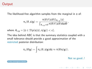
![Example: Superposition of gamma processes
Example of superposition of N renewal processes with waiting
times τij (i = 1, . . . , M, j = 1, . . .) ∼ G(α, β), when N is unknown.
Renewal processes
ζi1 = τi1, ζi2 = ζi1 + τi2, . . .
with observations made of first n values of the ζij ’s,
z1 = min{ζij }, z2 = min{ζij ; ζij > z1}, . . .
ending with
zn = min{ζij ; ζij > zn−1} .
[Cox & Kartsonaki, B’ka, 2012]](https://image.slidesharecdn.com/i-like-130515231914-phpapp01/85/slides-of-ABC-talk-at-i-like-workshop-Warwick-May-16-118-320.jpg)
![Example: Superposition of gamma processes (ABC)
Interesting testing ground for [A]BCel since data (zt) neither iid
nor Markov
Recovery of an iid structure by
1. simulating a pseudo-dataset,
(z1 , . . . , zn ), as in regular
ABC,
2. deriving sequence of
indicators (ν1, . . . , νn), as
z1 = ζν11, z2 = ζν2j2 , . . .
3. exploiting that those
indicators are distributed
from the prior distribution
on the νt’s leading to an iid
sample of G(α, β) variables
Comparison of ABC and
[A]BCel posteriors
α
Density
0 1 2 3 4
0.00.20.40.60.81.01.21.4
β
Density
0 1 2 3 4
0.00.51.01.5
N
Density
0 5 10 15 20
0.000.020.040.060.08
α
Density
0 1 2 3 4
0.00.51.01.5
β
Density
0 1 2 3 4
0.00.20.40.60.81.0
N
Density
0 5 10 15 20
0.000.010.020.030.040.050.06
Top: [A]BCel
Bottom: regular ABC](https://image.slidesharecdn.com/i-like-130515231914-phpapp01/85/slides-of-ABC-talk-at-i-like-workshop-Warwick-May-16-119-320.jpg)
![Example: Superposition of gamma processes (ABC)
Interesting testing ground for [A]BCel since data (zt) neither iid
nor Markov
Recovery of an iid structure by
1. simulating a pseudo-dataset,
(z1 , . . . , zn ), as in regular
ABC,
2. deriving sequence of
indicators (ν1, . . . , νn), as
z1 = ζν11, z2 = ζν2j2 , . . .
3. exploiting that those
indicators are distributed
from the prior distribution
on the νt’s leading to an iid
sample of G(α, β) variables
Comparison of ABC and
[A]BCel posteriors
α
Density
0 1 2 3 4
0.00.20.40.60.81.01.21.4
β
Density
0 1 2 3 4
0.00.51.01.5
N
Density
0 5 10 15 20
0.000.020.040.060.08
α
Density
0 1 2 3 4
0.00.51.01.5
β
Density
0 1 2 3 4
0.00.20.40.60.81.0
N
Density
0 5 10 15 20
0.000.010.020.030.040.050.06
Top: [A]BCel
Bottom: regular ABC](https://image.slidesharecdn.com/i-like-130515231914-phpapp01/85/slides-of-ABC-talk-at-i-like-workshop-Warwick-May-16-120-320.jpg)
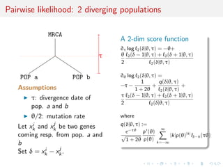
![Pop’gen’: A first experiment
Evolutionary scenario:
MRCA
POP 0 POP 1
τ
Dataset:
50 genes per populations,
100 microsat. loci
Assumptions:
Ne identical over all
populations
φ = (log10 θ, log10 τ)
uniform prior over
(−1., 1.5) × (−1., 1.)
Comparison of the original
ABC with [A]BCel
ESS=7034
log(theta)
Density
0.00 0.05 0.10 0.15 0.20 0.25
051015
log(tau1)
Density
−0.3 −0.2 −0.1 0.0 0.1 0.2 0.3
01234567
histogram = [A]BCel
curve = original ABC
vertical line = “true”
parameter](https://image.slidesharecdn.com/i-like-130515231914-phpapp01/85/slides-of-ABC-talk-at-i-like-workshop-Warwick-May-16-121-320.jpg)
![Pop’gen’: A first experiment
Evolutionary scenario:
MRCA
POP 0 POP 1
τ
Dataset:
50 genes per populations,
100 microsat. loci
Assumptions:
Ne identical over all
populations
φ = (log10 θ, log10 τ)
uniform prior over
(−1., 1.5) × (−1., 1.)
Comparison of the original
ABC with [A]BCel
ESS=7034
log(theta)
Density
0.00 0.05 0.10 0.15 0.20 0.25
051015
log(tau1)
Density
−0.3 −0.2 −0.1 0.0 0.1 0.2 0.3
01234567
histogram = [A]BCel
curve = original ABC
vertical line = “true”
parameter](https://image.slidesharecdn.com/i-like-130515231914-phpapp01/85/slides-of-ABC-talk-at-i-like-workshop-Warwick-May-16-122-320.jpg)
![ABC vs. [A]BCel on 100 replicates of the 1st experiment
Accuracy:
log10 θ log10 τ
ABC [A]BCel ABC [A]BCel
(1) 0.097 0.094 0.315 0.117
(2) 0.071 0.059 0.272 0.077
(3) 0.68 0.81 1.0 0.80
(1) Root Mean Square Error of the posterior mean
(2) Median Absolute Deviation of the posterior median
(3) Coverage of the credibility interval of probability 0.8
Computation time: on a recent 6-core computer
(C++/OpenMP)
ABC ≈ 4 hours
[A]BCel≈ 2 minutes](https://image.slidesharecdn.com/i-like-130515231914-phpapp01/85/slides-of-ABC-talk-at-i-like-workshop-Warwick-May-16-123-320.jpg)
![Pop’gen’: Second experiment
Evolutionary scenario:
MRCA
POP 0 POP 1 POP 2
τ1
τ2
Dataset:
50 genes per populations,
100 microsat. loci
Assumptions:
Ne identical over all
populations
φ =
(log10 θ, log10 τ1, log10 τ2)
non-informative uniform
Comparison of the original ABC
with [A]BCel
histogram = [A]BCel
curve = original ABC
vertical line = “true” parameter](https://image.slidesharecdn.com/i-like-130515231914-phpapp01/85/slides-of-ABC-talk-at-i-like-workshop-Warwick-May-16-124-320.jpg)
![Pop’gen’: Second experiment
Evolutionary scenario:
MRCA
POP 0 POP 1 POP 2
τ1
τ2
Dataset:
50 genes per populations,
100 microsat. loci
Assumptions:
Ne identical over all
populations
φ =
(log10 θ, log10 τ1, log10 τ2)
non-informative uniform
Comparison of the original ABC
with [A]BCel
histogram = [A]BCel
curve = original ABC
vertical line = “true” parameter](https://image.slidesharecdn.com/i-like-130515231914-phpapp01/85/slides-of-ABC-talk-at-i-like-workshop-Warwick-May-16-125-320.jpg)
![Pop’gen’: Second experiment
Evolutionary scenario:
MRCA
POP 0 POP 1 POP 2
τ1
τ2
Dataset:
50 genes per populations,
100 microsat. loci
Assumptions:
Ne identical over all
populations
φ =
(log10 θ, log10 τ1, log10 τ2)
non-informative uniform
Comparison of the original ABC
with [A]BCel
histogram = [A]BCel
curve = original ABC
vertical line = “true” parameter](https://image.slidesharecdn.com/i-like-130515231914-phpapp01/85/slides-of-ABC-talk-at-i-like-workshop-Warwick-May-16-126-320.jpg)
![Pop’gen’: Second experiment
Evolutionary scenario:
MRCA
POP 0 POP 1 POP 2
τ1
τ2
Dataset:
50 genes per populations,
100 microsat. loci
Assumptions:
Ne identical over all
populations
φ =
(log10 θ, log10 τ1, log10 τ2)
non-informative uniform
Comparison of the original ABC
with [A]BCel
histogram = [A]BCel
curve = original ABC
vertical line = “true” parameter](https://image.slidesharecdn.com/i-like-130515231914-phpapp01/85/slides-of-ABC-talk-at-i-like-workshop-Warwick-May-16-127-320.jpg)
![ABC vs. [A]BCel on 100 replicates of the 2nd experiment
Accuracy:
log10 θ log10 τ1 log10 τ2
ABC [A]BCel ABC [A]BCel ABC [A]B
(1) .0059 .0794 .472 .483 29.3 4.7
(2) .048 .053 .32 .28 4.13 3.3
(3) .79 .76 .88 .76 .89 .79
(1) Root Mean Square Error of the posterior mean
(2) Median Absolute Deviation of the posterior median
(3) Coverage of the credibility interval of probability 0.8
Computation time: on a recent 6-core computer
(C++/OpenMP)
ABC ≈ 6 hours
[A]BCel≈ 8 minutes](https://image.slidesharecdn.com/i-like-130515231914-phpapp01/85/slides-of-ABC-talk-at-i-like-workshop-Warwick-May-16-128-320.jpg)
![Comparison
On large datasets, [A]BCel gives more accurate results than ABC
ABC simplifies the dataset through summary statistics
Due to the large dimension of x, the original ABC algorithm
estimates
π θ η(xobs) ,
where η(xobs) is some (non-linear) projection of the observed
dataset on a space with smaller dimension
→ Some information is lost
[A]BCel simplifies the model through a generalized moment
condition model.
→ Here, the moment condition model is based on pairwise
composition likelihood](https://image.slidesharecdn.com/i-like-130515231914-phpapp01/85/slides-of-ABC-talk-at-i-like-workshop-Warwick-May-16-129-320.jpg)
![Conclusion/perspectives
abc part of a wider picture
to handle complex/Big Data
models
many formats of empirical
[likelihood] Bayes methods
available
lack of comparative tools
and of an assessment for
information loss](https://image.slidesharecdn.com/i-like-130515231914-phpapp01/85/slides-of-ABC-talk-at-i-like-workshop-Warwick-May-16-130-320.jpg)

Approximate Bayesian computation (ABC) is a new empirical Bayes method for performing Bayesian inference when the likelihood function is intractable or unavailable in closed form. ABC replaces the likelihood with a non-parametric approximation based on simulating data under different parameter values and comparing simulated and observed data using summary statistics. This allows Bayesian inference to be performed even when direct calculation of the likelihood is not possible. However, ABC introduces an approximation error that is unknown without extensive simulation. Some view ABC as a true Bayesian approach for an estimated or noisy likelihood, while others see it as more of a computational technique that is only approximately Bayesian.
![[A]BCel : a presentation at ABC in Roma](https://cdn.slidesharecdn.com/ss_thumbnails/abcel-130530042650-phpapp02-thumbnail.jpg?width=640&height=640&fit=bounds)


![Introduction to bayesian_networks[1]](https://cdn.slidesharecdn.com/ss_thumbnails/introductiontobayesiannetworks1-150525024327-lva1-app6891-thumbnail.jpg?width=640&height=640&fit=bounds)