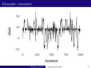
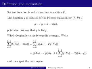
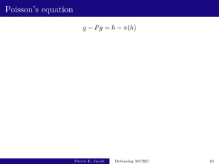
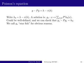
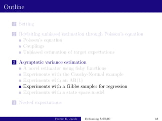
- The document discusses debiasing techniques for Markov chain Monte Carlo (MCMC) algorithms. - It introduces the concept of "fishy functions" which are solutions to Poisson's equation and can be used for control variates to reduce bias and variance in MCMC estimators. - The document outlines different sections including revisiting unbiased estimation through Poisson's equation, asymptotic variance estimation using a novel "fishy function" estimator, and experiments on different examples.

1. Debiasing techniques for
Markov chain Monte Carlo algorithms
Pierre E. Jacob
joint work with
Randal Douc, Anthony Lee, Dootika Vats
Computational methods for unifying multiple statistical analyses
CIRM, October 25, 2022
Pierre E. Jacob Debiasing MCMC 1

2. Outline
1 Setting
2 Revisiting unbiased estimation through Poisson’s equation
Poisson’s equation
Couplings
Unbiased estimation of target expectations
3 Asymptotic variance estimation
A novel estimator using fishy functions
Experiments with the Cauchy-Normal example
Experiments with an AR(1)
Experiments with a Gibbs sampler for regression
Experiments with a state space model
4 Nested expectations
Pierre E. Jacob Debiasing MCMC 2

3. Outline
1 Setting
2 Revisiting unbiased estimation through Poisson’s equation
Poisson’s equation
Couplings
Unbiased estimation of target expectations
3 Asymptotic variance estimation
A novel estimator using fishy functions
Experiments with the Cauchy-Normal example
Experiments with an AR(1)
Experiments with a Gibbs sampler for regression
Experiments with a state space model
4 Nested expectations
Pierre E. Jacob Debiasing MCMC 2

4. Markov chain Monte Carlo
Target probability distribution π.
Example: posterior distribution.
Pierre E. Jacob Debiasing MCMC 3

5. Markov chain Monte Carlo
Target probability distribution π.
Example: posterior distribution.
Test function h, with expectation with respect to π:
π(h) = Eπ[h(X)] =
Z
h(x)π(dx).
Example: h(x) = 1(x > t), π(h) = Pπ(X > t).
Pierre E. Jacob Debiasing MCMC 3

6. Markov chain Monte Carlo
Target probability distribution π.
Example: posterior distribution.
Test function h, with expectation with respect to π:
π(h) = Eπ[h(X)] =
Z
h(x)π(dx).
Example: h(x) = 1(x > t), π(h) = Pπ(X > t).
MCMC: X0 ∼ π0, then Xt|Xt−1 ∼ P(Xt−1, ·) for t ≥ 1.
P is constructed to be π-invariant.
MCMC estimator of π(h): t−1 Pt−1
s=0 h(Xs).
Pierre E. Jacob Debiasing MCMC 3

7. Markov chain Monte Carlo
Target probability distribution π.
Example: posterior distribution.
Test function h, with expectation with respect to π:
π(h) = Eπ[h(X)] =
Z
h(x)π(dx).
Example: h(x) = 1(x > t), π(h) = Pπ(X > t).
MCMC: X0 ∼ π0, then Xt|Xt−1 ∼ P(Xt−1, ·) for t ≥ 1.
P is constructed to be π-invariant.
MCMC estimator of π(h): t−1 Pt−1
s=0 h(Xs).
Pt
(x, ·): distribution of Xt given X0 = x.
πt = π0Pt
: marginal distribution of Xt.
Pt
h(x) = E[h(Xt)|X0 = x]: conditional expectation after t steps.
Pierre E. Jacob Debiasing MCMC 3

8. MCMC convergence and questions
Convergence of marginals (in total variation, Wasserstein, etc):
|πt − π| → 0.
t−1 Pt−1
s=0 h(Xs) is biased for finite t, due to π0 6= π.
Pierre E. Jacob Debiasing MCMC 4

9. MCMC convergence and questions
Convergence of marginals (in total variation, Wasserstein, etc):
|πt − π| → 0.
t−1 Pt−1
s=0 h(Xs) is biased for finite t, due to π0 6= π.
Central limit theorem, for a given test function h:
√
t t−1
t−1
X
s=0
h(Xs) − π(h)
!
→ Normal(0, v(P, h)).
Pierre E. Jacob Debiasing MCMC 4

10. MCMC convergence and questions
Convergence of marginals (in total variation, Wasserstein, etc):
|πt − π| → 0.
t−1 Pt−1
s=0 h(Xs) is biased for finite t, due to π0 6= π.
Central limit theorem, for a given test function h:
√
t t−1
t−1
X
s=0
h(Xs) − π(h)
!
→ Normal(0, v(P, h)).
How to quantify/reduce the bias and the variance?
How to parallelize the computation?
Pierre E. Jacob Debiasing MCMC 4

11. Example: Cauchy-Normal Bayesian inference
Prior θ ∼ Normal(0, σ2), on θ in the model: xi
ind
∼ Cauchy(θ, 1).
Pierre E. Jacob Debiasing MCMC 5

12. Example: Cauchy-Normal Bayesian inference
Prior θ ∼ Normal(0, σ2), on θ in the model: xi
ind
∼ Cauchy(θ, 1).
Posterior:
π(θ|x1, . . . , xn) ∝ exp(−θ2
/2σ2
)
n
Y
i=1
1 + (θ − xi)2
−1
∝ exp(−θ2
/2σ2
)
n
Y
i=1
Z
exp −
1 + (θ − xi)2
2
ηi
!
dηi.
Pierre E. Jacob Debiasing MCMC 5

13. Example: Cauchy-Normal Bayesian inference
Prior θ ∼ Normal(0, σ2), on θ in the model: xi
ind
∼ Cauchy(θ, 1).
Posterior:
π(θ|x1, . . . , xn) ∝ exp(−θ2
/2σ2
)
n
Y
i=1
1 + (θ − xi)2
−1
∝ exp(−θ2
/2σ2
)
n
Y
i=1
Z
exp −
1 + (θ − xi)2
2
ηi
!
dηi.
Gibbs sampler:
ηi|θ ∼ Exponential
1 + (θ − xi)2
2
!
∀i = 1, . . . , n
θ0
|η1, . . . , ηn ∼ Normal
Pn
i=1 ηixi
Pn
i=1 ηi + σ−2
,
1
Pn
i=1 ηi + σ−2
.
Pierre E. Jacob Debiasing MCMC 5

14. Example: target
0.0
0.1
0.2
−20 0 20 40
x
π
(
x
)
Example taken from C. P. Robert, Convergence control methods for
Markov chain Monte Carlo algorithms, 1995.
Pierre E. Jacob Debiasing MCMC 6

15. Example: traceplot
−10
0
10
20
0 250 500 750 1000
iteration
chain
Pierre E. Jacob Debiasing MCMC 7

16. Outline
1 Setting
2 Revisiting unbiased estimation through Poisson’s equation
Poisson’s equation
Couplings
Unbiased estimation of target expectations
3 Asymptotic variance estimation
A novel estimator using fishy functions
Experiments with the Cauchy-Normal example
Experiments with an AR(1)
Experiments with a Gibbs sampler for regression
Experiments with a state space model
4 Nested expectations
Pierre E. Jacob Debiasing MCMC 8

17. Outline
1 Setting
2 Revisiting unbiased estimation through Poisson’s equation
Poisson’s equation
Couplings
Unbiased estimation of target expectations
3 Asymptotic variance estimation
A novel estimator using fishy functions
Experiments with the Cauchy-Normal example
Experiments with an AR(1)
Experiments with a Gibbs sampler for regression
Experiments with a state space model
4 Nested expectations
Pierre E. Jacob Debiasing MCMC 8

18. Outline
1 Setting
2 Revisiting unbiased estimation through Poisson’s equation
Poisson’s equation
Couplings
Unbiased estimation of target expectations
3 Asymptotic variance estimation
A novel estimator using fishy functions
Experiments with the Cauchy-Normal example
Experiments with an AR(1)
Experiments with a Gibbs sampler for regression
Experiments with a state space model
4 Nested expectations
Pierre E. Jacob Debiasing MCMC 8

19. Definition and motivation
Set test function h and π-invariant transition P.
The function g is solution of the Poisson equation for (h, P) if
g − Pg = h − π(h),
pointwise. We say that g is fishy.
Pierre E. Jacob Debiasing MCMC 9

20. Definition and motivation
Set test function h and π-invariant transition P.
The function g is solution of the Poisson equation for (h, P) if
g − Pg = h − π(h),
pointwise. We say that g is fishy.
Why? Originally to study ergodic averages. Write
t−1
X
s=0
(h(Xs) − π(h)) =
t−1
X
s=0
(g(Xs) − Pg(Xs))
= g(X0) − Pg(Xt−1) +
t−1
X
s=1
(g(Xs) − Pg(Xs−1)),
and then spot the martingale.
Pierre E. Jacob Debiasing MCMC 9

21. Poisson’s equation
g − Pg = h − π(h)
Pierre E. Jacob Debiasing MCMC 10

22. Poisson’s equation
g − Pg = h − π(h)
Write h0 = h − π(h). A solution is: g? : x 7→
P
t≥0 Pth0(x).
Could be well-defined, and we can check that g? − Pg? = h0.
We call g? “star fish” for obvious reasons.
Pierre E. Jacob Debiasing MCMC 10

23. Poisson’s equation
g − Pg = h − π(h)
Write h0 = h − π(h). A solution is: g? : x 7→
P
t≥0 Pth0(x).
Could be well-defined, and we can check that g? − Pg? = h0.
We call g? “star fish” for obvious reasons.
Note that if g is fishy, then g + constant is also fishy.
Pierre E. Jacob Debiasing MCMC 10

24. Poisson’s equation
g − Pg = h − π(h)
Write h0 = h − π(h). A solution is: g? : x 7→
P
t≥0 Pth0(x).
Could be well-defined, and we can check that g? − Pg? = h0.
We call g? “star fish” for obvious reasons.
Note that if g is fishy, then g + constant is also fishy.
If g? ∈ L1(π), then all fishy functions are equal up to an
additive constant, and g? is the one such that π(g?) = 0.
Pierre E. Jacob Debiasing MCMC 10

25. Poisson’s equation
g − Pg = h − π(h)
Write h0 = h − π(h). A solution is: g? : x 7→
P
t≥0 Pth0(x).
Could be well-defined, and we can check that g? − Pg? = h0.
We call g? “star fish” for obvious reasons.
Note that if g is fishy, then g + constant is also fishy.
If g? ∈ L1(π), then all fishy functions are equal up to an
additive constant, and g? is the one such that π(g?) = 0.
Another fishy function, where y is fixed,
gy : x 7→ g?(x) − g?(y) =
X
t≥0
{Pt
h(x) − Pt
h(y)}.
We call gy “friendly fish” because it is our friend.
Pierre E. Jacob Debiasing MCMC 10

26. Fishy functions and Monte Carlo
Fishy functions arise for various reasons in Monte Carlo.
Asymptotic bias: g?(x) =
P
t≥0 Pth0(x) is the asymptotic bias
of MCMC, initialized at x:
g?(x) = lim
t→∞
t
(
Ex
t−1
t−1
X
s=0
h(Xs)
#
− π(h)
)
.
Kontoyiannis Dellaportas, Notes on using control variates for
estimation with reversible MCMC samplers, 2009.
Pierre E. Jacob Debiasing MCMC 11

27. Fishy functions and Monte Carlo
Control variates: replace
t−1
t−1
X
s=0
h(Xs) by t−1
t−1
X
s=0
{h(Xs) − (g(Xs) − Pg(Xs))}.
At stationarity, expectation is unchanged: π(g − Pg) = 0.
Variance is reduced to zero if g is fishy: h − (g − Pg) = π(h).
Andradóttir, Heyman, Ott, Variance reduction through smoothing
and control variates for Markov chain simulations, 1993.
Pierre E. Jacob Debiasing MCMC 12

28. Outline
1 Setting
2 Revisiting unbiased estimation through Poisson’s equation
Poisson’s equation
Couplings
Unbiased estimation of target expectations
3 Asymptotic variance estimation
A novel estimator using fishy functions
Experiments with the Cauchy-Normal example
Experiments with an AR(1)
Experiments with a Gibbs sampler for regression
Experiments with a state space model
4 Nested expectations
Pierre E. Jacob Debiasing MCMC 12

29. Pairs of chains that meet
Generate two chains (Xt) and (Yt) as follows:
set X0 = x and Y0 = y.
for t ≥ 1, sample (Xt, Yt)|(Xt−1, Yt−1) ∼ P̄ ((Xt−1, Yt−1), ·).
Pierre E. Jacob Debiasing MCMC 13

30. Pairs of chains that meet
Generate two chains (Xt) and (Yt) as follows:
set X0 = x and Y0 = y.
for t ≥ 1, sample (Xt, Yt)|(Xt−1, Yt−1) ∼ P̄ ((Xt−1, Yt−1), ·).
Here P̄ is a coupling of P with itself:
P̄((x, y), A×X) = P(x, A), P̄((x, y), X×A) = P(y, A), A ∈ X.
Pierre E. Jacob Debiasing MCMC 13

31. Pairs of chains that meet
Generate two chains (Xt) and (Yt) as follows:
set X0 = x and Y0 = y.
for t ≥ 1, sample (Xt, Yt)|(Xt−1, Yt−1) ∼ P̄ ((Xt−1, Yt−1), ·).
Here P̄ is a coupling of P with itself:
P̄((x, y), A×X) = P(x, A), P̄((x, y), X×A) = P(y, A), A ∈ X.
And P̄ is faithful: P̄((x, x), {(x0, y0) : x0 = y0}) = 1 for all x ∈ X.
Pierre E. Jacob Debiasing MCMC 13

32. Pairs of chains that meet
Generate two chains (Xt) and (Yt) as follows:
set X0 = x and Y0 = y.
for t ≥ 1, sample (Xt, Yt)|(Xt−1, Yt−1) ∼ P̄ ((Xt−1, Yt−1), ·).
Here P̄ is a coupling of P with itself:
P̄((x, y), A×X) = P(x, A), P̄((x, y), X×A) = P(y, A), A ∈ X.
And P̄ is faithful: P̄((x, x), {(x0, y0) : x0 = y0}) = 1 for all x ∈ X.
Denote by τ the “meeting time” such that Xt = Yt for t ≥ τ.
For an arbitrary P̄, τ could be infinite, but we can often
construct P̄ such that τ is finite (somewhat surprisingly).
Pierre E. Jacob Debiasing MCMC 13

33. Example: coupled kernel
Recall our Gibbs sampler:
ηi|θ ∼ Exponential
1 + (θ − xi)2
2
!
∀i = 1, . . . , n
θ0
|η1, . . . , ηn ∼ Normal
Pn
i=1 ηixi
Pn
i=1 ηi + σ−2
,
1
Pn
i=1 ηi + σ−2
.
Pierre E. Jacob Debiasing MCMC 14

34. Example: coupled kernel
Recall our Gibbs sampler:
ηi|θ ∼ Exponential
1 + (θ − xi)2
2
!
∀i = 1, . . . , n
θ0
|η1, . . . , ηn ∼ Normal
Pn
i=1 ηixi
Pn
i=1 ηi + σ−2
,
1
Pn
i=1 ηi + σ−2
.
Start from θ(1), θ(2) that are possibly unequal.
Pierre E. Jacob Debiasing MCMC 14

35. Example: coupled kernel
Recall our Gibbs sampler:
ηi|θ ∼ Exponential
1 + (θ − xi)2
2
!
∀i = 1, . . . , n
θ0
|η1, . . . , ηn ∼ Normal
Pn
i=1 ηixi
Pn
i=1 ηi + σ−2
,
1
Pn
i=1 ηi + σ−2
.
Start from θ(1), θ(2) that are possibly unequal.
Generate η(1), η(2) using common uniforms:
∀j = 1, 2 ∀i = 1, . . . , n η
(j)
i = −
1 + (θ(j) − xi)2
2
!−1
log Ui.
Pierre E. Jacob Debiasing MCMC 14

36. Example: coupled kernel
Recall our Gibbs sampler:
ηi|θ ∼ Exponential
1 + (θ − xi)2
2
!
∀i = 1, . . . , n
θ0
|η1, . . . , ηn ∼ Normal
Pn
i=1 ηixi
Pn
i=1 ηi + σ−2
,
1
Pn
i=1 ηi + σ−2
.
Start from θ(1), θ(2) that are possibly unequal.
Generate η(1), η(2) using common uniforms:
∀j = 1, 2 ∀i = 1, . . . , n η
(j)
i = −
1 + (θ(j) − xi)2
2
!−1
log Ui.
Sample θ0(1), θ0(2), such that P(θ0(1) = θ0(2)|η(1), η(2)) is maximal.
Pierre E. Jacob Debiasing MCMC 14

37. A maximal coupling of two Normals
0.0
0.2
0.4
0.6
0.8
−5 0 5
density
−5
0
5
0.00
0.05
0.10
0.15
0.20
density
y
−5
0
5
−5 0 5
x
Pierre E. Jacob Debiasing MCMC 15

38. A maximal coupling of two tractable distributions
Input: p and q.
Output: (X, Y ) where X ∼ p, Y ∼ q and P(X = Y ) is maximal.
Note: max P(X = Y ) = 1 − |p − q|TV.
1 Sample X ∼ p and W ∼ Uniform(0, 1).
2 If W ≤ q(X)/p(X), set Y = X.
3 Otherwise, sample Y ? ∼ q and W? ∼ Uniform(0, 1)
until W? p(Y ?)/q(Y ?), then set Y = Y ?.
e.g. Thorisson, Coupling, stationarity, and regeneration, 2000,
Chapter 1, Section 4.5.
Pierre E. Jacob Debiasing MCMC 16

39. Example: coupled trajectories that meet
−10
0
10
20
0 100 200 300 400 500
iteration
coupled
chains
Pierre E. Jacob Debiasing MCMC 17

40. Couplings in realistic MCMC settings
Faithful couplings, generating exact meetings, have been
designed in many settings. Algorithm-specific.
Xu, Fjelde, Sutton, Ge, Couplings for Multinomial
Hamiltonian Monte Carlo, 2021
Ruiz, Titsias, Cemgil Doucet, Unbiased gradient estimation for
variational auto-encoders using coupled Markov chains, 2021.
Trippe, Nguyen Broderick, Many processors, little time:
MCMC for partitions via optimal transport couplings, 2022.
Kelly, Ryder Clarté, Lagged couplings diagnose Markov chain
Monte Carlo phylogenetic inference, 2022.
Pierre E. Jacob Debiasing MCMC 18

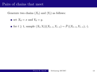
41. Assumption on meeting time
Main assumption. For some κ 1, Eπ⊗π[τκ] ∞.
Equivalent to P(τ t) being smaller than t−κ as t → ∞.
Holds for all κ 1 if tails are Geometric.
Pierre E. Jacob Debiasing MCMC 19

42. CLT for Markov chain averages
Let h ∈ Lm(π) for some m 2κ/(κ − 1).
Then
g? ∈ L1(π),
h0 · g? ∈ L1(π),
the CLT holds for π-almost all X0 with
v(P, h) = 2π(h0 · g?) − π(h2
0) ∞.
Pierre E. Jacob Debiasing MCMC 20

43. Example: verifying the assumption
ηi|θ ∼ Exponential
1 + (θ − xi)2
2
!
∀i = 1, . . . , n
θ0
|η1, . . . , ηn ∼ Normal
Pn
i=1 ηixi
Pn
i=1 ηi + σ−2
,
1
Pn
i=1 ηi + σ−2
.
Pierre E. Jacob Debiasing MCMC 21

44. Example: verifying the assumption
ηi|θ ∼ Exponential
1 + (θ − xi)2
2
!
∀i = 1, . . . , n
θ0
|η1, . . . , ηn ∼ Normal
Pn
i=1 ηixi
Pn
i=1 ηi + σ−2
,
1
Pn
i=1 ηi + σ−2
.
For θ(1) 6= θ(2), consider next draws.
Pierre E. Jacob Debiasing MCMC 21

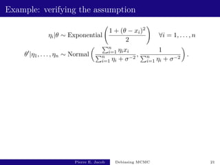
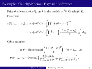
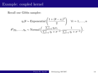
45. Example: verifying the assumption
ηi|θ ∼ Exponential
1 + (θ − xi)2
2
!
∀i = 1, . . . , n
θ0
|η1, . . . , ηn ∼ Normal
Pn
i=1 ηixi
Pn
i=1 ηi + σ−2
,
1
Pn
i=1 ηi + σ−2
.
For θ(1) 6= θ(2), consider next draws.
Means of Normals are always in [− max |xi|, + max |xi|].
Pierre E. Jacob Debiasing MCMC 21

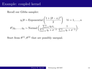
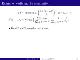
46. Example: verifying the assumption
ηi|θ ∼ Exponential
1 + (θ − xi)2
2
!
∀i = 1, . . . , n
θ0
|η1, . . . , ηn ∼ Normal
Pn
i=1 ηixi
Pn
i=1 ηi + σ−2
,
1
Pn
i=1 ηi + σ−2
.
For θ(1) 6= θ(2), consider next draws.
Means of Normals are always in [− max |xi|, + max |xi|].
0 ≤ ηi ≤ −2 log Ui almost surely for both chains.
Pierre E. Jacob Debiasing MCMC 21

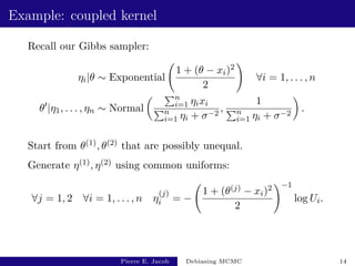
47. Example: verifying the assumption
ηi|θ ∼ Exponential
1 + (θ − xi)2
2
!
∀i = 1, . . . , n
θ0
|η1, . . . , ηn ∼ Normal
Pn
i=1 ηixi
Pn
i=1 ηi + σ−2
,
1
Pn
i=1 ηi + σ−2
.
For θ(1) 6= θ(2), consider next draws.
Means of Normals are always in [− max |xi|, + max |xi|].
0 ≤ ηi ≤ −2 log Ui almost surely for both chains.
Variances of Normals simultaneously within (c, d) ⊂ (0, ∞)
with probability ≥ quantity independent of θ(1), θ(2).
Pierre E. Jacob Debiasing MCMC 21

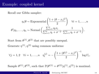
48. Example: verifying the assumption
ηi|θ ∼ Exponential
1 + (θ − xi)2
2
!
∀i = 1, . . . , n
θ0
|η1, . . . , ηn ∼ Normal
Pn
i=1 ηixi
Pn
i=1 ηi + σ−2
,
1
Pn
i=1 ηi + σ−2
.
For θ(1) 6= θ(2), consider next draws.
Means of Normals are always in [− max |xi|, + max |xi|].
0 ≤ ηi ≤ −2 log Ui almost surely for both chains.
Variances of Normals simultaneously within (c, d) ⊂ (0, ∞)
with probability ≥ quantity independent of θ(1), θ(2).
TV between such Normals ≤ 1 − with 0.
Pierre E. Jacob Debiasing MCMC 21

49. Example: verifying the assumption
ηi|θ ∼ Exponential
1 + (θ − xi)2
2
!
∀i = 1, . . . , n
θ0
|η1, . . . , ηn ∼ Normal
Pn
i=1 ηixi
Pn
i=1 ηi + σ−2
,
1
Pn
i=1 ηi + σ−2
.
For θ(1) 6= θ(2), consider next draws.
Means of Normals are always in [− max |xi|, + max |xi|].
0 ≤ ηi ≤ −2 log Ui almost surely for both chains.
Variances of Normals simultaneously within (c, d) ⊂ (0, ∞)
with probability ≥ quantity independent of θ(1), θ(2).
TV between such Normals ≤ 1 − with 0.
Assumption satisfied for all κ 1.
Pierre E. Jacob Debiasing MCMC 21

50. Estimation of fishy function evaluations
Friendly fish gy : x 7→ g?(x) − g?(y) =
P
t≥0{Pth(x) − Pth(y)}.
Pierre E. Jacob Debiasing MCMC 22

51. Estimation of fishy function evaluations
Friendly fish gy : x 7→ g?(x) − g?(y) =
P
t≥0{Pth(x) − Pth(y)}.
Define the following estimator:
Gy(x) :=
τ−1
X
t=0
{h(Xt) − h(Yt)},
where X0 = x, and Y0 = y, τ = inf{t ≥ 1 : Xt = Yt}.
Can be implemented, requires τ simulations from P̄.
Pierre E. Jacob Debiasing MCMC 22

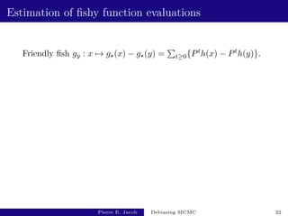
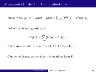
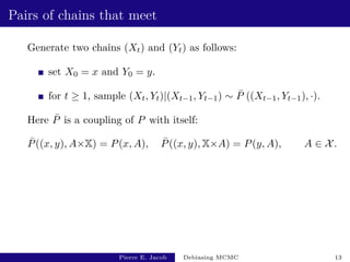
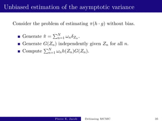
52. Estimation of fishy function evaluations
friendly fish evaluation: gy(x) =
∞
X
t=0
{Pt
h(x) − Pt
h(y)}
its estimator: Gy(x) =
∞
X
t=0
{h(Xt) − h(Yt)}
Let h ∈ Lm(π) for some m κ/(κ − 1).
For π ⊗ π-almost all (x, y), E [Gy(x)] = gy(x),
and for p ≥ 1 such that 1
p 1
m + 1
κ , E [|Gy(x)|p
] ∞.
Pierre E. Jacob Debiasing MCMC 23

53. Example: fishy function for h : x 7→ x
−100
0
100
−20 0 20 40
x
fishy
function(x)
Pierre E. Jacob Debiasing MCMC 24

54. Outline
1 Setting
2 Revisiting unbiased estimation through Poisson’s equation
Poisson’s equation
Couplings
Unbiased estimation of target expectations
3 Asymptotic variance estimation
A novel estimator using fishy functions
Experiments with the Cauchy-Normal example
Experiments with an AR(1)
Experiments with a Gibbs sampler for regression
Experiments with a state space model
4 Nested expectations
Pierre E. Jacob Debiasing MCMC 24

55. Poisson equation → unbiased estimation
Let’s start again from the Poisson equation:
g − Pg = h − π(h),
and re-arrange:
π(h) = h(x) + Pg(x) − g(x) ∀x ∈ X.
Setting x ∈ X arbitrarily, we can estimate the right-hand side.
Pierre E. Jacob Debiasing MCMC 25

56. Poisson equation → unbiased estimation
Let’s start again from the Poisson equation:
g − Pg = h − π(h),
and re-arrange:
π(h) = h(x) + Pg(x) − g(x) ∀x ∈ X.
Setting x ∈ X arbitrarily, we can estimate the right-hand side.
Pg?(x) − g?(x) can be estimated using coupled chains.
Pierre E. Jacob Debiasing MCMC 25

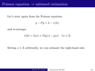
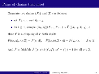
57. Poisson equation → unbiased estimation
For any x ∈ X, let X1 ∼ P(x, ·), and let Gy(x0) be an unbiased
estimator of gy(x0), for π-almost any x0, y.
Then
Ex[Gx(X1)] = Ex[g?(X1) − g?(x)]
= Pg?(x) − g?(x).
Thus Gx(X1) is an unbiased estimator of π(h) − h(x).
Pierre E. Jacob Debiasing MCMC 26

58. Poisson equation → unbiased estimation
For any x ∈ X, let X1 ∼ P(x, ·), and let Gy(x0) be an unbiased
estimator of gy(x0), for π-almost any x0, y.
Then
Ex[Gx(X1)] = Ex[g?(X1) − g?(x)]
= Pg?(x) − g?(x).
Thus Gx(X1) is an unbiased estimator of π(h) − h(x).
We can randomize x: X0
0 ∼ π0, Y 0
0 ∼ π0, and X0
1 ∼ P(X0
0, ·),
E[GY 0
0
(X0
1)] = π(h) − π0(h).
Glynn Rhee, Exact Estimation for Markov Chain Equilibrium
Expectations, 2014.
Pierre E. Jacob Debiasing MCMC 26

59. Poisson equation → unbiased estimation
For starting index k, we can draw X0
k ∼ πk, Y 0
k ∼ πk, then
X0
k+1 ∼ P(X0
k, ·), then h(X0
k) + GY 0
k
(X0
k+1) is unbiased for π(h).
Pierre E. Jacob Debiasing MCMC 27

60. Poisson equation → unbiased estimation
For starting index k, we can draw X0
k ∼ πk, Y 0
k ∼ πk, then
X0
k+1 ∼ P(X0
k, ·), then h(X0
k) + GY 0
k
(X0
k+1) is unbiased for π(h).
Dropping primes, replacing P by PL with L ∈ N, and averaging
estimators obtained for starting indices k, . . . , `,
H
(L)
k:` =
1
` − k + 1
`
X
t=k
h(Xt)
+
1
` − k + 1
`
X
s=k
∞
X
j=1
{h(Xs+jL) − h(Ys+(j−1)L)},
where Xt+L = Yt for t ≥ τ. Unbiased for π(h).
Jacob, O’Leary Atchadé, Unbiased Markov chain Monte Carlo with
couplings, 2020 + discussion by Vanetti Doucet.
Pierre E. Jacob Debiasing MCMC 27

61. Results
Estimator H
(L)
k:` , pronounced “H
(L)
k:` ” (in French “
(L)
k:` ”).
Tuning parameters: “burn-in” k, length `, lag L.
H
(L)
k:` = standard MCMC estimator + bias correction term.
Pierre E. Jacob Debiasing MCMC 28

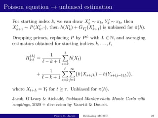
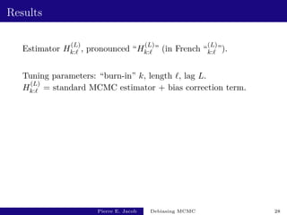
62. Results
Estimator H
(L)
k:` , pronounced “H
(L)
k:` ” (in French “
(L)
k:` ”).
Tuning parameters: “burn-in” k, length `, lag L.
H
(L)
k:` = standard MCMC estimator + bias correction term.
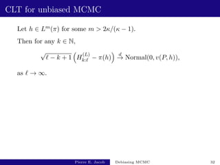
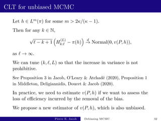
Let h ∈ Lm(π) for some m κ/(κ − 1), and dπ0/dπ ≤ M.
Then for any k, ` ∈ N with ` ≥ k, E[H
(L)
k:` ] = π(h),
and for p ≥ 1 such that 1
p 1
m + 1
κ , E[|H
(L)
k:` |p]
1
p ∞.
Pierre E. Jacob Debiasing MCMC 28

63. Signed measure estimator
Replacing function evaluations by delta masses leads to
π̂(dx) =
1
` − k + 1
`
X
t=k
δXt (dx) +
τ(L)−1
X
t=k+L
vt
` − k + 1
δXt − δYt−L
(dx)
with
vt = b(t − k)/Lc − dmax(L, t − `)/Le + 1.
Pierre E. Jacob Debiasing MCMC 29

64. Signed measure estimator
Replacing function evaluations by delta masses leads to
π̂(dx) =
1
` − k + 1
`
X
t=k
δXt (dx) +
τ(L)−1
X
t=k+L
vt
` − k + 1
δXt − δYt−L
(dx)
with
vt = b(t − k)/Lc − dmax(L, t − `)/Le + 1.
We can just write
π̂(dx) =
N
X
n=1
ωnδZn (dx),
where
PN
n=1 ωn = 1 but some ωn might be negative.
Pierre E. Jacob Debiasing MCMC 29

65. Upper bounds using couplings
Introducing πt+jL with j ≥ 1 between πt and π = π∞,
applying triangle inequalities, using the coupling representation
of TV, and interchanging infinite sum and expectation,
|πt − π|TV ≤ E
τ − L − t
L
.
Biswas, Jacob Vanetti, Estimating Convergence of Markov chains
with L-Lag Couplings, 2019.
Craiu Meng, Double happiness: Enhancing the coupled gains of
L-lag coupling via control variates, 2020.
Pierre E. Jacob Debiasing MCMC 30

66. Example: TV upper bounds
1e−04
1e−03
1e−02
1e−01
1e+00
0 50 100 150
iteration
TV
distance
Pierre E. Jacob Debiasing MCMC 31

67. CLT for unbiased MCMC
Let h ∈ Lm(π) for some m 2κ/(κ − 1).
Then for any k ∈ N,
√
` − k + 1
H
(L)
k:` − π(h)
d
→ Normal(0, v(P, h)),
as ` → ∞.
Pierre E. Jacob Debiasing MCMC 32

68. CLT for unbiased MCMC
Let h ∈ Lm(π) for some m 2κ/(κ − 1).
Then for any k ∈ N,
√
` − k + 1
H
(L)
k:` − π(h)
d
→ Normal(0, v(P, h)),
as ` → ∞.
We can tune (k, `, L) so that the increase in variance is not
prohibitive.
See Proposition 3 in Jacob, O’Leary Atchadé (2020), Proposition 1
in Middleton, Deligiannidis, Doucet Jacob (2020).
Pierre E. Jacob Debiasing MCMC 32

69. CLT for unbiased MCMC
Let h ∈ Lm(π) for some m 2κ/(κ − 1).
Then for any k ∈ N,
√
` − k + 1
H
(L)
k:` − π(h)
d
→ Normal(0, v(P, h)),
as ` → ∞.
We can tune (k, `, L) so that the increase in variance is not
prohibitive.
See Proposition 3 in Jacob, O’Leary Atchadé (2020), Proposition 1
in Middleton, Deligiannidis, Doucet Jacob (2020).
In practice, we need to estimate v(P, h) if we want to assess the
loss of efficiency incurred by the removal of the bias.
Pierre E. Jacob Debiasing MCMC 32

70. CLT for unbiased MCMC
Let h ∈ Lm(π) for some m 2κ/(κ − 1).
Then for any k ∈ N,
√
` − k + 1
H
(L)
k:` − π(h)
d
→ Normal(0, v(P, h)),
as ` → ∞.
We can tune (k, `, L) so that the increase in variance is not
prohibitive.
See Proposition 3 in Jacob, O’Leary Atchadé (2020), Proposition 1
in Middleton, Deligiannidis, Doucet Jacob (2020).
In practice, we need to estimate v(P, h) if we want to assess the
loss of efficiency incurred by the removal of the bias.
We propose a new estimator of v(P, h), which is also unbiased.
Pierre E. Jacob Debiasing MCMC 32

71. Outline
1 Setting
2 Revisiting unbiased estimation through Poisson’s equation
Poisson’s equation
Couplings
Unbiased estimation of target expectations
3 Asymptotic variance estimation
A novel estimator using fishy functions
Experiments with the Cauchy-Normal example
Experiments with an AR(1)
Experiments with a Gibbs sampler for regression
Experiments with a state space model
4 Nested expectations
Pierre E. Jacob Debiasing MCMC 32

72. Outline
1 Setting
2 Revisiting unbiased estimation through Poisson’s equation
Poisson’s equation
Couplings
Unbiased estimation of target expectations
3 Asymptotic variance estimation
A novel estimator using fishy functions
Experiments with the Cauchy-Normal example
Experiments with an AR(1)
Experiments with a Gibbs sampler for regression
Experiments with a state space model
4 Nested expectations
Pierre E. Jacob Debiasing MCMC 32

73. Central limit theorem
Markov kernel P, target π, test function h,
√
t t−1
t−1
X
s=0
h(Xs) − π(h)
!
→ Normal(0, v(P, h)),
where v(P, h) is the asymptotic variance.
Pierre E. Jacob Debiasing MCMC 33

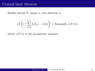
74. Central limit theorem
Markov kernel P, target π, test function h,
√
t t−1
t−1
X
s=0
h(Xs) − π(h)
!
→ Normal(0, v(P, h)),
where v(P, h) is the asymptotic variance.
The limit of V[t−1/2 Pt−1
s=0 h(Xs)] as t → ∞ is
v(P, h) = V(h(X0)) + 2
∞
X
t=1
Cov(h(X0), h(Xt)).
Estimate v(P, h): well-known problem but still difficult.
Spectral variance, batch means, initial sequence. . .
Pierre E. Jacob Debiasing MCMC 33

75. Central limit theorem
Using the Poisson equation to establish a CLT for Markov chain
ergodic averages, leads to the following equivalent expression
v(P, h) = Eπ[{g(X1) − Pg(X0)}2
].
Pierre E. Jacob Debiasing MCMC 34

76. Central limit theorem
Using the Poisson equation to establish a CLT for Markov chain
ergodic averages, leads to the following equivalent expression
v(P, h) = Eπ[{g(X1) − Pg(X0)}2
].
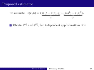
By simple manipulations, using h − π(h) = g − Pg, we can write
v(P, h) = 2π({h − π(h)}g) − (π(h2
) − π(h)2
).
Pierre E. Jacob Debiasing MCMC 34

77. Central limit theorem
Using the Poisson equation to establish a CLT for Markov chain
ergodic averages, leads to the following equivalent expression
v(P, h) = Eπ[{g(X1) − Pg(X0)}2
].
By simple manipulations, using h − π(h) = g − Pg, we can write
v(P, h) = 2π({h − π(h)}g) − (π(h2
) − π(h)2
).
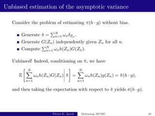
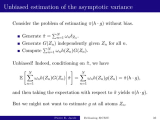
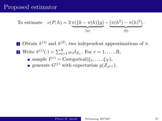
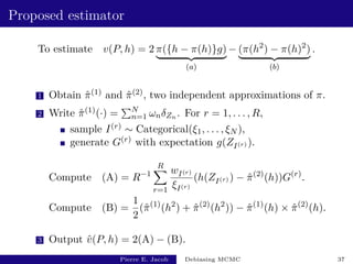
We can obtain unbiased approximations π̂ =
PN
n=1 ωnδZn of π,
and we can estimate g unbiasedly with G, point-wise.
Pierre E. Jacob Debiasing MCMC 34

78. Unbiased estimation of the asymptotic variance
Consider the problem of estimating π(h · g) without bias.
Generate π̂ =
PN
n=1 ωnδZn .
Generate G(Zn) independently given Zn for all n.
Compute
PN
n=1 ωnh(Zn)G(Zn).
Pierre E. Jacob Debiasing MCMC 35

79. Unbiased estimation of the asymptotic variance
Consider the problem of estimating π(h · g) without bias.
Generate π̂ =
PN
n=1 ωnδZn .
Generate G(Zn) independently given Zn for all n.
Compute
PN
n=1 ωnh(Zn)G(Zn).
Unbiased! Indeed, conditioning on π̂, we have
E
N
X
n=1
ωnh(Zn)G(Zn) π̂
#
=
N
X
n=1
ωnh(Zn)g(Zn) = π̂(h · g),
and then taking the expectation with respect to π̂ yields π(h · g).
Pierre E. Jacob Debiasing MCMC 35

80. Unbiased estimation of the asymptotic variance
Consider the problem of estimating π(h · g) without bias.
Generate π̂ =
PN
n=1 ωnδZn .
Generate G(Zn) independently given Zn for all n.
Compute
PN
n=1 ωnh(Zn)G(Zn).
Unbiased! Indeed, conditioning on π̂, we have
E
N
X
n=1
ωnh(Zn)G(Zn) π̂
#
=
N
X
n=1
ωnh(Zn)g(Zn) = π̂(h · g),
and then taking the expectation with respect to π̂ yields π(h · g).
But we might not want to estimate g at all atoms Zn.
Pierre E. Jacob Debiasing MCMC 35

81. Unbiased estimation of the asymptotic variance
We can sample an index I ∈ {1, . . . , N}, according to some
probabilities (ξ1, . . . , ξN ), and estimate g only at atom ZI.
Pierre E. Jacob Debiasing MCMC 36

82. Unbiased estimation of the asymptotic variance
We can sample an index I ∈ {1, . . . , N}, according to some
probabilities (ξ1, . . . , ξN ), and estimate g only at atom ZI.
Then ωI
ξI
h(ZI)G(ZI) is an unbiased estimator of π(h · g).
Pierre E. Jacob Debiasing MCMC 36

83. Unbiased estimation of the asymptotic variance
We can sample an index I ∈ {1, . . . , N}, according to some
probabilities (ξ1, . . . , ξN ), and estimate g only at atom ZI.
Then ωI
ξI
h(ZI)G(ZI) is an unbiased estimator of π(h · g).
We can sample R indices, and balance the cost of sampling π̂
with the cost of estimating g at R locations.
If ξ1 = . . . = ξN = N−1, we can use reservoir sampling to sample
the indices, so that the memory cost is ∝ R instead of ∝ N.
Pierre E. Jacob Debiasing MCMC 36

84. Proposed estimator
To estimate v(P, h) = 2 π({h − π(h)}g)
| {z }
(a)
− (π(h2
) − π(h)2
)
| {z }
(b)
.
1 Obtain π̂(1) and π̂(2), two independent approximations of π.
Pierre E. Jacob Debiasing MCMC 37

85. Proposed estimator
To estimate v(P, h) = 2 π({h − π(h)}g)
| {z }
(a)
− (π(h2
) − π(h)2
)
| {z }
(b)
.
1 Obtain π̂(1) and π̂(2), two independent approximations of π.
2 Write π̂(1)(·) =
PN
n=1 ωnδZn . For r = 1, . . . , R,
sample I(r) ∼ Categorical(ξ1, . . . , ξN ),
generate G(r) with expectation g(ZI(r) ).
Pierre E. Jacob Debiasing MCMC 37

86. Proposed estimator
To estimate v(P, h) = 2 π({h − π(h)}g)
| {z }
(a)
− (π(h2
) − π(h)2
)
| {z }
(b)
.
1 Obtain π̂(1) and π̂(2), two independent approximations of π.
2 Write π̂(1)(·) =
PN
n=1 ωnδZn . For r = 1, . . . , R,
sample I(r) ∼ Categorical(ξ1, . . . , ξN ),
generate G(r) with expectation g(ZI(r) ).
Compute (A) = R−1
R
X
r=1
wI(r)
ξI(r)
(h(ZI(r) ) − π̂(2)
(h))G(r)
.
Compute (B) =
1
2
(π̂(1)
(h2
) + π̂(2)
(h2
)) − π̂(1)
(h) × π̂(2)
(h).
3 Output v̂(P, h) = 2(A) − (B).
Pierre E. Jacob Debiasing MCMC 37

87. Results
Let h ∈ Lm(π) for some m 2κ/(κ − 2).
Assume ξk = 1/N for k ∈ {1, . . . , N}.
Then for any R ≥ 1 and π-almost all y, E [v̂(P, h)] = v(P, h),
and for p ≥ 1 such that 1
p 2
m + 2
κ , E [|v̂(P, h)|p
] ∞.
Pierre E. Jacob Debiasing MCMC 38

88. Tuning
Choice of R, the number of fishy estimates.
Default: try to balance the costs of (G(r))R
r=1 and π̂.
Choice of ξ, selection probabilities.
Default: 1/N. Enables reservoir sampling.
Choice of y in the definition of gy : x 7→ g?(x) − g?(y).
Default: y ∼ π0, so Gy estimates x 7→ g?(x) − π0(g?).
Pierre E. Jacob Debiasing MCMC 39

89. Outline
1 Setting
2 Revisiting unbiased estimation through Poisson’s equation
Poisson’s equation
Couplings
Unbiased estimation of target expectations
3 Asymptotic variance estimation
A novel estimator using fishy functions
Experiments with the Cauchy-Normal example
Experiments with an AR(1)
Experiments with a Gibbs sampler for regression
Experiments with a state space model
4 Nested expectations
Pierre E. Jacob Debiasing MCMC 39

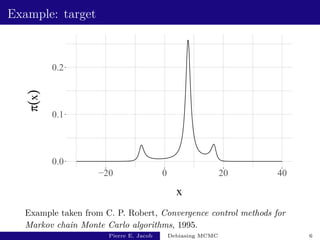
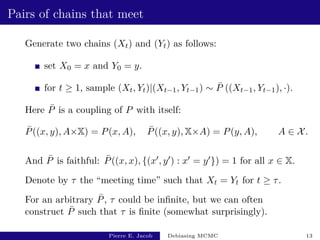
90. Cauchy-Normal: performance
Gibbs sampler:
R estimate total cost fishy cost variance of estimator inefficiency
1 [736 - 992] [1049 - 1054] [32 - 36] [3e+06 - 6.4e+06] [3.1e+09 - 6.7e+09]
10 [835 - 923] [1349 - 1363] [332 - 345] [4.7e+05 - 5.9e+05] [6.4e+08 - 8e+08]
50 [849 - 903] [2686 - 2713] [1667 - 1696] [1.7e+05 - 2.1e+05] [4.7e+08 - 5.6e+08]
100 [856 - 903] [4379 - 4423] [3361 - 3406] [1.4e+05 - 1.7e+05] [6.3e+08 - 7.4e+08]
Pierre E. Jacob Debiasing MCMC 40

91. Cauchy-Normal: performance
Gibbs sampler:
R estimate total cost fishy cost variance of estimator inefficiency
1 [736 - 992] [1049 - 1054] [32 - 36] [3e+06 - 6.4e+06] [3.1e+09 - 6.7e+09]
10 [835 - 923] [1349 - 1363] [332 - 345] [4.7e+05 - 5.9e+05] [6.4e+08 - 8e+08]
50 [849 - 903] [2686 - 2713] [1667 - 1696] [1.7e+05 - 2.1e+05] [4.7e+08 - 5.6e+08]
100 [856 - 903] [4379 - 4423] [3361 - 3406] [1.4e+05 - 1.7e+05] [6.3e+08 - 7.4e+08]
Random walk “Metropolis–Rosenbluth–Teller–Hastings”:
R estimate total cost fishy cost variance of estimator inefficiency
1 [299 - 388] [786 - 788] [23 - 25] [4e+05 - 7.3e+05] [3.2e+08 - 5.8e+08]
10 [331 - 364] [996 - 1003] [233 - 240] [6.2e+04 - 7.9e+04] [6.3e+07 - 7.8e+07]
50 [333 - 351] [1947 - 1966] [1185 - 1203] [1.9e+04 - 2.3e+04] [3.8e+07 - 4.6e+07]
100 [335 - 349] [3139 - 3168] [2376 - 2405] [1.3e+04 - 1.6e+04] [4.2e+07 - 5e+07]
Based on 103 independent replicates, with y = 0.
Pierre E. Jacob Debiasing MCMC 40

92. Cauchy-Normal: selection probabilities
algorithm selection ξ fishy cost variance of estimator inefficiency
Gibbs uniform [332 - 345] [4.7e+05 - 5.9e+05] [6.4e+08 - 8e+08]
Gibbs optimal [408 - 422] [2.2e+05 - 2.8e+05] [3.1e+08 - 4e+08]
MRTH uniform [233 - 240] [6.2e+04 - 7.8e+04] [6.2e+07 - 7.8e+07]
MRTH optimal [190 - 196] [2.2e+04 - 2.7e+04] [2.1e+07 - 2.6e+07]
Based on 103 independent replicates, using R = 10.
Pierre E. Jacob Debiasing MCMC 41

93. Outline
1 Setting
2 Revisiting unbiased estimation through Poisson’s equation
Poisson’s equation
Couplings
Unbiased estimation of target expectations
3 Asymptotic variance estimation
A novel estimator using fishy functions
Experiments with the Cauchy-Normal example
Experiments with an AR(1)
Experiments with a Gibbs sampler for regression
Experiments with a state space model
4 Nested expectations
Pierre E. Jacob Debiasing MCMC 41

94. AR(1) example
Autoregressive process: Xt = φXt−1 + Wt,
where Wt ∼ Normal(0, 1), and (Wt) are independent.
Set φ = 0.99, π0 = Normal(0, 42), and h : x 7→ x.
Markov kernel P(x, ·) is Normal(φx, 1).
For P̄ we use reflection-maximal coupling.
Pierre E. Jacob Debiasing MCMC 42

95. A reflection-maximal coupling of two Normals
0.0
0.1
0.2
0.3
0.4
−5 0 5
density
−5
0
5
0.0
0.1
0.2
0.3
0.4
density
y
−5
0
5
−5 0 5
x
Pierre E. Jacob Debiasing MCMC 43

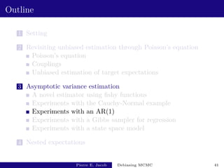
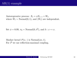
96. AR(1) example
R estimate total cost fishy cost variance of estimator inefficiency
1 [8178 - 10364] [5234 - 5261] [145 - 168] [2.4e+08 - 4.8e+08] [1.3e+12 - 2.5e+12]
10 [9414 - 10250] [6676 - 6756] [1585 - 1667] [4e+07 - 5.5e+07] [2.6e+11 - 3.7e+11]
50 [9748 - 10206] [13148 - 13350] [8069 - 8256] [1.2e+07 - 1.5e+07] [1.6e+11 - 2e+11]
100 [9840 - 10240] [21259 - 21558] [16163 - 16475] [9.2e+06 - 1.1e+07] [2e+11 - 2.4e+11]
Here v(P, h) = 104.
Based on 103 independent replicates, with y = 0.
Pierre E. Jacob Debiasing MCMC 44

97. Comparison to batch means estimators
−2000
−1000
0
1000
2000
1e+04 1e+05 1e+06 1e+07
total cost
bias
BM: # chains 1 2 4 8
BM: r 1 2 3
Pierre E. Jacob Debiasing MCMC 45

98. Comparison to batch means estimators
1e+05
1e+06
1e+07
1e+04 1e+05 1e+06 1e+07
total cost
MSE
BM: # chains 1 2 4 8
BM: r 1 2 3
proposed method (R=50)
Pierre E. Jacob Debiasing MCMC 46

99. Comparison to spectral variance estimators
−2000
−1000
0
1000
2000
1e+04 1e+05 1e+06 1e+07
total cost
bias
SV: # chains 1 2 4 8
SV: r 1 2 3
Pierre E. Jacob Debiasing MCMC 47

100. Comparison to spectral variance estimators
1e+05
1e+06
1e+07
1e+04 1e+05 1e+06 1e+07
total cost
MSE
SV: # chains 1 2 4 8
SV: r 1 2 3
proposed method (R=50)
Pierre E. Jacob Debiasing MCMC 48

101. Outline
1 Setting
2 Revisiting unbiased estimation through Poisson’s equation
Poisson’s equation
Couplings
Unbiased estimation of target expectations
3 Asymptotic variance estimation
A novel estimator using fishy functions
Experiments with the Cauchy-Normal example
Experiments with an AR(1)
Experiments with a Gibbs sampler for regression
Experiments with a state space model
4 Nested expectations
Pierre E. Jacob Debiasing MCMC 48

102. Large-scale Bayesian regression
Biswas, Bhattacharya, Jacob Johndrow, Coupling-based
convergence assessment of some Gibbs samplers for high-dimensional
Bayesian regression with shrinkage priors, 2022.
Linear regression setting, n rows, p columns with p n.
Y ∼ Normal(Xβ, σ2
In),
σ2
∼ InverseGamma(a0/2, b0/2),
ξ−1/2
∼ Cauchy(0, 1)+
,
for j = 1, . . . , p βj ∼ Normal(0, σ2
/ξηj), η
−1/2
j ∼ t(ν)+
.
Global precision ξ, local precision ηj for j = 1, . . . , p.
Pierre E. Jacob Debiasing MCMC 49

103. Large-scale Bayesian regression
Gibbs sampler:
ηj given β, ξ, σ2, for j = 1, . . . , p,
can be sampled exactly or by slice sampling.
Given η1, . . . , ηp,
sample ξ using MRTH step,
sample σ2 given ξ from Inverse-Gamma,
sample β given ξ, σ2 from p-dimensional Normal.
Pierre E. Jacob Debiasing MCMC 50

104. Large-scale Bayesian regression
Gibbs sampler:
ηj given β, ξ, σ2, for j = 1, . . . , p,
can be sampled exactly or by slice sampling.
Given η1, . . . , ηp,
sample ξ using MRTH step,
sample σ2 given ξ from Inverse-Gamma,
sample β given ξ, σ2 from p-dimensional Normal.
Coupling strategy involves common random numbers, maximal
couplings, and “switch to CRN” strategy for η1, . . . , ηp.
Pierre E. Jacob Debiasing MCMC 50

105. Large-scale Bayesian regression
Gibbs sampler:
ηj given β, ξ, σ2, for j = 1, . . . , p,
can be sampled exactly or by slice sampling.
Given η1, . . . , ηp,
sample ξ using MRTH step,
sample σ2 given ξ from Inverse-Gamma,
sample β given ξ, σ2 from p-dimensional Normal.
Coupling strategy involves common random numbers, maximal
couplings, and “switch to CRN” strategy for η1, . . . , ηp.
Riboflavin data: n = 71 responses on p = 4088 predictors.
Bühlmann, Kalish Meier, High-dimensional statistics with a view
toward applications in biology, 2014.
Pierre E. Jacob Debiasing MCMC 50

106. Large-scale Bayesian regression: traceplot
−2.5
−2.0
−1.5
−1.0
−0.5
0.0
0 250 500 750 1000
iteration
β
2564
Pierre E. Jacob Debiasing MCMC 51

107. Large-scale Bayesian regression: TV upper bounds
0.001
0.010
0.100
1.000
0 500 1000 1500 2000
iteration
TV
distance
Pierre E. Jacob Debiasing MCMC 52

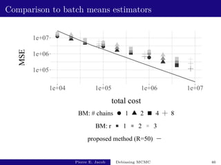
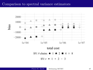
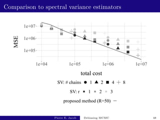
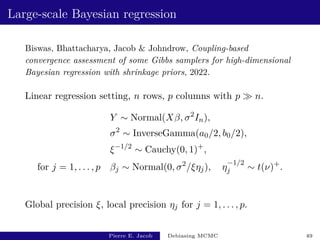
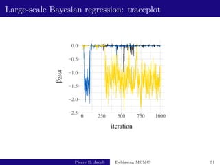
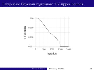
108. Large-scale Bayesian regression: performance
R estimate total cost fishy cost variance of estimator inefficiency
1 [77 - 97] [12308 - 12384] [1521 - 1594] [2.2e+04 - 3.3e+04] [2.7e+08 - 4.1e+08]
5 [78 - 87] [18470 - 18634] [7684 - 7844] [5.4e+03 - 6.8e+03] [9.9e+07 - 1.3e+08]
10 [78 - 85] [26209 - 26444] [15442 - 15656] [2.6e+03 - 3.1e+03] [6.7e+07 - 8.2e+07]
Test function: h : x 7→ β2564.
Based on 103 independent replicates, y ∼ prior.
With k = 500, L = 500, ` = 2500, unbiased MCMC estimators
of π(h) have a mean cost of 5400, and a variance of 0.020,
leading to an inefficiency of 108: not much more than v(P, h).
Pierre E. Jacob Debiasing MCMC 53

109. Outline
1 Setting
2 Revisiting unbiased estimation through Poisson’s equation
Poisson’s equation
Couplings
Unbiased estimation of target expectations
3 Asymptotic variance estimation
A novel estimator using fishy functions
Experiments with the Cauchy-Normal example
Experiments with an AR(1)
Experiments with a Gibbs sampler for regression
Experiments with a state space model
4 Nested expectations
Pierre E. Jacob Debiasing MCMC 53

110. State space model
0
2
4
6
8
0 25 50 75 100
time
response
yt|xt ∼ Binomial(50, (1 + exp(−xt))−1
),
x0 ∼ Normal(0, 1), and ∀t ≥ 1 xt|xt−1 ∼ Normal(αxt−1, σ2
).
Prior is Uniform(0, 1) on α, and σ2 = 1.5 for simplicity.
Test function: h : x 7→ x.
Pierre E. Jacob Debiasing MCMC 54

111. State space model
0
2
4
6
8
0 25 50 75 100
time
response
yt|xt ∼ Binomial(50, (1 + exp(−xt))−1
),
x0 ∼ Normal(0, 1), and ∀t ≥ 1 xt|xt−1 ∼ Normal(αxt−1, σ2
).
Prior is Uniform(0, 1) on α, and σ2 = 1.5 for simplicity.
Test function: h : x 7→ x.
Middleton, Deligiannidis, Doucet, Jacob, Unbiased MCMC for
intractable target distributions, 2020.
Pierre E. Jacob Debiasing MCMC 54

112. State space model: posterior
0
1000
2000
3000
0.92 0.96 1.00
α
count
We try y = 0.5 and y = 0.975 in the definition of
gy(x) = g?(x) − g?(y).
Pierre E. Jacob Debiasing MCMC 55

113. State space model: fishy function
With y = 0.5:
3.75
4.00
4.25
0.900 0.925 0.950 0.975 1.000
α
fishy
function(x)
Pierre E. Jacob Debiasing MCMC 56

114. State space model: fishy function
With y = 0.975:
−0.4
−0.2
0.0
0.900 0.925 0.950 0.975 1.000
α
fishy
function(x)
Pierre E. Jacob Debiasing MCMC 57

115. State space model: asymptotic variance estimator
With y = 0.5:
0
20
40
−0.06 −0.03 0.00 0.03 0.06
estimator of v(P,h)
count
Pierre E. Jacob Debiasing MCMC 58

116. State space model: asymptotic variance estimator
With y = 0.975:
0
20
40
0.001 0.002 0.003 0.004 0.005 0.006
estimator of v(P,h)
count
Pierre E. Jacob Debiasing MCMC 59

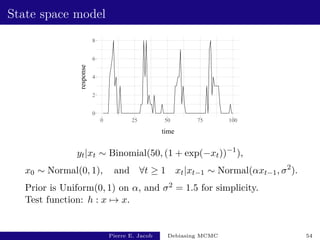
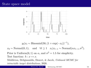
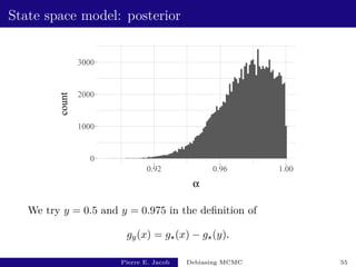
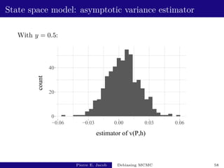
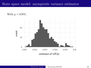
117. State space model: performance
y estimate fishy cost variance of estimator inefficiency
0.5 [2.64e-03 - 5.32e-03] [3.62e+03 - 3.67e+03] [2.2e-04 - 2.8e-04] [1.9e+00 - 2.5e+00]
0.975 [2.85e-03 - 2.99e-03] [1.01e+03 - 1.05e+03] [5.4e-07 - 7.4e-07] [3.3e-03 - 4.5e-03]
Based on 500 independent replicates.
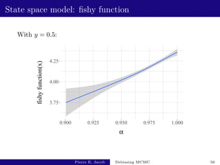
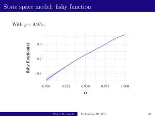
The choice of y has an impact on the performance.
Unbiased MCMC has an inefficiency of 3.8 × 10−3:
not much more than v(P, h).
Pierre E. Jacob Debiasing MCMC 60

118. Outline
1 Setting
2 Revisiting unbiased estimation through Poisson’s equation
Poisson’s equation
Couplings
Unbiased estimation of target expectations
3 Asymptotic variance estimation
A novel estimator using fishy functions
Experiments with the Cauchy-Normal example
Experiments with an AR(1)
Experiments with a Gibbs sampler for regression
Experiments with a state space model
4 Nested expectations
Pierre E. Jacob Debiasing MCMC 60

119. Nested targets
Consider a target distribution that factorizes as
π(x1, x2) = π1(x1)π2(x2|x1).
Pierre E. Jacob Debiasing MCMC 61

120. Nested targets
Consider a target distribution that factorizes as
π(x1, x2) = π1(x1)π2(x2|x1).
Ideal sampling approach:
Sample X1 ∼ π1 perfectly.
Sample X2 ∼ π2(·|X1) perfectly.
Return (X1, X2).
Pierre E. Jacob Debiasing MCMC 61

121. Nested targets
target π(x1, x2) = π1(x1)π2(x2|x1)
Suppose that we can evaluate π1, π2(·|x1) up to normalization.
Pierre E. Jacob Debiasing MCMC 62

122. Nested targets
target π(x1, x2) = π1(x1)π2(x2|x1)
Suppose that we can evaluate π1, π2(·|x1) up to normalization.
MCMC approach:
Sample X1 ∼ π1 using MCMC.
Sample X2 ∼ π2(·|X1) using MCMC.
Return (X1, X2).
Pierre E. Jacob Debiasing MCMC 62

123. Nested targets
target π(x1, x2) = π1(x1)π2(x2|x1)
Suppose that we can evaluate π1, π2(·|x1) up to normalization.
MCMC approach:
Sample X1 ∼ π1 using MCMC.
Sample X2 ∼ π2(·|X1) using MCMC.
Return (X1, X2).
Consistent as numbers of iterations at both stages go to infinity.
Awkward tuning, convergence diagnostics, error estimation.
Pierre E. Jacob Debiasing MCMC 62

124. Nested targets
target π(x1, x2) = π1(x1)π2(x2|x1)
If π1 = πu
1 /Z1 and π2(·|x1) = πu
2 (·|x1)/Z2(x1), and we can
evaluate πu
1 , πu
2 (·|x1), but not Z2(x1), then
π(x1, x2) =
πu
1 (x1)
Z1
πu
2 (x2|x1)
Z2(x1)
is intractable. Not easy to generate a π-invariant chain.
Pierre E. Jacob Debiasing MCMC 63

125. Nested targets
target π(x1, x2) = π1(x1)π2(x2|x1)
If π1 = πu
1 /Z1 and π2(·|x1) = πu
2 (·|x1)/Z2(x1), and we can
evaluate πu
1 , πu
2 (·|x1), but not Z2(x1), then
π(x1, x2) =
πu
1 (x1)
Z1
πu
2 (x2|x1)
Z2(x1)
is intractable. Not easy to generate a π-invariant chain.
Plummer, Cuts in Bayesian graphical models, 2014.
Liu Goudie, Stochastic approximation cut algorithm for inference in
modularized Bayesian models, 2021.
Pierre E. Jacob Debiasing MCMC 63

126. Nested expectation: cut distribution
First module:
parameter θ1, data Y1
prior: p1(θ1)
likelihood: p1(Y1|θ1)
Second module:
parameter θ2, data Y2
prior: p2(θ2|θ1)
likelihood: p2 (Y2|θ1, θ2)
Pierre E. Jacob Debiasing MCMC 64

127. Nested expectation: cut distribution
One might want to propagate uncertainty without allowing
“feedback” of second module on first module.
In epidemiology, PKPD, multiple imputation of missing data,
generated regressors, causal inference with propensity scores,
multiphase inteference. . .
Cut distribution:
πcut
(θ1, θ2; Y1, Y2) = p1(θ1|Y1)p2 (θ2|θ1, Y2).
Different from the posterior distribution under joint model,
under which the first marginal is π(θ1|Y1, Y2).
Plummer, Cuts in Bayesian graphical models, 2014.
Pierre E. Jacob Debiasing MCMC 65

128. Nested targets
target π(x1, x2) = π1(x1)π2(x2|x1)
Pierre E. Jacob Debiasing MCMC 66

129. Nested targets
target π(x1, x2) = π1(x1)π2(x2|x1)
Obtain π̂1 =
PN1
k=1 ω1,kδX1,k
approximating π1.
Draw K uniformly in {1, . . . , N1}.
Obtain π̂2 =
PN2
n=1 ω2,nδX2,n approximating π2(·|X1,K).
Pierre E. Jacob Debiasing MCMC 66

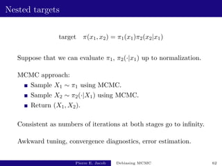
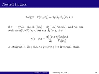
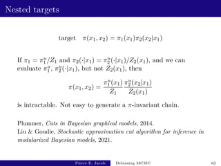
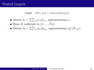
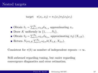
130. Nested targets
target π(x1, x2) = π1(x1)π2(x2|x1)
Obtain π̂1 =
PN1
k=1 ω1,kδX1,k
approximating π1.
Draw K uniformly in {1, . . . , N1}.
Obtain π̂2 =
PN2
n=1 ω2,nδX2,n approximating π2(·|X1,K).
Then E[N1ω1,K
N2
X
n=1
ω2,nh(X1,K, X2,n)]
= E[E[N1ω1,K
N2
X
n=1
ω2,nh(X1,K, X2,n)|π̂1]]
= E[
N1
X
k=1
ω1,k
Z
h(X1,k, x2)π2(dx2|X1,k)] = π(h).
Pierre E. Jacob Debiasing MCMC 66

131. Nested targets
target π(x1, x2) = π1(x1)π2(x2|x1)
Obtain π̂1 =
PN1
k=1 ω1,kδX1,k
approximating π1.
Draw K uniformly in {1, . . . , N1}.
Obtain π̂2 =
PN2
n=1 ω2,nδX2,n approximating π2(·|X1,K).
Return N1ω1,K
PN2
n=1 ω2,nh(X1,K, X2,n).
Pierre E. Jacob Debiasing MCMC 67

132. Nested targets
target π(x1, x2) = π1(x1)π2(x2|x1)
Obtain π̂1 =
PN1
k=1 ω1,kδX1,k
approximating π1.
Draw K uniformly in {1, . . . , N1}.
Obtain π̂2 =
PN2
n=1 ω2,nδX2,n approximating π2(·|X1,K).
Return N1ω1,K
PN2
n=1 ω2,nh(X1,K, X2,n).
Consistent for π(h) as number of independent repeats → ∞.
Still awkward regarding tuning, but easier regarding
convergence diagnostics and error estimation.
Pierre E. Jacob Debiasing MCMC 67

133. Discussion
Douc, Jacob, Lee Vats,
Solving the Poisson equation using coupled Markov chains, on arXiv.
Estimate friendly fishes with faithful couplings.
Novel asymptotic variance estimator does not require long
runs, and shows promising performance.
Unbiased estimators are convenient for nested expectations.
Pierre E. Jacob Debiasing MCMC 68

134. Discussion
Douc, Jacob, Lee Vats,
Solving the Poisson equation using coupled Markov chains, on arXiv.
Estimate friendly fishes with faithful couplings.
Novel asymptotic variance estimator does not require long
runs, and shows promising performance.
Unbiased estimators are convenient for nested expectations.
Opportunities at ESSEC:
Open-rank faculty position in stats/econometrics.
PhD program in data analytics.
Thank you for listening!
Pierre E. Jacob Debiasing MCMC 68