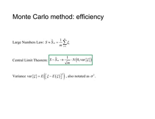
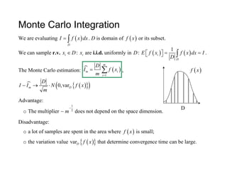
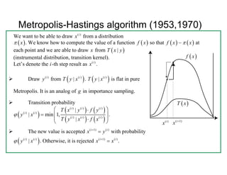
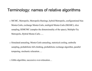
Markov Chain Monte Carlo (MCMC) methods use Markov chains to sample from probability distributions for use in Monte Carlo simulations. The Metropolis-Hastings algorithm proposes transitions to new states in the chain and either accepts or rejects those states based on a probability calculation, allowing it to sample from complex, high-dimensional distributions. The Gibbs sampler is a special case of MCMC where each variable is updated conditional on the current values of the other variables, ensuring all proposed moves are accepted. These MCMC methods allow approximating integrals that are difficult to compute directly.

1. Markov Chain Monte-Carlo
(MCMC)
What for is it and what does it look like?
A. Favorov, 2003-2014 favorov@sensi.org
favorov@gmail.com

2. Monte Carlo method: a figure square
The value  is unknown.
Let’s sample a random value (r.v.)  :
   
 
 
, : i.i.d. as flat 0,1
1 ,
0 ,
 
 
  

  
x y
x y
x y
Clever notation:  ,  I x y
i.i.d. is “Identically Independently Distributed”
Expectation of  :        E S S
1
μ
1

3. Monte Carlo method: efficiency
Large Numbers Law: 
1
1


  
m
m i
i
S S
m
Central Limit Theorem:    
1
0,var   mS S N
m
Variance     2
var      E E , also notated as 2
 .

4. Monte Carlo Integration
We are evaluating   D
I f x dx. D is domain of  f x or its subset.
We can sample r.v. ix D: ix are i.i.d. uniformly in D:    
1
    i
D
E f x f x dx I
D
.
The Monte Carlo estimation:   
1
 
m
m i
i
D
I f x
m
,
    0,var  m D
D
I I N f x
m
Advantage:
o The multiplier
1
2

 m does not depend on the space dimension.
Disadvantage:
o a lot of samples are spent in the area where  f x is small;
o the variation value   varD f x that determine convergence time can be large.
D
 f x

5. Monte Carlo importance integration
We are evaluating   D
I f x dx
Let’s sample ix D from a “trial” distribution  g x that “looks like”  f x and
   0 0  f x g x . ix i.i.d. in D as  g x that “resembles”  f x
Thus
 
 
 
 
   
 
  
 
 
i
g
i D D
f x f x
E g x dx f x dx
g x g x
.
MC evaluation:   
 1
1

 
m
i
m
i i
f x
I
m g x
;   
 
1
0,varm D
f x
I I N
g xm
  
      
  
“More uniform” means “better”.

6. Another example of importance integration
We are evaluating       
   E h x h x x dx, where   x is a distribution,
e.g.   1x dx 
sample ix from a distribution  .g so that    0 0   x g x
Importance weight    i i iw x g x ;   
 
 
  1g
x
E w x g x dx
g x

 
   
 
           
1 1 1 1
1 1m m m m
i
m i i i i i i
i i i ii
x
h x w x h x w x h x w x
m g x m


   
     
           
1 1 1
1 m m m
m i i i i i
i i i
w x h x w x h x w x
m

  
   
Sampling from   x :   
1
1 m
m i
i
h x
m


 

7. Rejection sampling (Von Neumann, 1951)
We have a distribution   x and
we want to sample from it.
We are able to calculate   ( ) f x c x for x. Any c.
We are able to sample      , : g x M Mg x f x .
Thus, we can sample   x :
Draw a value x from  g x .
Accept the value x with the probability    f x Mg x .
     
 
 
 |

      
c x c
P accept P accept x P x dx g x dx
Mg x M
 
   
 
 
 
   
|
|


 
    
P accept x P x c x M
P x accept g x x
P accept Mg x c
 g x
  x
 f x

8. Metropolis-Hastings algorithm (1953,1970)
We want to be able to draw ( )i
x from a distribution
 x . We know how to compute the value of a function  f x so that    f x x at
each point and we are able to draw x from  |T x y
(instrumental distribution, transition kernel).
Let’s denote the i-th step result as ( )i
x .
 Draw ( )i
y from  ( )
| i
T y x .  ( )
| i
T y x is flat in pure
Metropolis. It is an analog of g in importance sampling.
 Transition probability
 
   
   
( ) ( ) ( )
( ) ( )
( ) ( ) ( )
|
| min 1,
|

 
  
  
i i i
i i
i i i
T x y f y
y x
T y x f x
.
 The new value is accepted ( 1) ( )
i i
x y with probability
 ( ) ( )
| i i
y x . Otherwise, it is rejected ( 1) ( )
i i
x x .
( 1)i
x ( )i
x
 f x
 T x

9. Why does it work: the local balance
Let’s show that if x is already distributed as     x f x , then the MH algorithm
keeps the distribution.
Local balance condition for two points x and y :
           | | | |     f x T y x y x f y T x y x y . Let’s check it:
         
   
   
              
|
| | | min 1,
|
min | , | | |
T x y f y
f x T y x y x f x T y x
T y x f x
T y x f x T x y f y f y T x y x y


 
      
 
     
The balance is stable:
     | | f x T y x y x is the flow from x to y and
     | | f y T x y x y is the flow from y to x.
The stable local balance is enough (BTW, it is not a necessary condition).

10. Markov chains, Maximization, Simulated
Annealing
ix created as described above is a Markov chain (MC) with transition kernel
   ( 1) ( ) ( 1) ( )
| |  
i i i i
x x T x x . The fact that the chain has a stationary distribution and the
convergence of the chain to the distribution can be proved by the MC theory methods.
Minimization.  C x is a cost (a fine).  
  min
exp
 
  
 
C x C
f x
t
.
We can characterize the transition kernel with a temperature. Then we can decrease the
temperature step-by-step (simulated annealing). MCMC and SA are very effective for
optimization since gradient methods use to be locked is a local maximum while pure
MC is extremely ineffective.

11. MCMC prior and Bayesian paradigm
( | ) ( )
( | ) ( | ) ( )
( )
posterior likelihood prior
P D M P M
P M D P D M P M
P D

  
 
here, evidence
MCMC and its variations are often used for the best model search .
Let’s can formulate some requirements for the algorithm and thus for the transition
kernel:
o We want it not to depend on the current data.
o We want to minimize the rejection rate.
So, an effective transition kernel is so that the prior ( )P M is its stationary distribution.

12. Terminology: names of relative algorithms
o MCMC, Metropolis, Metropolis-Hastings, hybrid Metropolis, configurational bias
Monte-Carlo, exchange Monte-Carlo, multigrid Monte-Carlo (MGMC), slice
sampling, RJMCMC (samples the dimensionality of the space), Multiple-Try
Metropolis, Hybrid Monte-Carlo…..
o Simulated annealing, Monte-Carlo annealing, statistical cooling, umbrella
sampling, probabilistic hill climbing, probabilistic exchange algorithm, parallel
tempering, stochastic relaxation….
o Gibbs algorithm, successive over-relaxation…

13. Gibbs Sampler (Geman and Geman, 1984)
Now, x is a k -dimensional variable  1 2, .... kx x x .
Let’s denote  1 2 1 1, .., , ,.. ,1    m m m kx x x x x x m k
On each step of the Markov Chain we choose the “current coordinate” im .
Then, we calculate the distribution  ( )
| i i
i
m mf x x and draw the next value ( )
i
i
my from the
distribution.
All other coords are the same as on the previous step, ( ) ( )
 i i
i i
m my x .
For such a transition kernel,
 
   
   
( ) ( ) ( )
( ) ( )
( ) ( ) ( )
|
| min 1, 1
|

 
  
  
i i i
i i
i i i
T x y f y
y x
T y x f x
.
o We have no rejects, so the procedure is very effective.
o The “temperature” decreases rather fast .

14. Inverse transform sampling (well-known)
We want to sample from the density  x . We know how to calculate the inverse
function for the cumulative distribution.
Generate a random number from the  0,1 uniform distribution; call this iu .
Compute the value ix such that  
ix
ix dx u


 ix is the random number that is drawn from the distribution described by   x .
 x dx
u
1
0
ix x
   
   
   
, ,x x x u u u
p x x uniform u u
u
p x uniform x
x

    
  

  


15. Slice sampling (Neal, 2003)
Sampling of x from  f x is equivalent to sampling of  ,x y pairs from they area.
So, we introduce an auxiliary variable y and iterate as follows:
for a sample tx we choose ty uniformly from the interval  0, tf x  
given ty we choose 1ix uniformly at random from   : tx f x y
the sample of x distributed as  f x is obtained by ignoring the y values.

16. Literature
Liu, J.S. (2002) Monte Carlo Strategies in Scientific Computing. Springer-Verlag, NY, Berlin, Heidelberg.
Robert, C.P. (1998) Discretization and MCMC Convergence Assessment, Springer-Verlag.
Laarhoven, van, P.M.J. and Aarts, E.H.L (1988) Simulated Annealing: Theory and Applications. Kluwer Academic
Publishers.
Geman, S and Geman, D (1984). Stochastic relaxation, Gibbs distribution and the Bayesian restoration of images. IEEE
Transactions on Pattern Analysis and Machine Intelligence. 6, 621-641.
Besag, J., Green, P., Higdon, D., and Mengersen, K. (1996) Bayesian computation and Stochastic Sytems. Statistical Science,
10, 1, 3-66.
Lawrence, C.E., Altschul, S.F., Boguski, M.S., Liu, J.S., Neuwald, A.F., and Wootton, J.C. (1993). Detecting subtle sequence
signals: a Gibbs sampling strategy for multiple alignment. Science 262, 208-214.
Sivia, D.S. (1996) Data Analysis. A Bayesian tutorial. Clarendon Press, Oxford.
Neal, Radford M. (2003) Slice Sampling. The Annals of Statistics 31(3):705-767.
http://civs.ucla.edu/MCMC/MCMC_tutorial.htm
Sheldon Ross. A First Course in Probability
Соболь И.М. Метод Монте-Карло
Sometimes, it works 
Favorov, A.V., Andreewski, T.V., Sudomoina, M.A., Favorova O.O., Parmigiani, G. Ochs, M.F. (2005). A Markov chain
Monte Carlo technique for identification of combinations of allelic variants underlying complex diseases in humans. Genetics
171(4): 2113-21.
Favorov, A.V., Gelfand, M.S., Gerasimova, A.V. Ravcheev, D.A., Mironov, A.A., Makeev, V. J. (2005). A Gibbs sampler
for identification of symmetrically structured, spaced DNA motifs with improved estimation of the signal length.
Bioinformatics 21(10): 2240-2245.