Bayesian Techniques for Parameter Estimation
Statistical Inference
Goal: The goal in statistical inference is to make conclusions about a
phenomenon based on observed data.
Frequentist: Observations made in the past are analyzed with a specified
model. Result is regarded as confidence about state of real world.
• Probabilities defined as frequencies with which an event occurs if experiment
is repeated several times.
• Parameter Estimation:
o Relies on estimators derived from different data sets and a specific sampling
distribution.
o Parameters may be unknown but are fixed and deterministic.
Bayesian: Interpretation of probability is subjective and can be updated with
new data.
• Parameter Estimation: Parameters are considered to be random variables
having associated densities.
e
Bayesian Inference: Simple Model
Example: Displacement-force relation (Hooke’s Law)
Parameter: Stiffness E
Strategy: Use model fit to data to update prior information
Prior Information
Information Provided
by Model and Data
Updated Information
Non-normalized Bayes’ Relation:
ModelData
s(MPa)
⇡0(E) e-
PN
i=1[si -Eei ]2
/2 2
⇡(E|s)
⇡(E|s) = e-
PN
i=1[si -Eei ]2
/2 2
⇡0(E)
si = Eei + "i , i = 1, ... , N
"i ⇠ N(0, 2
)
Bayesian Inference
Bayes Relation: Specifies posterior in terms of likelihood and prior
• Prior Distribution: Quantifies prior knowledge of parameter values
• Likelihood: Probability of observing a data given set of parameter values.
• Posterior Distribution: Conditional distribution of parameters given observed data.
Problem: Can require high-dimensional integration
• e.g., MFC Model: p = 20!
• Solution: Sampling-based Markov Chain Monte Carlo (MCMC) algorithms.
• Metropolis algorithms first used by nuclear physicists during Manhattan Project
in 1940’s to understand particle movement underlying first atomic bomb.
Posterior
Distribution
Normalization Constant
Prior Distribution
Likelihood: e-
PN
i=1[si -Eei ]2
/2 2
, q = E
= [s1, ... , sN ]
⇡(q| ) =
⇡( |q)⇡0(q)
R
Rp ⇡( |q)⇡0(q)dq
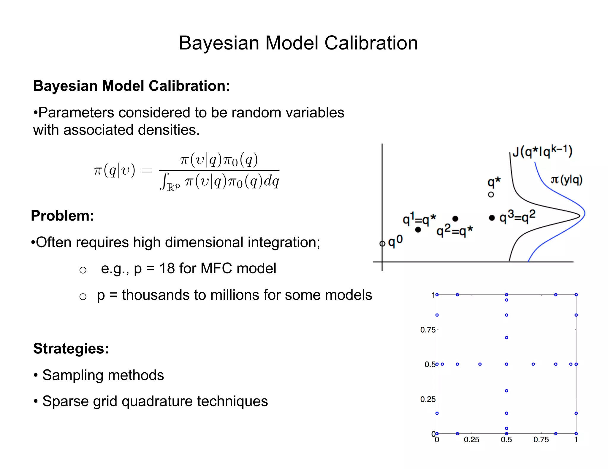
Bayesian Model Calibration
Bayesian Model Calibration:
• Parameters assumed to be random variables
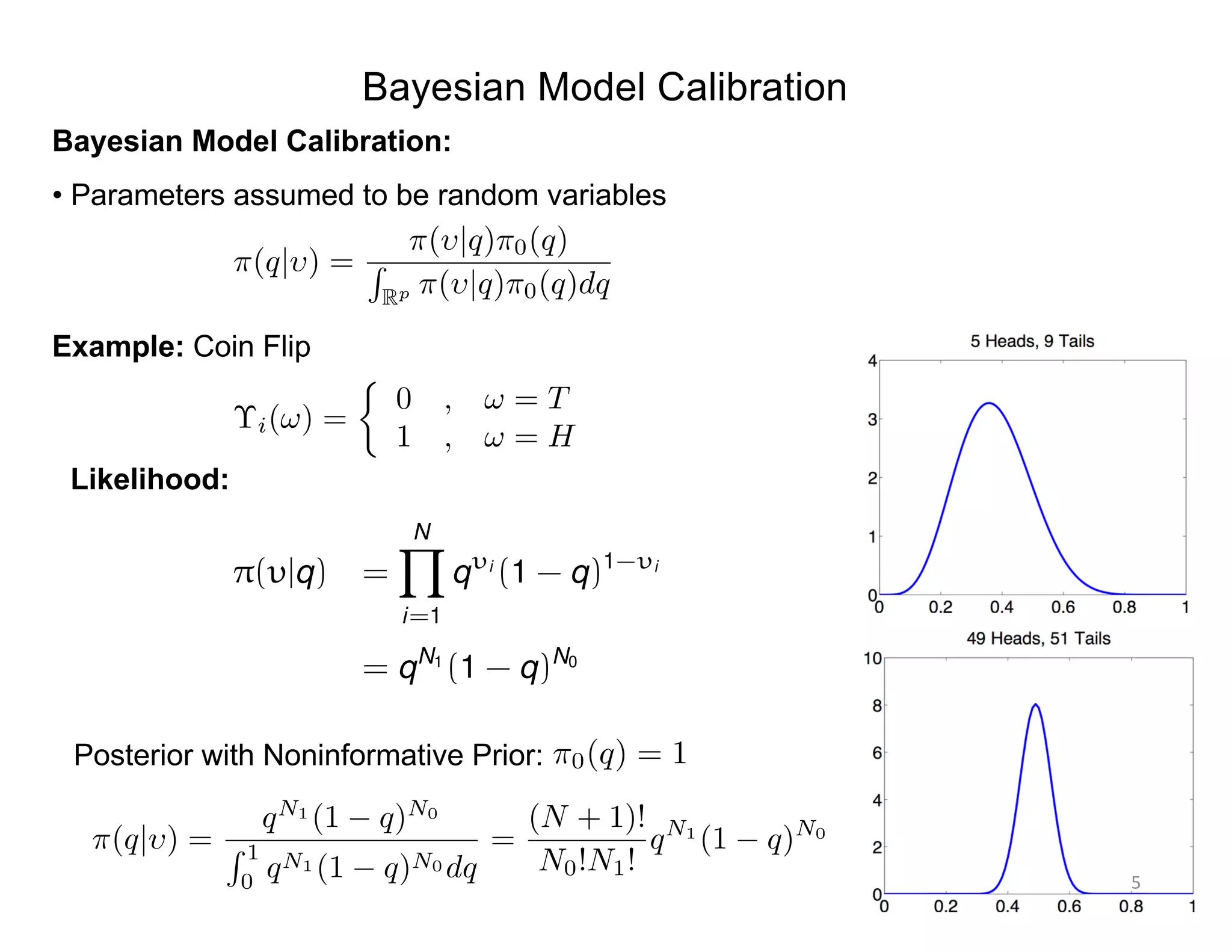
Example: Coin Flip
⇡(q| ) =
⇡( |q)⇡0(q)
R
Rp ⇡( |q)⇡0(q)dq
⌥i(!) =
⇢
0 , ! = T
1 , ! = H
Likelihood:
Posterior with Noninformative Prior:
⇡(q| ) =
qN1
(1 q)N0
R 1
0
qN1 (1 q)N0 dq
=
(N + 1)!
N0!N1!
qN1
(1 q)N0
⇡0(q) = 1
⇡( |q) =
NY
i=1
q i
(1 - q)1- i
= qN1
(1 - q)N0
5
Bayesian Inference
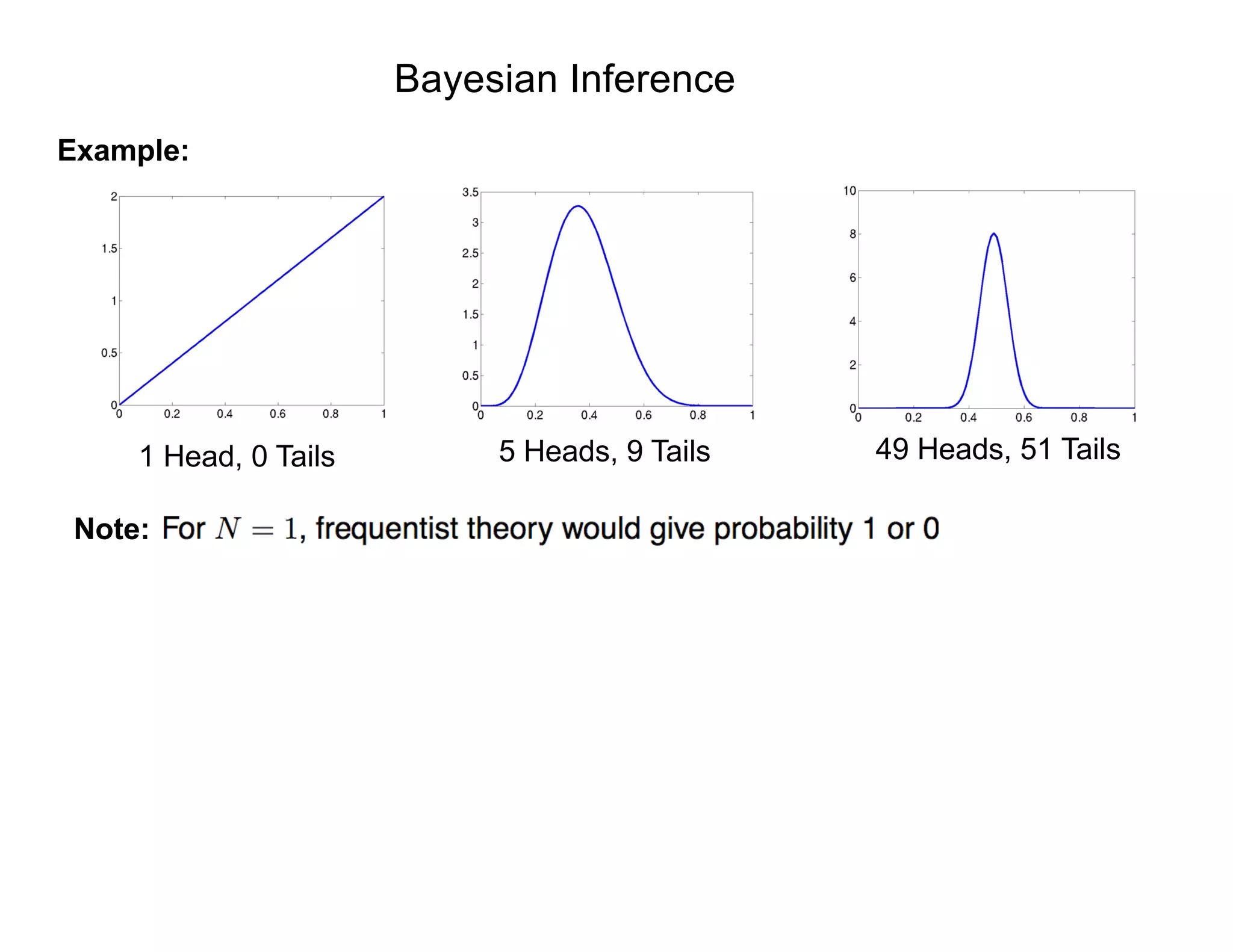
Example:
1 Head, 0 Tails 5 Heads, 9 Tails 49 Heads, 51 Tails
Note:
Bayesian Inference
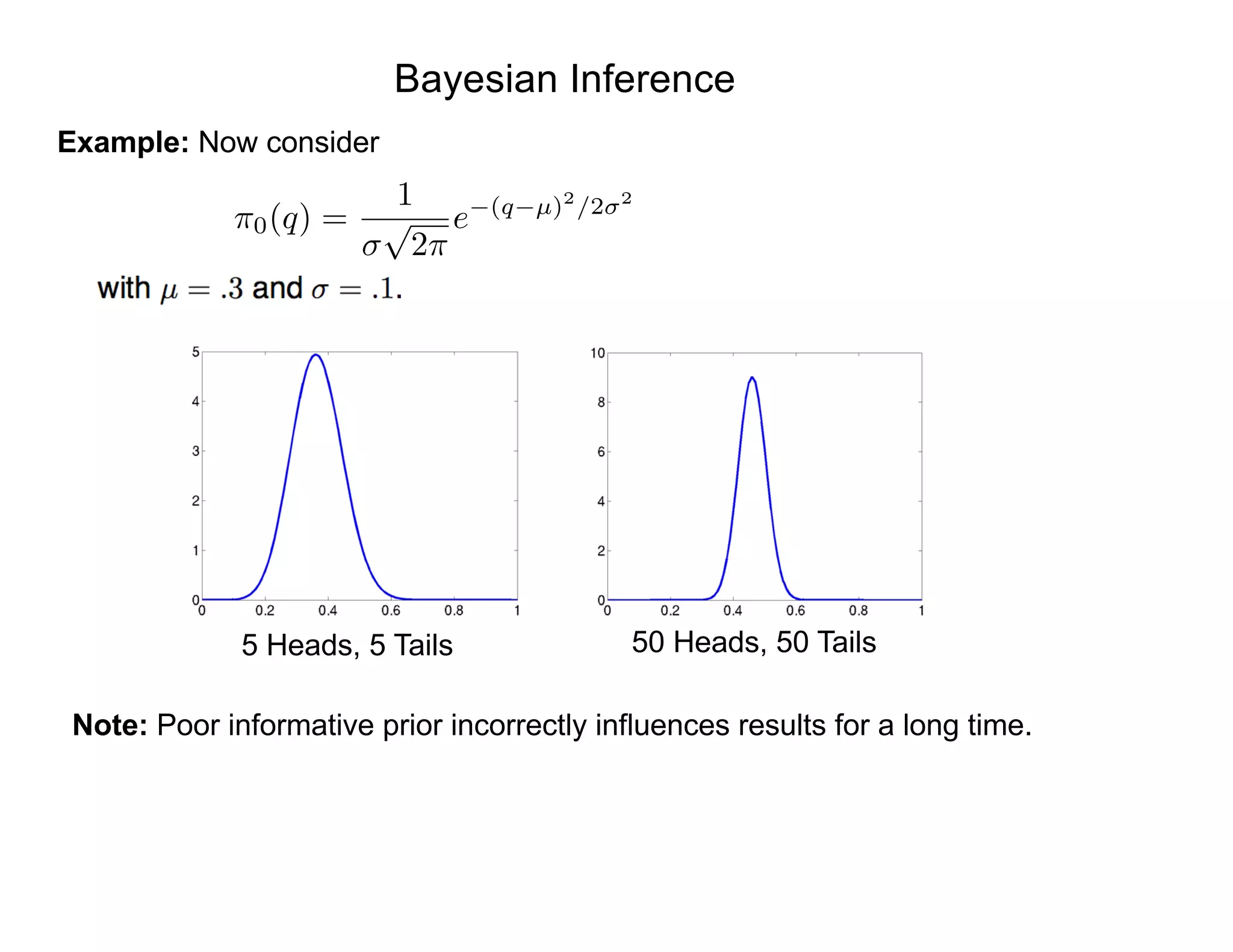
Example: Now consider
Note: Poor informative prior incorrectly influences results for a long time.
50 Heads, 50 Tails5 Heads, 5 Tails
⇡0(q) =
1
p
2⇡
e (q µ)2
/2 2
Likelihood:
Assumption: Assume that measurement errors are iid and
Parameter Estimation Problem
"i ⇠ N(0, 2
)
⇡( |q) = L(q, | ) =
1
(2⇡ 2)n/2
e SSq/2 2
SSq =
nX
i=1
[ i fi(q)]
2
is the sum of squares error.
where
Parameter Estimation: Example
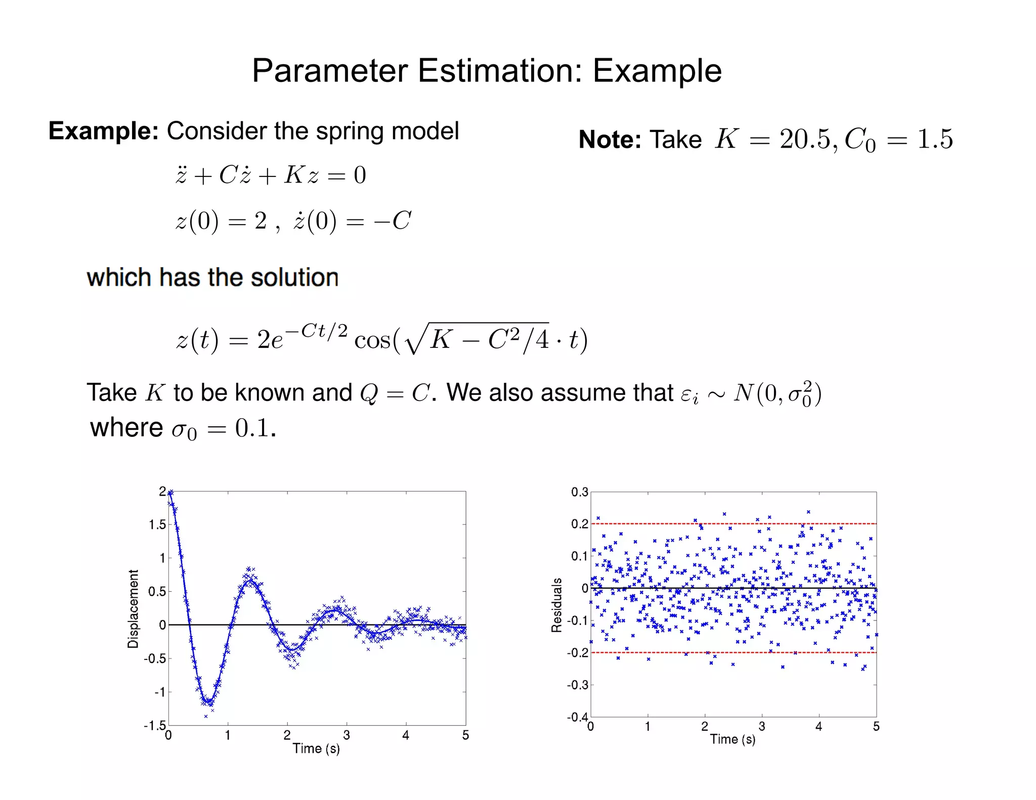
Example: Consider the spring model
¨z + C ˙z + Kz = 0
z(0) = 2 , ˙z(0) = C
z(t) = 2e Ct/2
cos(
p
K C2/4 · t)
Note: Take K = 20.5, C0 = 1.5
Take K to be known and Q = C. We also assume that "i ⇠ N(0, 2
0)
where 0 = 0.1.
Parameter Estimation: Example
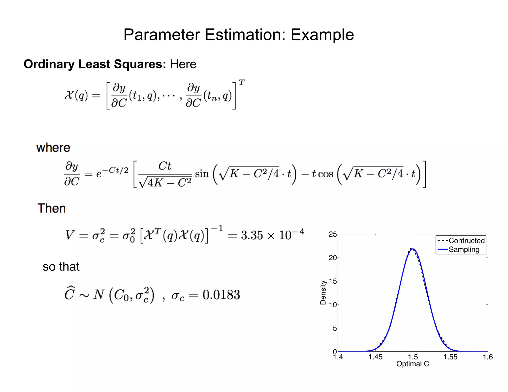
Ordinary Least Squares: Here
1.4 1.45 1.5 1.55 1.6
0
5
10
15
20
25
Optimal C
Density
Contructed
Sampling
so that
Parameter Estimation: Example
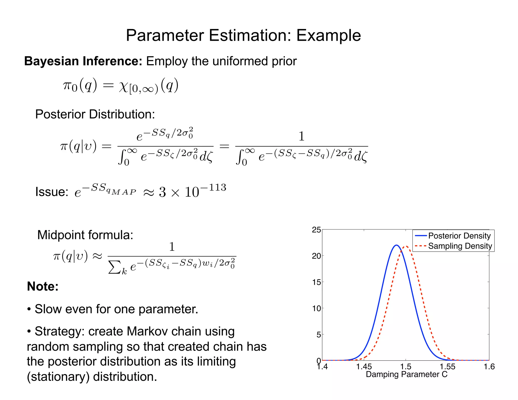
Bayesian Inference: Employ the uniformed prior
Note:
• Slow even for one parameter.
• Strategy: create Markov chain using
random sampling so that created chain has
the posterior distribution as its limiting
(stationary) distribution.
⇡0(q) = [0,1)(q)
Posterior Distribution:
⇡(q| ) =
e SSq/2 2
0
R 1
0
e SS⇣ /2 2
0 d⇣
=
1
R 1
0
e (SS⇣ SSq)/2 2
0 d⇣
Midpoint formula:
⇡(q| ) ⇡
1
P
k e (SS⇣i
SSq)wi/2 2
0
Issue: e SSqMAP ⇡ 3 ⇥ 10 113
1.4 1.45 1.5 1.55 1.6
0
5
10
15
20
25
Damping Parameter C
Posterior Density
Sampling Density
Bayesian Model Calibration
Bayesian Model Calibration:
•Parameters considered to be random variables
with associated densities.
Problem:
•Often requires high dimensional integration;
o e.g., p = 18 for MFC model
o p = thousands to millions for some models
Strategies:
• Sampling methods
• Sparse grid quadrature techniques
⇡(q| ) =
⇡( |q)⇡0(q)
R
Rp ⇡( |q)⇡0(q)dq
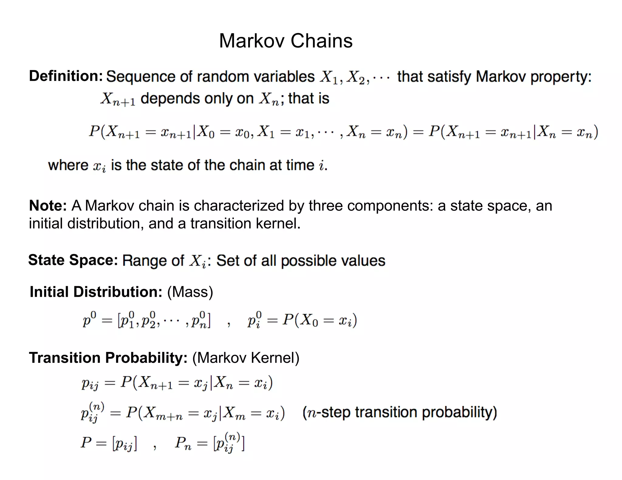
Markov Chains
Definition:
Note: A Markov chain is characterized by three components: a state space, an
initial distribution, and a transition kernel.
State Space:
Initial Distribution: (Mass)
Transition Probability: (Markov Kernel)
Markov Chain Techniques
Markov Chain: Sequence of events where current state depends only on last value.
Baseball:
• Assume that team which won last game has 70% chance of winning next game and
30% chance of losing next game.
• Assume losing team wins 40% and loses 60% of next games.
• Percentage of teams who win/lose next game given by
• Question: does the following limit exist?
States are S = {win,lose}. Initial state is p0
= [0.8, 0.2].
0.7 win lose
0.4
0.3
0.6
p1
= [0.8 , 0.2]

0.7 0.3
0.4 0.6
= [0.64 , 0.36]
pn
= [0.8 , 0.2]

0.7 0.3
0.4 0.6
n
Markov Chain Techniques
Baseball Example: Solve constrained relation
⇡ = ⇡P ,
X
⇡i = 1
) [⇡win , ⇡lose]

0.7 0.3
0.4 0.6
= [⇡win , ⇡lose] , ⇡win + ⇡lose = 1
to obtain
⇡ = [0.5714 , 0.4286]
Markov Chain Techniques
Baseball Example: Solve constrained relation
⇡ = ⇡P ,
X
⇡i = 1
) [⇡win , ⇡lose]

0.7 0.3
0.4 0.6
= [⇡win , ⇡lose] , ⇡win + ⇡lose = 1
to obtain
⇡ = [0.5714 , 0.4286]
Alternative: Iterate to compute solution
n pn
n pn
n pn
0 [0.8000 , 0.2000] 4 [0.5733 , 0.4267] 8 [0.5714 , 0.4286]
1 [0.6400 , 0.3600] 5 [0.5720 , 0.4280] 9 [0.5714 , 0.4286]
2 [0.5920 , 0.4080] 6 [0.5716 , 0.4284] 10 [0.5714 , 0.4286]
3 [0.5776 , 0.4224] 7 [0.5715 , 0.4285]
Notes:
• Forms basis for Markov Chain Monte Carlo (MCMC) techniques
• Goal: construct chains whose stationary distribution is the posterior density
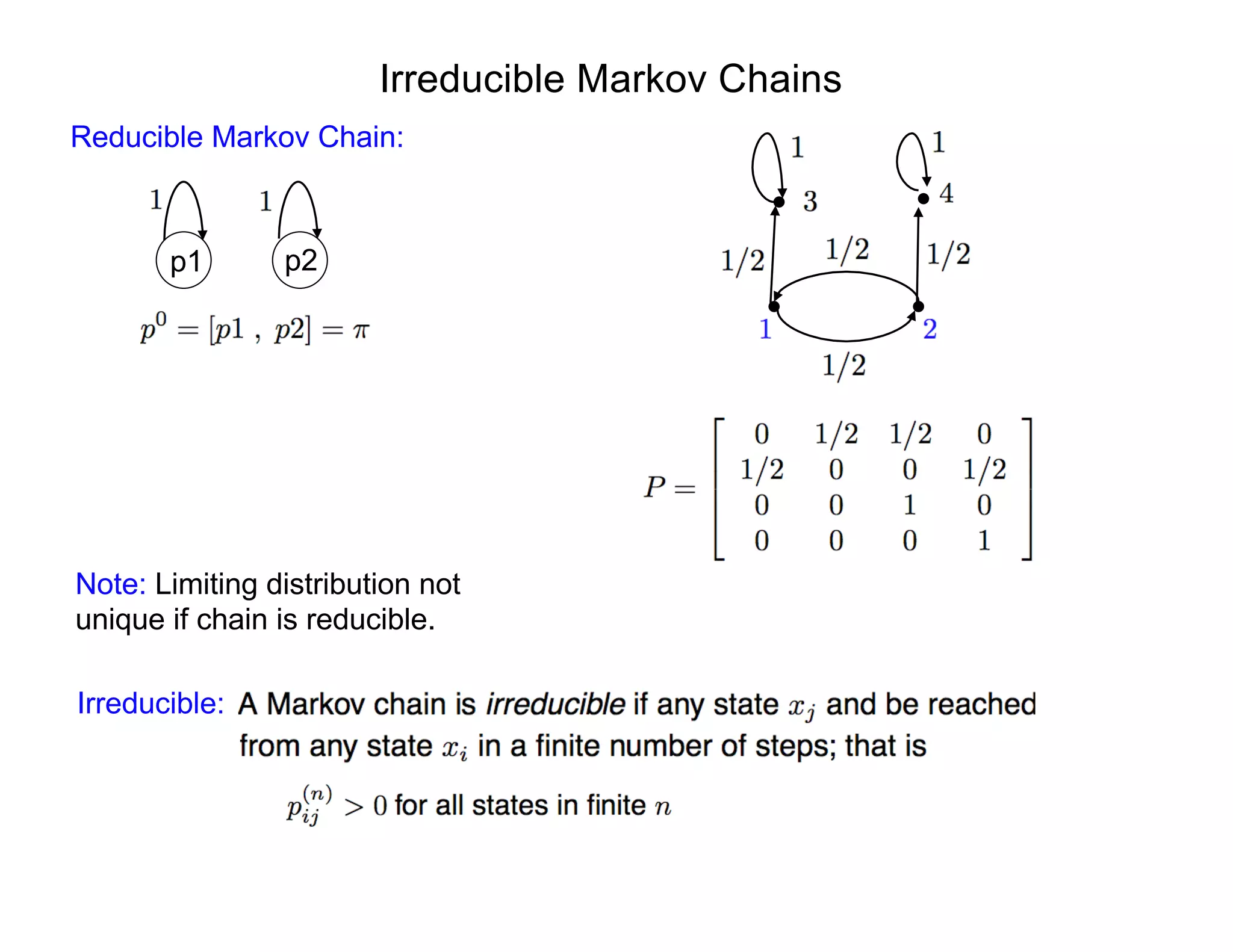
Irreducible Markov Chains
Irreducible:
Reducible Markov Chain:
p1 p2
Note: Limiting distribution not
unique if chain is reducible.
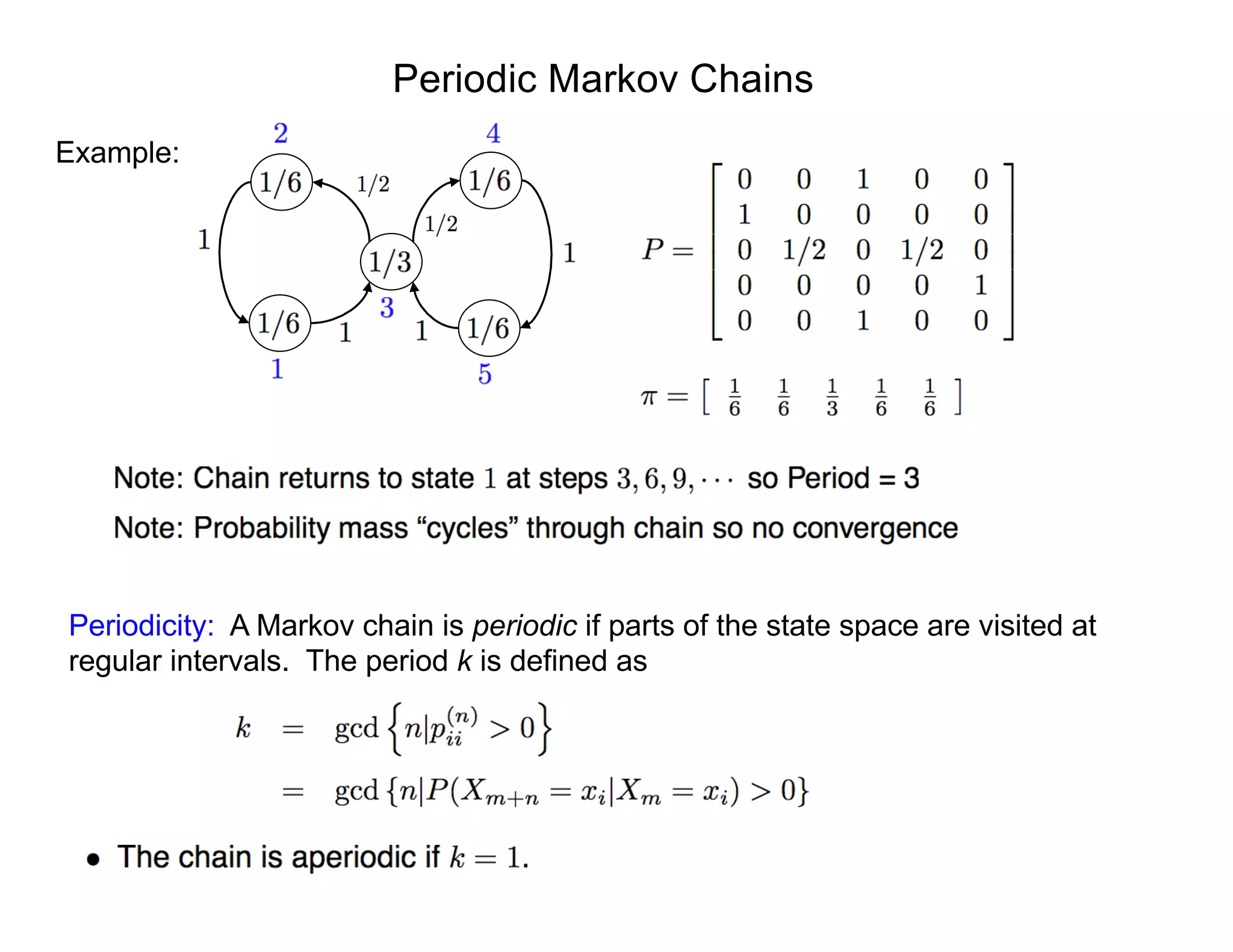
Periodic Markov Chains
Example:
Periodicity: A Markov chain is periodic if parts of the state space are visited at
regular intervals. The period k is defined as
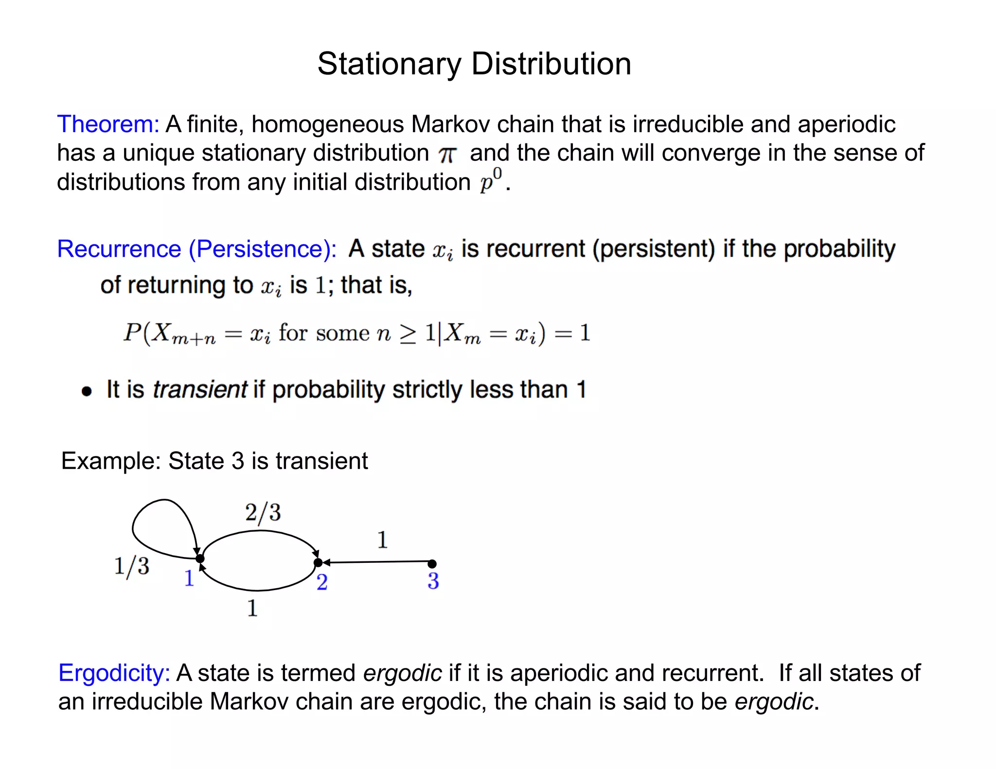
Stationary Distribution
Theorem: A finite, homogeneous Markov chain that is irreducible and aperiodic
has a unique stationary distribution and the chain will converge in the sense of
distributions from any initial distribution .
Recurrence (Persistence):
Example: State 3 is transient
Ergodicity: A state is termed ergodic if it is aperiodic and recurrent. If all states of
an irreducible Markov chain are ergodic, the chain is said to be ergodic.
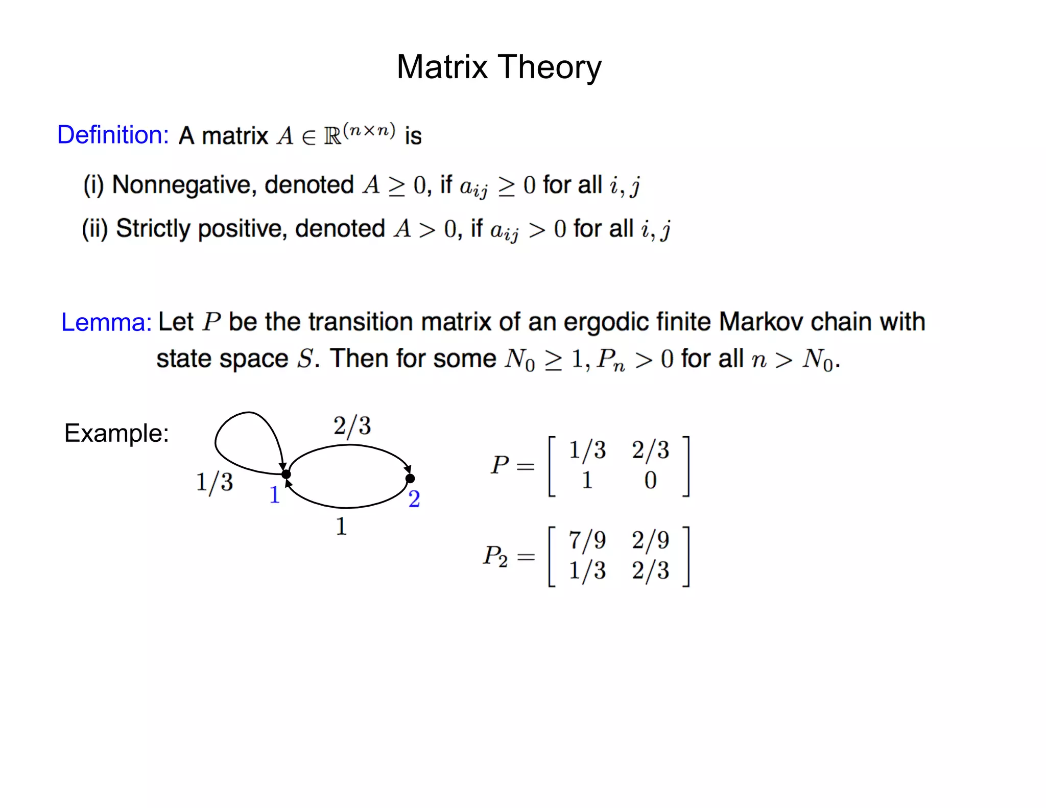
Matrix Theory
Definition:
Lemma:
Example:
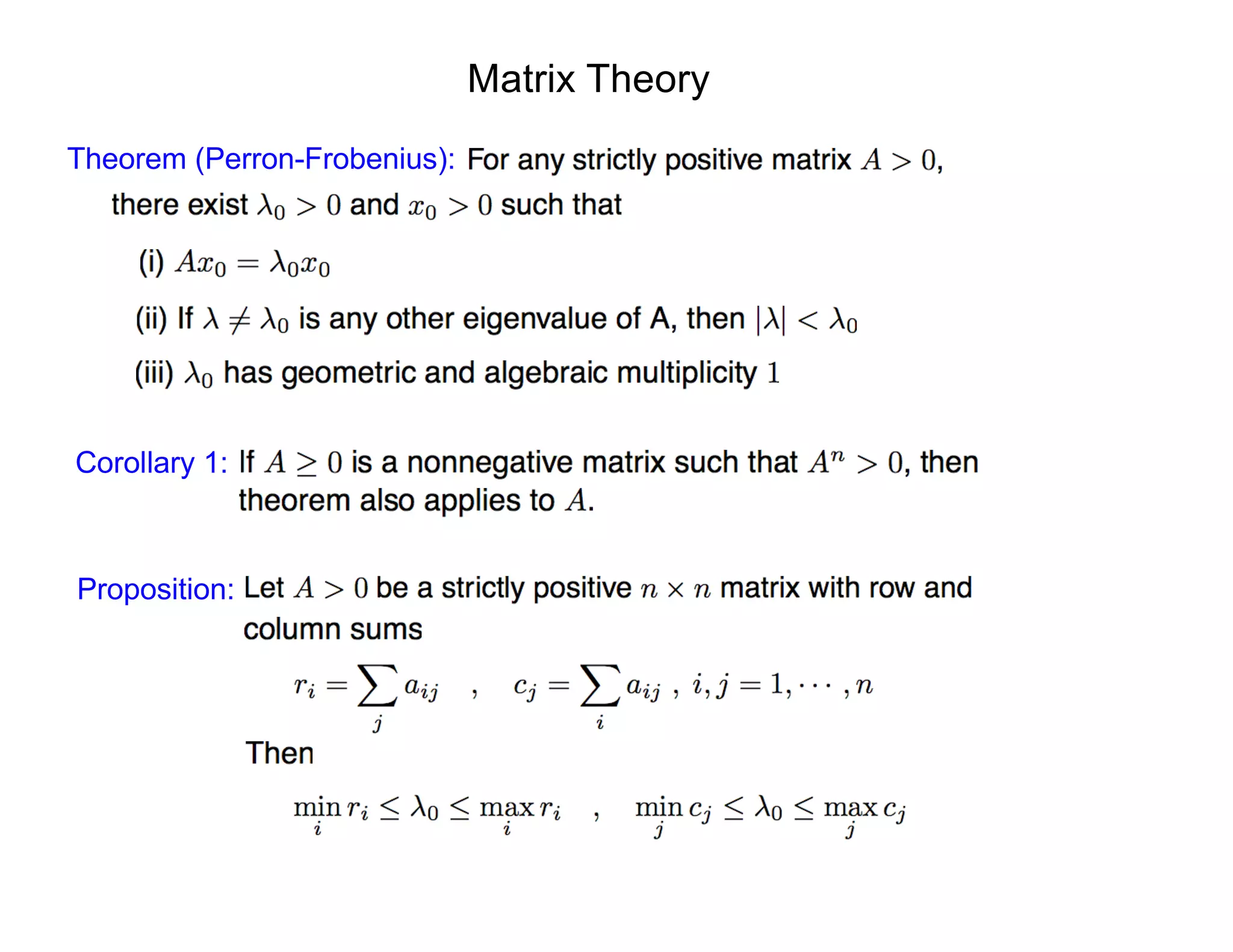
Matrix Theory
Theorem (Perron-Frobenius):
Corollary 1:
Proposition:
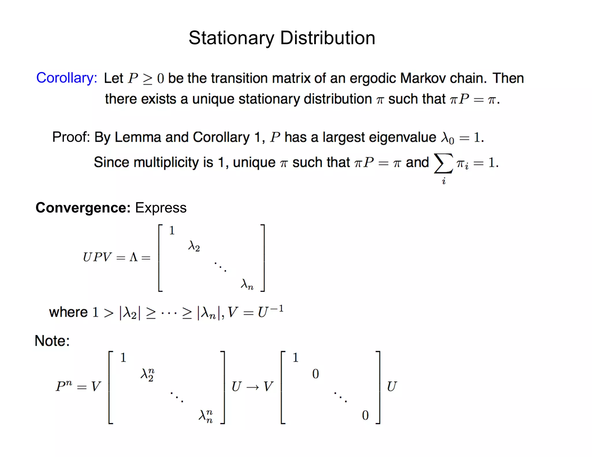
Stationary Distribution
Corollary:
Proof:
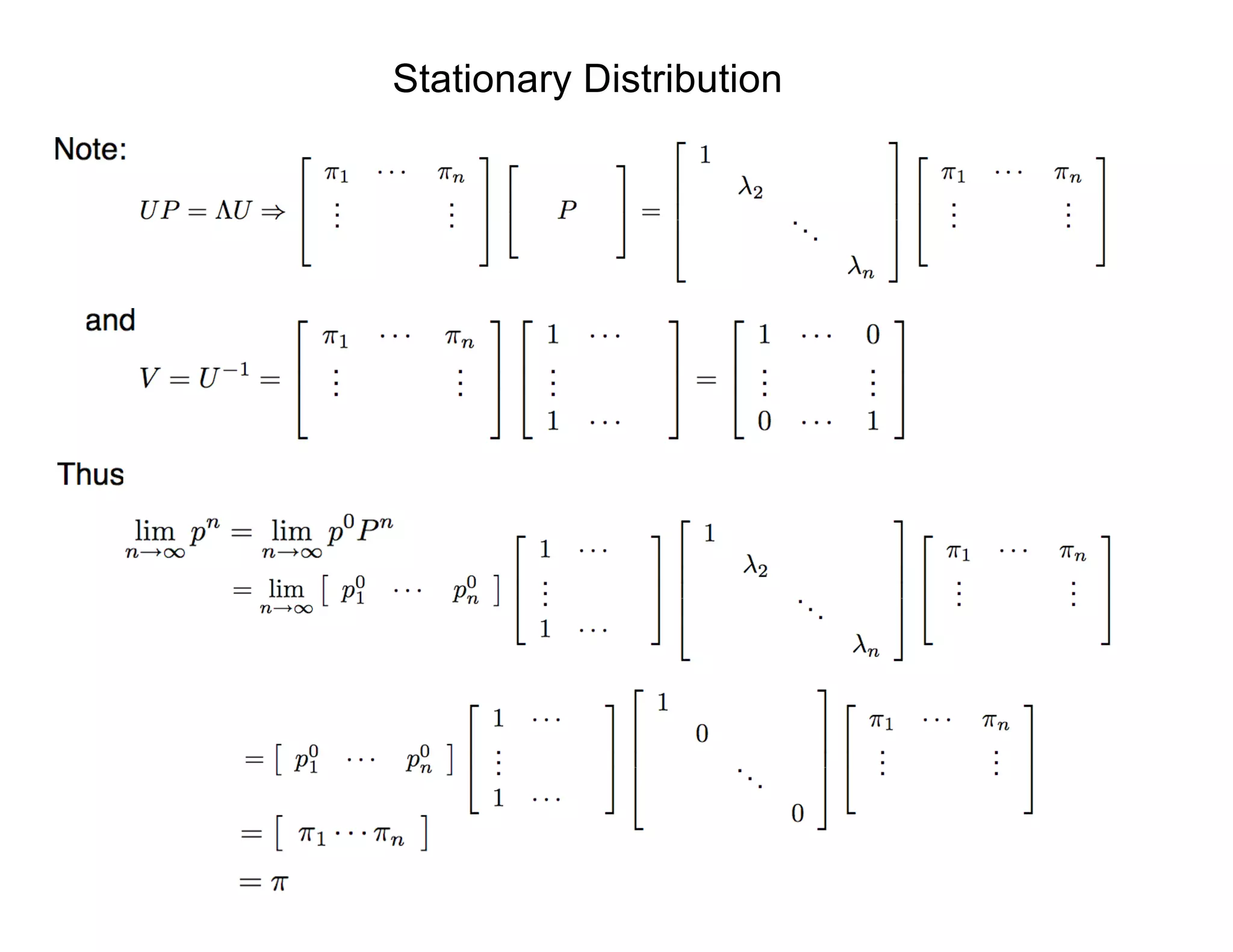
Convergence: Express
Stationary Distribution
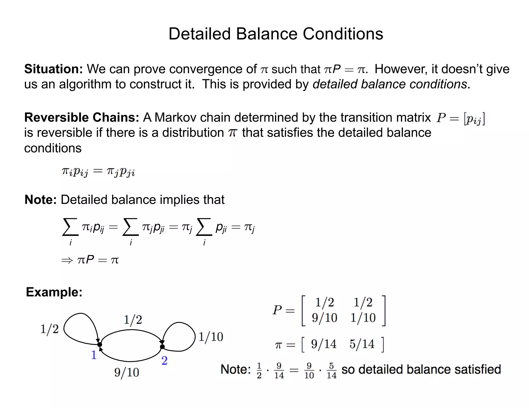
Detailed Balance Conditions
Reversible Chains: A Markov chain determined by the transition matrix
is reversible if there is a distribution that satisfies the detailed balance
conditions
Note: Detailed balance implies that
Example:
Situation: We can prove convergence of However, it doesn’t give
us an algorithm to construct it. This is provided by detailed balance conditions.
⇡ such that ⇡P = ⇡.
X
i
⇡i pij =
X
i
⇡j pji = ⇡j
X
i
pji = ⇡j
) ⇡P = ⇡
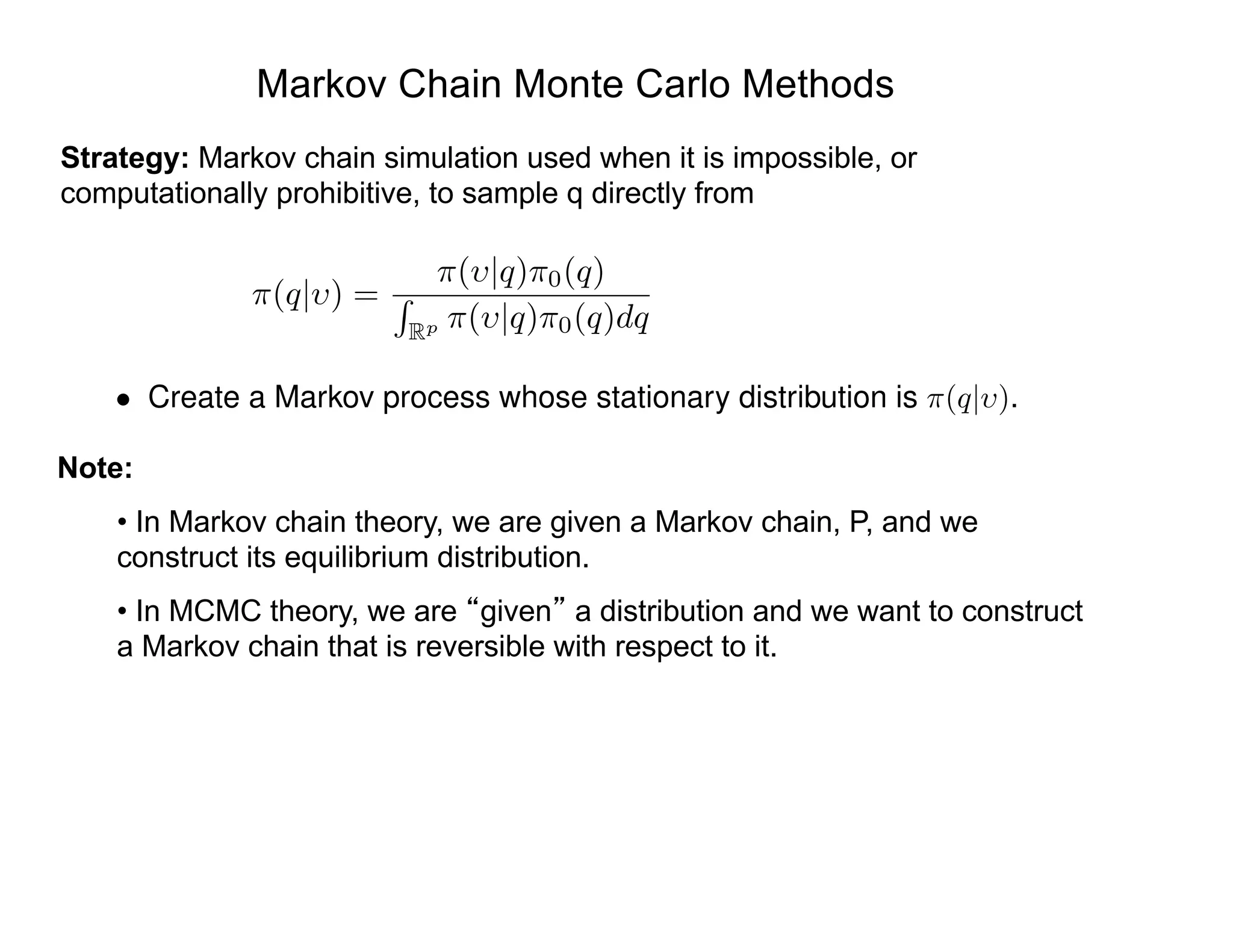
Markov Chain Monte Carlo Methods
Strategy: Markov chain simulation used when it is impossible, or
computationally prohibitive, to sample q directly from
Note:
• In Markov chain theory, we are given a Markov chain, P, and we
construct its equilibrium distribution.
• In MCMC theory, we are given a distribution and we want to construct
a Markov chain that is reversible with respect to it.
⇡(q| ) =
⇡( |q)⇡0(q)
R
Rp ⇡( |q)⇡0(q)dq
• Create a Markov process whose stationary distribution is ⇡(q| ).
Assumption: Assume that measurement errors are iid and
Model Calibration Problem
"i ⇠ N(0, 2
)
Likelihood:
⇡( |q) = L(q, | ) =
1
(2⇡ 2)n/2
e SSq/2 2
SSq =
nX
i=1
[ i fi(q)]
2
is the sum of squares error.
where
Markov Chain Monte Carlo Methods
Intuition:
|q)
* q*
qqk−1
SSq
qqk−1
(
q
Strategy:
of posterior distribution
• Compute r(q⇤
|qk-1
) = ⇡( |q⇤)⇡0(q⇤)
⇡( |qk-1)⇡0(qk-1)
⇤ If r > 1, accept with probability ↵ = 1
⇤ If r < 1, accept with probability ↵ = r
Consider flat prior ⇡0(q) = 1 and Gaussian observation model
⇡( |q) =
1
(2⇡ 2)n/2
e-SSq/2 2
SSq =
NX
i=1
[ i - f(ti , q)]2
• Sample values from proposal distribution J(q⇤
|qk-1
) that reflects geometry
Markov Chain Monte Carlo Methods
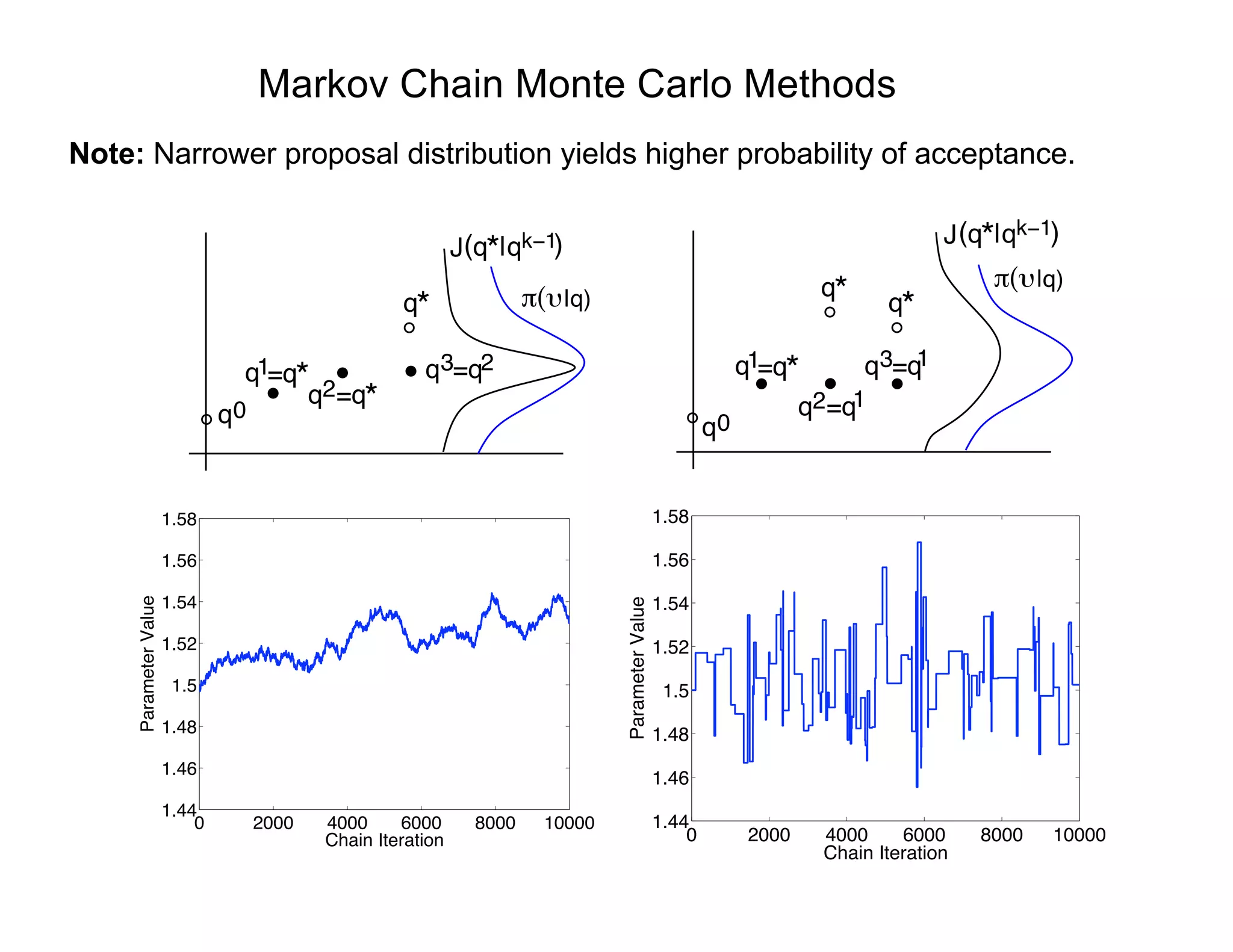
Note: Narrower proposal distribution yields higher probability of acceptance.
|q)*
=q*q1
=q*q2
=q2q3
q0
q*( |qk−1)J
(q
|q)
0
=q*q1
q2=q1
q3=q1
q* q*
q*( |qk−1)J
(
q
0 2000 4000 6000 8000 10000
1.44
1.46
1.48
1.5
1.52
1.54
1.56
1.58
Chain Iteration
ParameterValue
0 2000 4000 6000 8000 10000
1.44
1.46
1.48
1.5
1.52
1.54
1.56
1.58
Chain Iteration
ParameterValue
Proposal Distribution
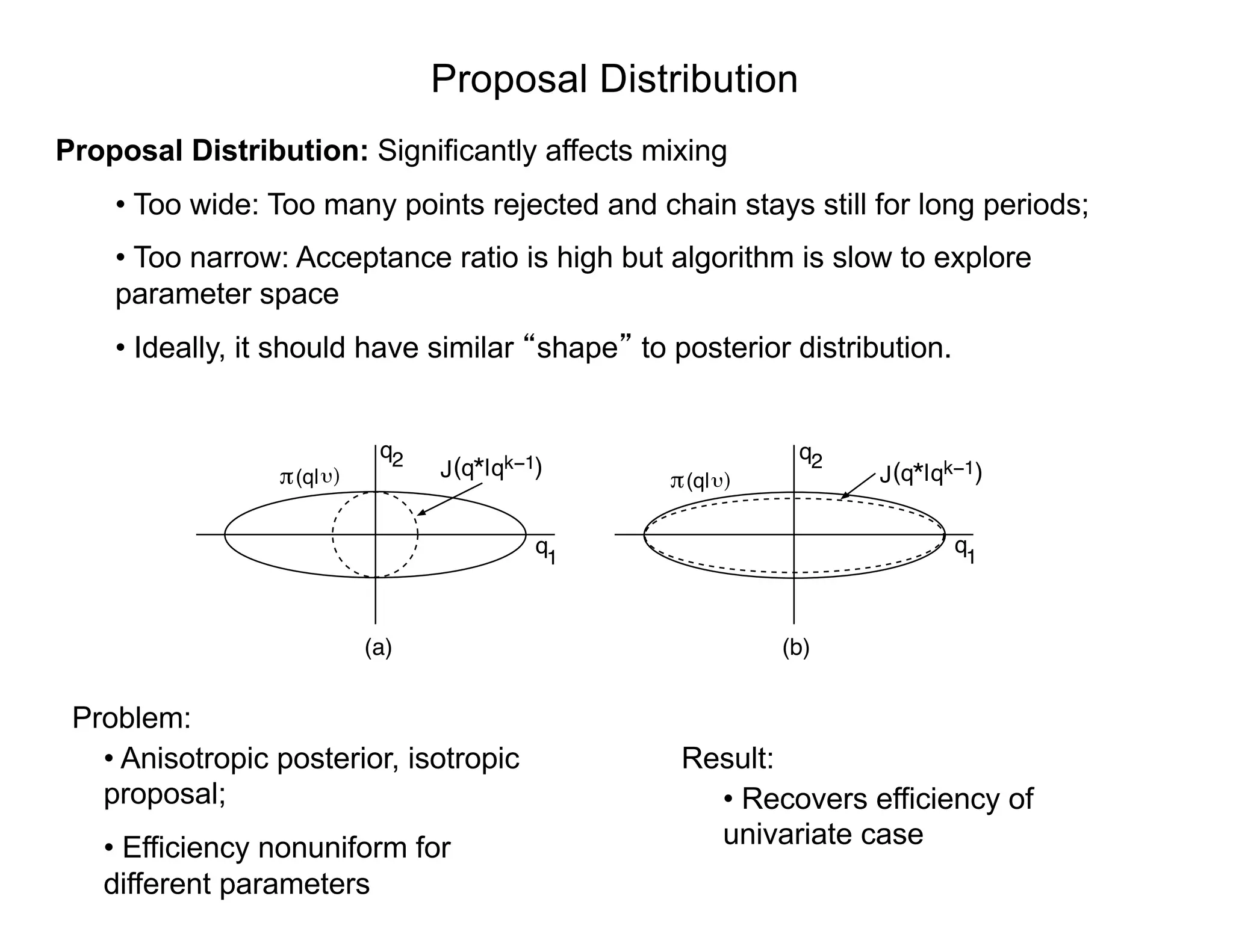
Proposal Distribution: Significantly affects mixing
• Too wide: Too many points rejected and chain stays still for long periods;
• Too narrow: Acceptance ratio is high but algorithm is slow to explore
parameter space
• Ideally, it should have similar shape to posterior distribution.
• Anisotropic posterior, isotropic
proposal;
• Efficiency nonuniform for
different parameters
Problem:
Result:
• Recovers efficiency of
univariate case
)
1
q2
q1
q2q*( |qk−1) q*( |qk−1)
(a) (b)
J J(q| (q| )
q
Proposal Distribution
Proposal Distribution: Two basic approaches
• Choose a fixed proposal function
o Independent Metropolis
• Random walk (local Metropolis)
o Two (of several) choices:
q⇤
= qk 1
+ Rz
(i) R = cI ) q⇤
⇠ N(qk 1
, cI)
(ii) R = chol(V ) ) q⇤
⇠ N(qk 1
, V )
where
)
1
q2
q1
q2q*( |qk−1) q*( |qk−1)
(a) (b)
J J(q| (q| )
q
V = 2
OLS
⇥
XT
(qOLS )X(qOLS )
⇤ 1
2
OLS =
1
n p
nX
i=1
[ i fi(qOLS )]
2
Sensitivity Matrix
Metropolis Algorithm
Metropolis Algorithm: [Metropolis and Ulam, 1949]
1. Initialization: Choose an initial parameter value q0
that satisfies ⇡(q0
| ) > 0.
2. For k = 1, · · · , M
(a) For z ⇠ N(0, 1), construct the candidate
q⇤
= qk 1
+ Rz
where R is the Cholesky decomposition of V or D. This ensures
that
q⇤
⇠ N(qk 1
, V ) or q⇤
⇠ N(qk 1
, D).
(b) Compute the ratio
r(q⇤
|qk 1
) =
⇡(q⇤
| )
⇡(qk 1| )
=
⇡( |q⇤
)⇡0(q⇤
)
⇡( |qk 1)⇡0(qk 1)
. (1)
(c) Set
qk
=
(
q⇤
, with probability ↵ = min(1, r)
qk 1
, else.
That is, we accept q⇤
with probability 1 if r 1 and we accept it with
probability r if r < 1.
Sampling Error Variance
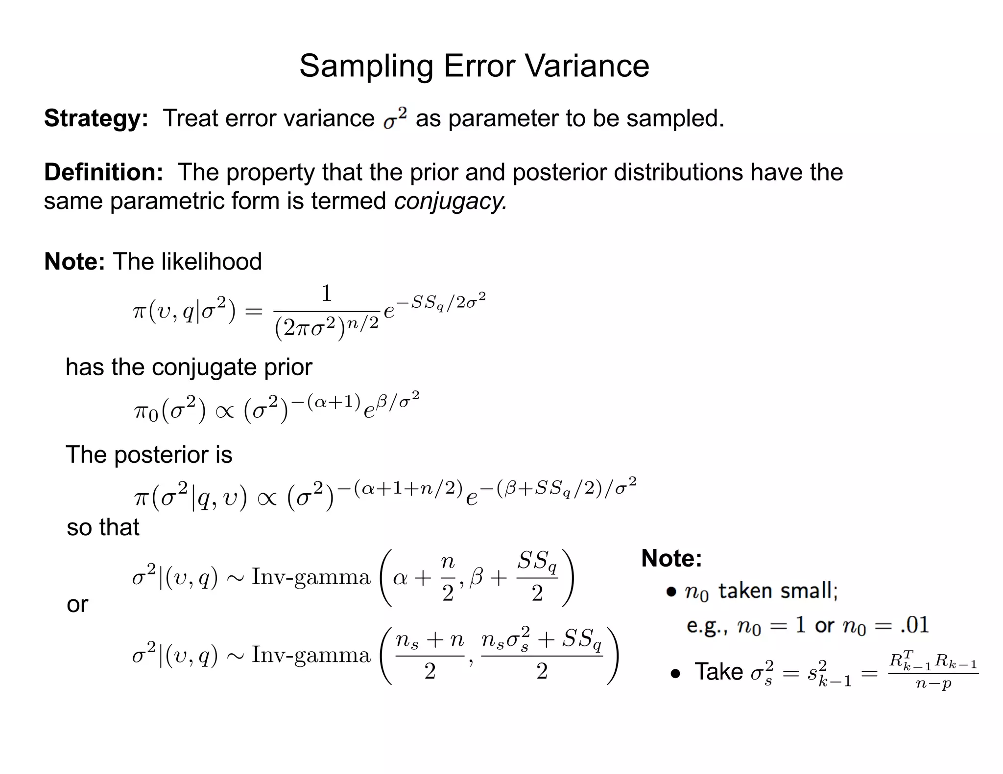
Strategy: Treat error variance as parameter to be sampled.
Definition: The property that the prior and posterior distributions have the
same parametric form is termed conjugacy.
Note: The likelihood
has the conjugate prior
The posterior is
so that
or
⇡0( 2
) / ( 2
) (↵+1)
e / 2
⇡( , q| 2
) =
1
(2⇡ 2)n/2
e SSq/2 2
⇡( 2
|q, ) / ( 2
) (↵+1+n/2)
e ( +SSq/2)/ 2
2
|( , q) ⇠ Inv-gamma
✓
↵ +
n
2
, +
SSq
2
◆
2
|( , q) ⇠ Inv-gamma
✓
ns + n
2
,
ns
2
s + SSq
2
◆
Note:
• Take 2
s = s2
k 1 =
RT
k 1Rk 1
n p
Delayed Rejection Adaptive Metropolis (DRAM)
Algorithm: [Haario et al., 2006] – MATLAB, PythonAlgorithm: [Haario et al., 2006] – MATLAB, Python, R
Example: Helmholtz energy
= ↵1P2
i + ↵11P4
i + "i
i = (Pi , q) + "i
"i ⇠ N(0, 2
)
Example: Helmholtz energy
1. Determine q0
= arg min
q
NX
i=1
[ i - (Pi , q)]2
]
Delayed Rejection Adaptive Metropolis (DRAM)
Algorithm: [Haario et al., 2006] – MATLAB, Python
-405 -400 -395 -390 -385 -380
α1
740
750
760
770
780
790
α
11
↵1
↵11
Algorithm: [Haario et al., 2006] – MATLAB, Python, R
Example: Helmholtz energy
= ↵1P2
i + ↵11P4
i + "i
i = (Pi , q) + "i
"i ⇠ N(0, 2
)
Recall: Covariance V incorporates geometry
Example: Helmholtz energy
q⇤
qk-1
1. Determine q0
= arg min
q
NX
i=1
[ i - (Pi , q)]2
]
2. For k = 1, ... , M
(a) Construct candidate q⇤
⇠ N(qk-1
, V)
34
Delayed Rejection Adaptive Metropolis (DRAM)
Algorithm: [Haario et al., 2006] – MATLAB, Python, R
1. Determine q0
= arg min
q
NX
i=1
[ i - (Pi , q)]2
]
2. For k = 1, ... , M
(a) Construct candidate q⇤
⇠ N(qk-1
, V)
(b) Compute likelihood
SSq⇤ =
NX
i=1
i - (Pi , q⇤
)]2
⇡( |q) =
1
(2⇡ 2)n/2
e-SSq/2 2
(c) Accept q⇤
with probability dictated by likelihood
Note:
• Delayed Rejection:
Shrink proposal:
• Adaptive Metropolis:
Update proposal as
samples are accepted
V
Random Walk Metropolis
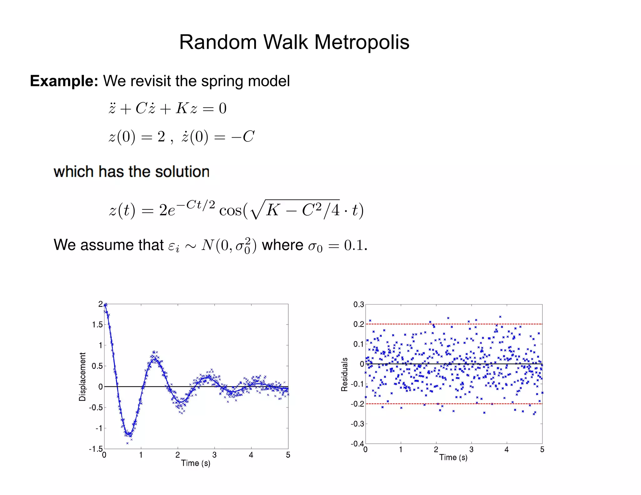
Example: We revisit the spring model
¨z + C ˙z + Kz = 0
z(0) = 2 , ˙z(0) = C
z(t) = 2e Ct/2
cos(
p
K C2/4 · t)
We assume that "i ⇠ N(0, 2
0) where 0 = 0.1.
Random Walk Metropolis
Case i: Take K =20.5 and Q = [C, 2
]
0 2000 4000 6000 8000 10000
1.4
1.42
1.44
1.46
1.48
1.5
1.52
1.54
Chain Iteration
DampingParameter
1.35 1.4 1.45 1.5 1.55 1.6
0
5
10
15
20
25
Damping Parameter C
Posterior
MCMC
Note: Kernel density estimator (KDE) used to construct density.
Random Walk Metropolis
Case ii: Take with andQ = [C, K, 2
] J(q⇤
|qk 1
) = N(qk 1
, V )
V =

0.000345 0.000268
0.000268 0.007071
0 2000 4000 6000 8000 10000
1.35
1.4
1.45
1.5
1.55
Chain Iteration
DampingParameterC
1.35 1.4 1.45 1.5 1.55
0
5
10
15
20
25
Damping Parameter C
0 2000 4000 6000 8000 10000
20.1
20.2
20.3
20.4
20.5
20.6
20.7
20.8
Chain Iteration
StiffnessParameterK
20 20.2 20.4 20.6 20.8 21
0
1
2
3
4
5
Stiffness Parameter K
Note:
2 C ⇡ 0.04
) 2
C ⇡ 0.4 ⇥ 10 3
) 2
K ⇡ 0.0081
2 K ⇡ 0.18
Random Walk Metropolis
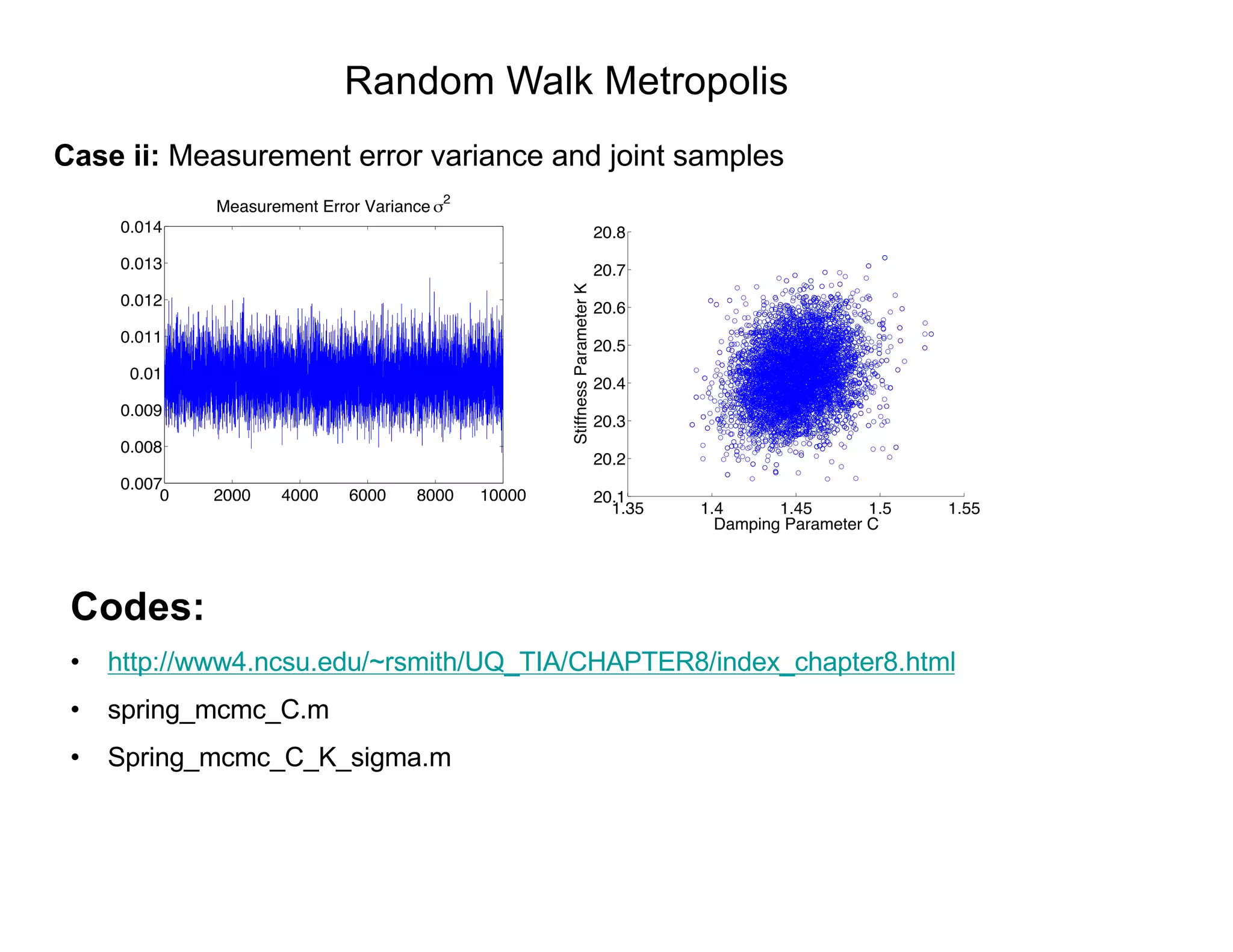
Case ii: Measurement error variance and joint samples
0 2000 4000 6000 8000 10000
0.007
0.008
0.009
0.01
0.011
0.012
0.013
0.014
Measurement Error Variance
2
1.35 1.4 1.45 1.5 1.55
20.1
20.2
20.3
20.4
20.5
20.6
20.7
20.8
Damping Parameter C
StiffnessParameterK
Codes:
• http://www4.ncsu.edu/~rsmith/UQ_TIA/CHAPTER8/index_chapter8.html
• spring_mcmc_C.m
• Spring_mcmc_C_K_sigma.m
Random Walk Metropolis
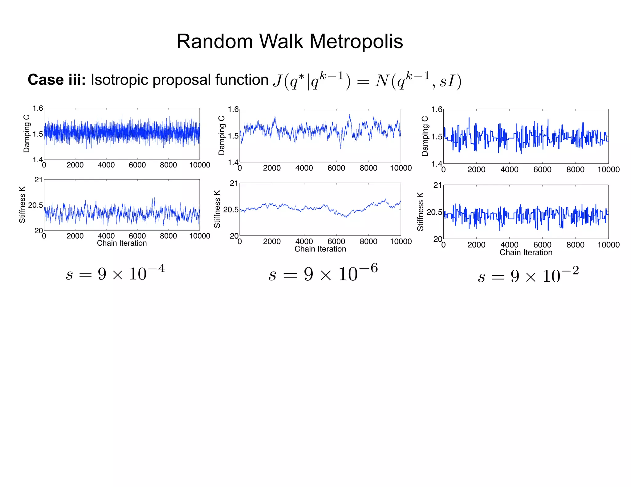
Case iii: Isotropic proposal function J(q⇤
|qk 1
) = N(qk 1
, sI)
0 2000 4000 6000 8000 10000
1.4
1.5
1.6
DampingC
0 2000 4000 6000 8000 10000
20
20.5
21
StiffnessK
Chain Iteration
0 2000 4000 6000 8000 10000
1.4
1.5
1.6
DampingC
0 2000 4000 6000 8000 10000
20
20.5
21
StiffnessK
Chain Iteration
0 2000 4000 6000 8000 10000
1.4
1.5
1.6
DampingC
0 2000 4000 6000 8000 10000
20
20.5
21
StiffnessK
Chain Iteration
s = 9 ⇥ 10 6
s = 9 ⇥ 10 4
s = 9 ⇥ 10 2
Stationary Distribution and Convergence Criteria
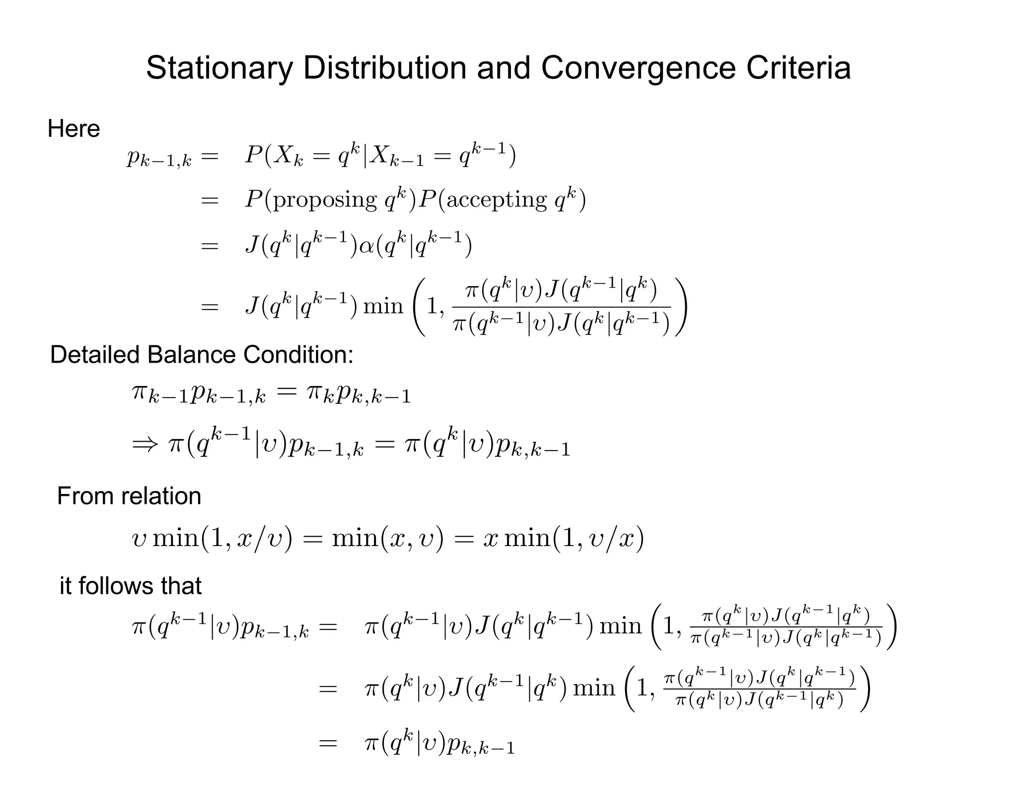
Here
Detailed Balance Condition:
pk 1,k = P(Xk = qk
|Xk 1 = qk 1
)
= P(proposing qk
)P(accepting qk
)
= J(qk
|qk 1
)↵(qk
|qk 1
)
= J(qk
|qk 1
) min
✓
1,
⇡(qk
| )J(qk 1
|qk
)
⇡(qk 1| )J(qk|qk 1)
◆
⇡k 1pk 1,k = ⇡kpk,k 1
) ⇡(qk 1
| )pk 1,k = ⇡(qk
| )pk,k 1
From relation
min(1, x/ ) = min(x, ) = x min(1, /x)
it follows that
⇡(qk 1
| )pk 1,k = ⇡(qk 1
| )J(qk
|qk 1
) min
⇣
1, ⇡(qk
| )J(qk 1
|qk
)
⇡(qk 1| )J(qk|qk 1)
⌘
= ⇡(qk
| )J(qk 1
|qk
) min
⇣
1, ⇡(qk 1
| )J(qk
|qk 1
)
⇡(qk| )J(qk 1|qk)
⌘
= ⇡(qk
| )pk,k 1
Delayed Rejection Adaptive Metropolis (DRAM)
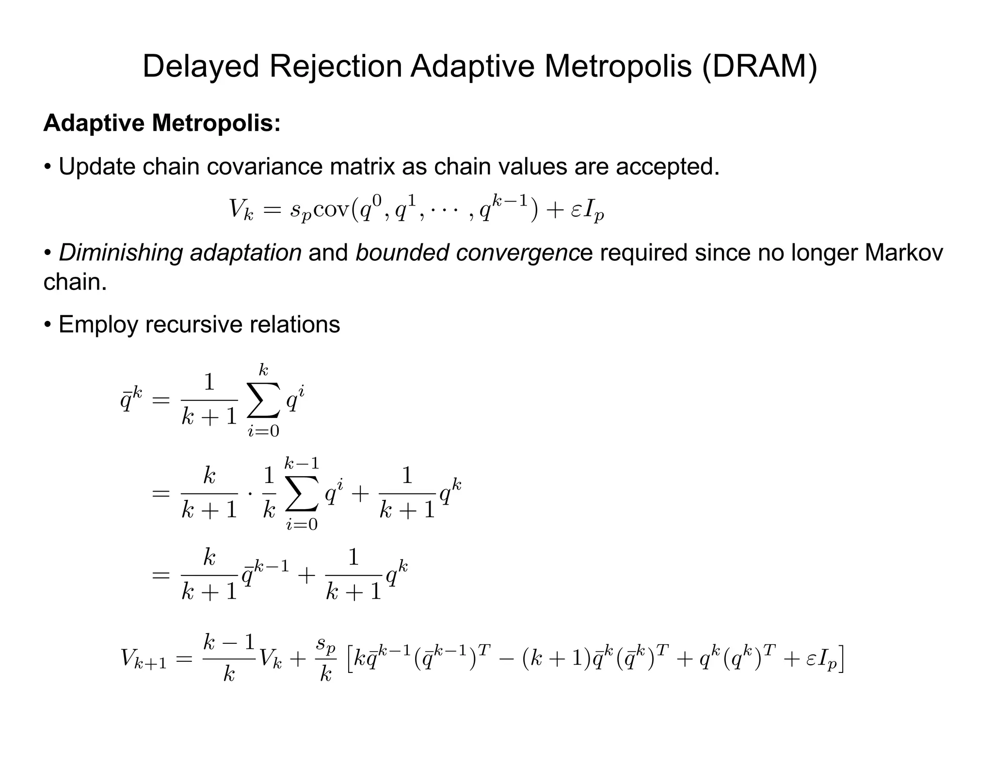
Adaptive Metropolis:
• Update chain covariance matrix as chain values are accepted.
• Diminishing adaptation and bounded convergence required since no longer Markov
chain.
• Employ recursive relations
Vk = spcov(q0
, q1
, · · · , qk 1
) + "Ip
Vk+1 =
k 1
k
Vk +
sp
k
⇥
k¯qk 1
(¯qk 1
)T
(k + 1)¯qk
(¯qk
)T
+ qk
(qk
)T
+ "Ip
⇤
¯qk
=
1
k + 1
kX
i=0
qi
=
k
k + 1
·
1
k
k 1X
i=0
qi
+
1
k + 1
qk
=
k
k + 1
¯qk 1
+
1
k + 1
qk
Delayed Rejection Adaptive Metropolis (DRAM)
Example: Heat model
d2
Ts
dx2
=
2(a + b)
ab
h
k
[Ts(x) Tamb]
dTs
dx
(0) =
k
,
dTs
dx
(L) =
h
k
[Tamb Ts(L)]
0 2000 4000 6000 8000 10000
1.85
1.9
1.95
2
x 10
!3
Chain Iteration
Parameterh
1.8 1.85 1.9 1.95 2
x 10
!3
0
0.5
1
1.5
2
2.5
3
x 10
4
Parameter h
0 2000 4000 6000 8000 10000
−19
−18.5
−18
−17.5
Chain Iteration
Parameter
−19.5 −19 −18.5 −18 −17.5
0
0.5
1
1.5
2
2.5
3
Parameter
Bayesian Analysis
= 0.2604
= 0.1552
h = 1.5450 ⇥ 10 5
Frequentist Analysis
h = 1.4482 ⇥ 10 5
= 0.1450
= 0.2504
Codes:
http://www4.ncsu.edu/~rsmith/UQ_TIA/CHA
PTER8/index_chapter8.html
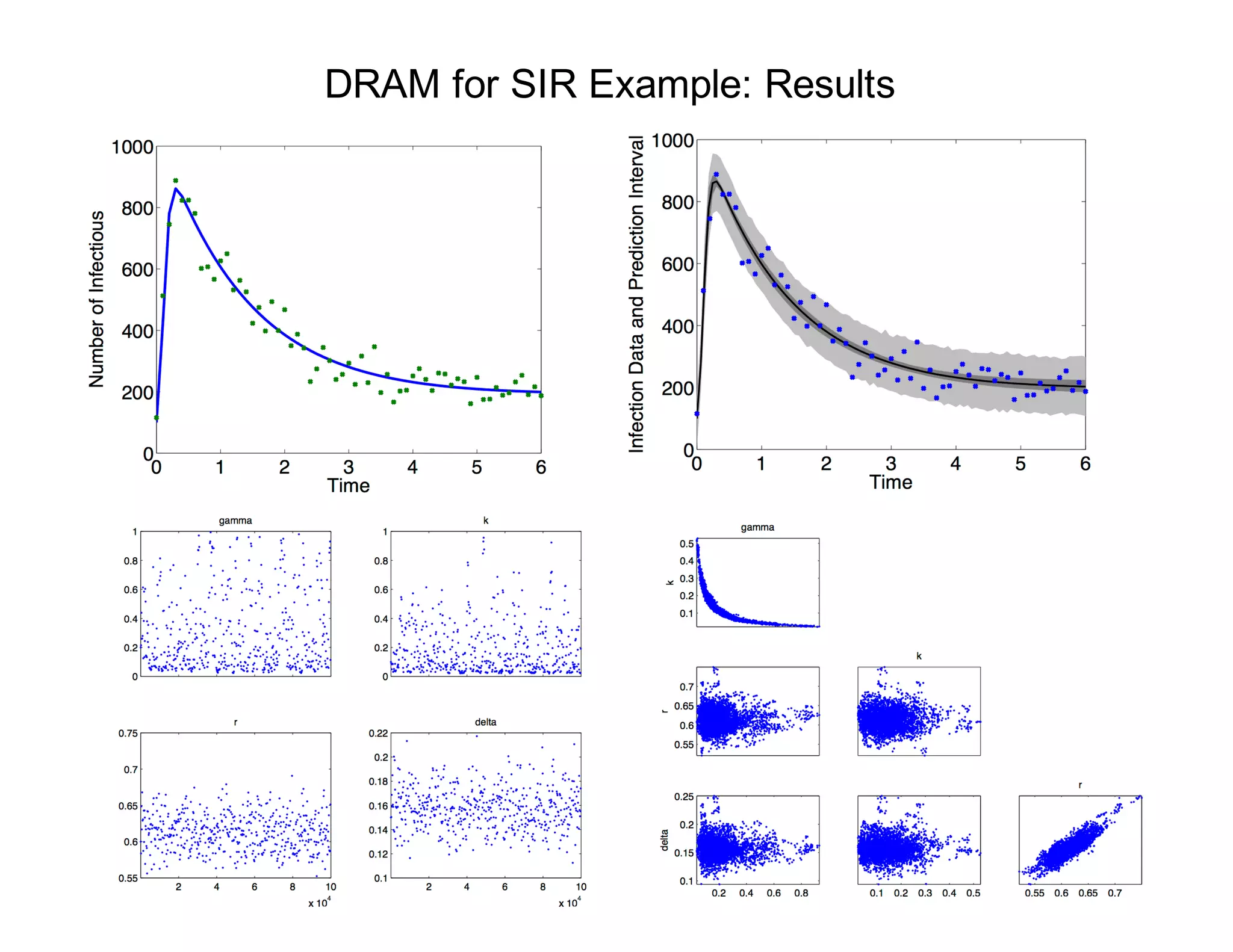
SIR Disease Example
SIR Model:
Susceptible
Infectious
Recovered
Note:
dS
dt
= N - S - kIS , S(0) = S0
dI
dt
= kIS - (r + )I , I(0) = I0
dR
dt
= rI - R , R(0) = R0
Parameter set q = [ , k, r, ] is not identifiable
Typical Realization:
49
DRAM for SIR Example: Results
50
SIR Disease Example
Codes: 4 parameter case
• SIR_dram.m
• SIR_rhs.m
• SIR_fun.m
• SIRss.m
• mcmcpredplot_custom.m
Project problem: Modify for 3 parameter case
• SIR_dram.m
• SIR_rhs.m
• SIR_fun.m
• SIRss.m
• mcmcpredplot_custom.m
Bayesian Inference: Advantages and Disadvantages
Advantages:
• Advantageous over frequentist inference when data is limited.
• Directly provides parameter densities, which can subsequently be propagated to
construct response uncertainties.
• Can be used to infer non-identifiable parameters if priors are tight.
• Provides natural framework for experimental design.
Disadvantages:
• More computationally intense than frequentist inference.
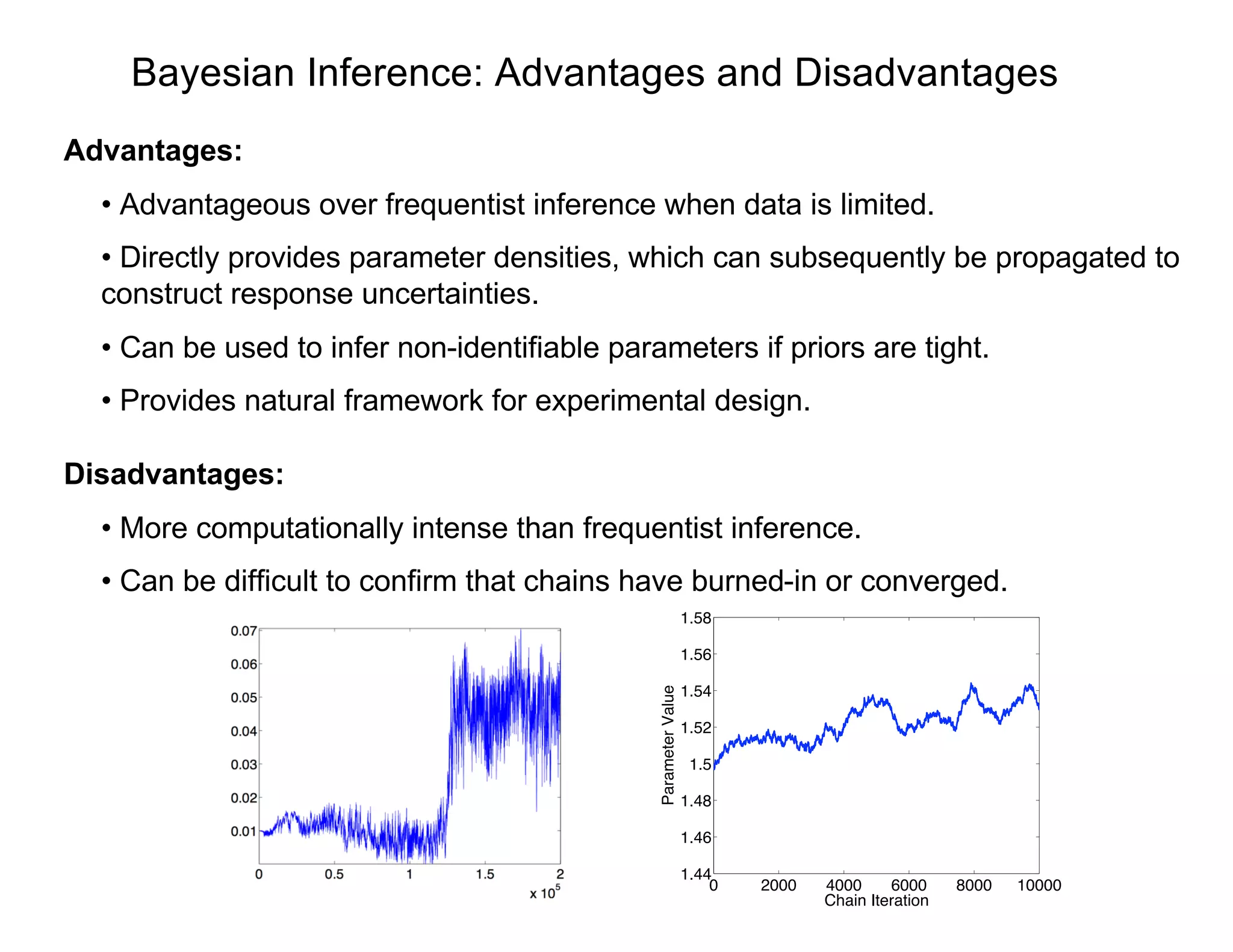
• Can be difficult to confirm that chains have burned-in or converged.
0 2000 4000 6000 8000 10000
1.44
1.46
1.48
1.5
1.52
1.54
1.56
1.58
Chain Iteration
ParameterValue
Delayed Rejection Adaptive Metropolis (DRAM)
Websites
•http://www4.ncsu.edu/~rsmith/UQ_TIA/CHAPTER8/index_chapter8.html
•http://helios.fmi.fi/~lainema/mcmc/
Examples
•Examples on using the toolbox for some statistical problems.
Delayed Rejection Adaptive Metropolis (DRAM)
We fit the Monod model
to observations
x (mg / L COD): 28 55 83 110 138 225 375
y (1 / h): 0.053 0.060 0.112 0.105 0.099 0.122 0.125
First clear some variables from possible previous runs.
clear data model options
Next, create a data structure for the observations and control variables. Typically one
could make a structure data that contains fields xdata and ydata.
data.xdata = [28 55 83 110 138 225 375]'; % x (mg / L COD)
data.ydata = [0.053 0.060 0.112 0.105 0.099 0.122 0.125]'; % y (1 / h)
Construct model
modelfun = @(x,theta) theta(1)*x./(theta(2)+x);
ssfun = @(theta,data) sum((data.ydata-modelfun(data.xdata,theta)).^2);
model.ssfun = ssfun;
model.sigma2 = 0.01^2;
y = ✓1
1
✓2 + 1
+ ✏ , ✏ ⇠ N(0, I 2
)
Delayed Rejection Adaptive Metropolis (DRAM)
Input parameters
params = {
{'theta1', tmin(1), 0}
{'theta2', tmin(2), 0} };
and set options
options.nsimu = 4000;
options.updatesigma = 1;
options.qcov = tcov;
Run code
[res,chain,s2chain] = mcmcrun(model,data,params,options);
Delayed Rejection Adaptive Metropolis (DRAM)
Plot results
figure(2); clf
mcmcplot(chain,[],res,'chainpanel');
figure(3); clf
mcmcplot(chain,[],res,'pairs');
Examples:
•Several available in MCMC_EXAMPLES
•ODE solver illustrated in algae example
Delayed Rejection Adaptive Metropolis (DRAM)
Construct credible and prediction intervals
figure(5); clf
out = mcmcpred(res,chain,[],x,modelfun);
mcmcpredplot(out);
hold on
plot(data.xdata,data.ydata,'s'); % add data points to the plot
xlabel('x [mg/L COD]');
ylabel('y [1/h]');
hold off
title('Predictive envelopes of the model')

2018 MUMS Fall Course - Bayesian inference for model calibration in UQ - Ralph Smith, October 16, 2018

  • 1.
    Bayesian Techniques forParameter Estimation
  • 2.
    Statistical Inference Goal: Thegoal in statistical inference is to make conclusions about a phenomenon based on observed data. Frequentist: Observations made in the past are analyzed with a specified model. Result is regarded as confidence about state of real world. • Probabilities defined as frequencies with which an event occurs if experiment is repeated several times. • Parameter Estimation: o Relies on estimators derived from different data sets and a specific sampling distribution. o Parameters may be unknown but are fixed and deterministic. Bayesian: Interpretation of probability is subjective and can be updated with new data. • Parameter Estimation: Parameters are considered to be random variables having associated densities.
  • 3.
    e Bayesian Inference: SimpleModel Example: Displacement-force relation (Hooke’s Law) Parameter: Stiffness E Strategy: Use model fit to data to update prior information Prior Information Information Provided by Model and Data Updated Information Non-normalized Bayes’ Relation: ModelData s(MPa) ⇡0(E) e- PN i=1[si -Eei ]2 /2 2 ⇡(E|s) ⇡(E|s) = e- PN i=1[si -Eei ]2 /2 2 ⇡0(E) si = Eei + "i , i = 1, ... , N "i ⇠ N(0, 2 )
  • 4.
    Bayesian Inference Bayes Relation:Specifies posterior in terms of likelihood and prior • Prior Distribution: Quantifies prior knowledge of parameter values • Likelihood: Probability of observing a data given set of parameter values. • Posterior Distribution: Conditional distribution of parameters given observed data. Problem: Can require high-dimensional integration • e.g., MFC Model: p = 20! • Solution: Sampling-based Markov Chain Monte Carlo (MCMC) algorithms. • Metropolis algorithms first used by nuclear physicists during Manhattan Project in 1940’s to understand particle movement underlying first atomic bomb. Posterior Distribution Normalization Constant Prior Distribution Likelihood: e- PN i=1[si -Eei ]2 /2 2 , q = E = [s1, ... , sN ] ⇡(q| ) = ⇡( |q)⇡0(q) R Rp ⇡( |q)⇡0(q)dq
  • 5.
    Bayesian Model Calibration BayesianModel Calibration: • Parameters assumed to be random variables Example: Coin Flip ⇡(q| ) = ⇡( |q)⇡0(q) R Rp ⇡( |q)⇡0(q)dq ⌥i(!) = ⇢ 0 , ! = T 1 , ! = H Likelihood: Posterior with Noninformative Prior: ⇡(q| ) = qN1 (1 q)N0 R 1 0 qN1 (1 q)N0 dq = (N + 1)! N0!N1! qN1 (1 q)N0 ⇡0(q) = 1 ⇡( |q) = NY i=1 q i (1 - q)1- i = qN1 (1 - q)N0 5
  • 6.
    Bayesian Inference Example: 1 Head,0 Tails 5 Heads, 9 Tails 49 Heads, 51 Tails Note:
  • 7.
    Bayesian Inference Example: Nowconsider Note: Poor informative prior incorrectly influences results for a long time. 50 Heads, 50 Tails5 Heads, 5 Tails ⇡0(q) = 1 p 2⇡ e (q µ)2 /2 2
  • 8.
    Likelihood: Assumption: Assume thatmeasurement errors are iid and Parameter Estimation Problem "i ⇠ N(0, 2 ) ⇡( |q) = L(q, | ) = 1 (2⇡ 2)n/2 e SSq/2 2 SSq = nX i=1 [ i fi(q)] 2 is the sum of squares error. where
  • 9.
    Parameter Estimation: Example Example:Consider the spring model ¨z + C ˙z + Kz = 0 z(0) = 2 , ˙z(0) = C z(t) = 2e Ct/2 cos( p K C2/4 · t) Note: Take K = 20.5, C0 = 1.5 Take K to be known and Q = C. We also assume that "i ⇠ N(0, 2 0) where 0 = 0.1.
  • 10.
    Parameter Estimation: Example OrdinaryLeast Squares: Here 1.4 1.45 1.5 1.55 1.6 0 5 10 15 20 25 Optimal C Density Contructed Sampling so that
  • 11.
    Parameter Estimation: Example BayesianInference: Employ the uniformed prior Note: • Slow even for one parameter. • Strategy: create Markov chain using random sampling so that created chain has the posterior distribution as its limiting (stationary) distribution. ⇡0(q) = [0,1)(q) Posterior Distribution: ⇡(q| ) = e SSq/2 2 0 R 1 0 e SS⇣ /2 2 0 d⇣ = 1 R 1 0 e (SS⇣ SSq)/2 2 0 d⇣ Midpoint formula: ⇡(q| ) ⇡ 1 P k e (SS⇣i SSq)wi/2 2 0 Issue: e SSqMAP ⇡ 3 ⇥ 10 113 1.4 1.45 1.5 1.55 1.6 0 5 10 15 20 25 Damping Parameter C Posterior Density Sampling Density
  • 12.
    Bayesian Model Calibration BayesianModel Calibration: •Parameters considered to be random variables with associated densities. Problem: •Often requires high dimensional integration; o e.g., p = 18 for MFC model o p = thousands to millions for some models Strategies: • Sampling methods • Sparse grid quadrature techniques ⇡(q| ) = ⇡( |q)⇡0(q) R Rp ⇡( |q)⇡0(q)dq
  • 13.
    Markov Chains Definition: Note: AMarkov chain is characterized by three components: a state space, an initial distribution, and a transition kernel. State Space: Initial Distribution: (Mass) Transition Probability: (Markov Kernel)
  • 14.
    Markov Chain Techniques MarkovChain: Sequence of events where current state depends only on last value. Baseball: • Assume that team which won last game has 70% chance of winning next game and 30% chance of losing next game. • Assume losing team wins 40% and loses 60% of next games. • Percentage of teams who win/lose next game given by • Question: does the following limit exist? States are S = {win,lose}. Initial state is p0 = [0.8, 0.2]. 0.7 win lose 0.4 0.3 0.6 p1 = [0.8 , 0.2]  0.7 0.3 0.4 0.6 = [0.64 , 0.36] pn = [0.8 , 0.2]  0.7 0.3 0.4 0.6 n
  • 15.
    Markov Chain Techniques BaseballExample: Solve constrained relation ⇡ = ⇡P , X ⇡i = 1 ) [⇡win , ⇡lose]  0.7 0.3 0.4 0.6 = [⇡win , ⇡lose] , ⇡win + ⇡lose = 1 to obtain ⇡ = [0.5714 , 0.4286]
  • 16.
    Markov Chain Techniques BaseballExample: Solve constrained relation ⇡ = ⇡P , X ⇡i = 1 ) [⇡win , ⇡lose]  0.7 0.3 0.4 0.6 = [⇡win , ⇡lose] , ⇡win + ⇡lose = 1 to obtain ⇡ = [0.5714 , 0.4286] Alternative: Iterate to compute solution n pn n pn n pn 0 [0.8000 , 0.2000] 4 [0.5733 , 0.4267] 8 [0.5714 , 0.4286] 1 [0.6400 , 0.3600] 5 [0.5720 , 0.4280] 9 [0.5714 , 0.4286] 2 [0.5920 , 0.4080] 6 [0.5716 , 0.4284] 10 [0.5714 , 0.4286] 3 [0.5776 , 0.4224] 7 [0.5715 , 0.4285] Notes: • Forms basis for Markov Chain Monte Carlo (MCMC) techniques • Goal: construct chains whose stationary distribution is the posterior density
  • 17.
    Irreducible Markov Chains Irreducible: ReducibleMarkov Chain: p1 p2 Note: Limiting distribution not unique if chain is reducible.
  • 18.
    Periodic Markov Chains Example: Periodicity:A Markov chain is periodic if parts of the state space are visited at regular intervals. The period k is defined as
  • 19.
    Stationary Distribution Theorem: Afinite, homogeneous Markov chain that is irreducible and aperiodic has a unique stationary distribution and the chain will converge in the sense of distributions from any initial distribution . Recurrence (Persistence): Example: State 3 is transient Ergodicity: A state is termed ergodic if it is aperiodic and recurrent. If all states of an irreducible Markov chain are ergodic, the chain is said to be ergodic.
  • 20.
  • 21.
  • 22.
  • 23.
  • 24.
    Detailed Balance Conditions ReversibleChains: A Markov chain determined by the transition matrix is reversible if there is a distribution that satisfies the detailed balance conditions Note: Detailed balance implies that Example: Situation: We can prove convergence of However, it doesn’t give us an algorithm to construct it. This is provided by detailed balance conditions. ⇡ such that ⇡P = ⇡. X i ⇡i pij = X i ⇡j pji = ⇡j X i pji = ⇡j ) ⇡P = ⇡
  • 25.
    Markov Chain MonteCarlo Methods Strategy: Markov chain simulation used when it is impossible, or computationally prohibitive, to sample q directly from Note: • In Markov chain theory, we are given a Markov chain, P, and we construct its equilibrium distribution. • In MCMC theory, we are given a distribution and we want to construct a Markov chain that is reversible with respect to it. ⇡(q| ) = ⇡( |q)⇡0(q) R Rp ⇡( |q)⇡0(q)dq • Create a Markov process whose stationary distribution is ⇡(q| ).
  • 26.
    Assumption: Assume thatmeasurement errors are iid and Model Calibration Problem "i ⇠ N(0, 2 ) Likelihood: ⇡( |q) = L(q, | ) = 1 (2⇡ 2)n/2 e SSq/2 2 SSq = nX i=1 [ i fi(q)] 2 is the sum of squares error. where
  • 27.
    Markov Chain MonteCarlo Methods Intuition: |q) * q* qqk−1 SSq qqk−1 ( q Strategy: of posterior distribution • Compute r(q⇤ |qk-1 ) = ⇡( |q⇤)⇡0(q⇤) ⇡( |qk-1)⇡0(qk-1) ⇤ If r > 1, accept with probability ↵ = 1 ⇤ If r < 1, accept with probability ↵ = r Consider flat prior ⇡0(q) = 1 and Gaussian observation model ⇡( |q) = 1 (2⇡ 2)n/2 e-SSq/2 2 SSq = NX i=1 [ i - f(ti , q)]2 • Sample values from proposal distribution J(q⇤ |qk-1 ) that reflects geometry
  • 28.
    Markov Chain MonteCarlo Methods Note: Narrower proposal distribution yields higher probability of acceptance. |q)* =q*q1 =q*q2 =q2q3 q0 q*( |qk−1)J (q |q) 0 =q*q1 q2=q1 q3=q1 q* q* q*( |qk−1)J ( q 0 2000 4000 6000 8000 10000 1.44 1.46 1.48 1.5 1.52 1.54 1.56 1.58 Chain Iteration ParameterValue 0 2000 4000 6000 8000 10000 1.44 1.46 1.48 1.5 1.52 1.54 1.56 1.58 Chain Iteration ParameterValue
  • 29.
    Proposal Distribution Proposal Distribution:Significantly affects mixing • Too wide: Too many points rejected and chain stays still for long periods; • Too narrow: Acceptance ratio is high but algorithm is slow to explore parameter space • Ideally, it should have similar shape to posterior distribution. • Anisotropic posterior, isotropic proposal; • Efficiency nonuniform for different parameters Problem: Result: • Recovers efficiency of univariate case ) 1 q2 q1 q2q*( |qk−1) q*( |qk−1) (a) (b) J J(q| (q| ) q
  • 30.
    Proposal Distribution Proposal Distribution:Two basic approaches • Choose a fixed proposal function o Independent Metropolis • Random walk (local Metropolis) o Two (of several) choices: q⇤ = qk 1 + Rz (i) R = cI ) q⇤ ⇠ N(qk 1 , cI) (ii) R = chol(V ) ) q⇤ ⇠ N(qk 1 , V ) where ) 1 q2 q1 q2q*( |qk−1) q*( |qk−1) (a) (b) J J(q| (q| ) q V = 2 OLS ⇥ XT (qOLS )X(qOLS ) ⇤ 1 2 OLS = 1 n p nX i=1 [ i fi(qOLS )] 2 Sensitivity Matrix
  • 31.
    Metropolis Algorithm Metropolis Algorithm:[Metropolis and Ulam, 1949] 1. Initialization: Choose an initial parameter value q0 that satisfies ⇡(q0 | ) > 0. 2. For k = 1, · · · , M (a) For z ⇠ N(0, 1), construct the candidate q⇤ = qk 1 + Rz where R is the Cholesky decomposition of V or D. This ensures that q⇤ ⇠ N(qk 1 , V ) or q⇤ ⇠ N(qk 1 , D). (b) Compute the ratio r(q⇤ |qk 1 ) = ⇡(q⇤ | ) ⇡(qk 1| ) = ⇡( |q⇤ )⇡0(q⇤ ) ⇡( |qk 1)⇡0(qk 1) . (1) (c) Set qk = ( q⇤ , with probability ↵ = min(1, r) qk 1 , else. That is, we accept q⇤ with probability 1 if r 1 and we accept it with probability r if r < 1.
  • 32.
    Sampling Error Variance Strategy:Treat error variance as parameter to be sampled. Definition: The property that the prior and posterior distributions have the same parametric form is termed conjugacy. Note: The likelihood has the conjugate prior The posterior is so that or ⇡0( 2 ) / ( 2 ) (↵+1) e / 2 ⇡( , q| 2 ) = 1 (2⇡ 2)n/2 e SSq/2 2 ⇡( 2 |q, ) / ( 2 ) (↵+1+n/2) e ( +SSq/2)/ 2 2 |( , q) ⇠ Inv-gamma ✓ ↵ + n 2 , + SSq 2 ◆ 2 |( , q) ⇠ Inv-gamma ✓ ns + n 2 , ns 2 s + SSq 2 ◆ Note: • Take 2 s = s2 k 1 = RT k 1Rk 1 n p
  • 33.
    Delayed Rejection AdaptiveMetropolis (DRAM) Algorithm: [Haario et al., 2006] – MATLAB, PythonAlgorithm: [Haario et al., 2006] – MATLAB, Python, R Example: Helmholtz energy = ↵1P2 i + ↵11P4 i + "i i = (Pi , q) + "i "i ⇠ N(0, 2 ) Example: Helmholtz energy 1. Determine q0 = arg min q NX i=1 [ i - (Pi , q)]2 ]
  • 34.
    Delayed Rejection AdaptiveMetropolis (DRAM) Algorithm: [Haario et al., 2006] – MATLAB, Python -405 -400 -395 -390 -385 -380 α1 740 750 760 770 780 790 α 11 ↵1 ↵11 Algorithm: [Haario et al., 2006] – MATLAB, Python, R Example: Helmholtz energy = ↵1P2 i + ↵11P4 i + "i i = (Pi , q) + "i "i ⇠ N(0, 2 ) Recall: Covariance V incorporates geometry Example: Helmholtz energy q⇤ qk-1 1. Determine q0 = arg min q NX i=1 [ i - (Pi , q)]2 ] 2. For k = 1, ... , M (a) Construct candidate q⇤ ⇠ N(qk-1 , V) 34
  • 35.
    Delayed Rejection AdaptiveMetropolis (DRAM) Algorithm: [Haario et al., 2006] – MATLAB, Python, R 1. Determine q0 = arg min q NX i=1 [ i - (Pi , q)]2 ] 2. For k = 1, ... , M (a) Construct candidate q⇤ ⇠ N(qk-1 , V) (b) Compute likelihood SSq⇤ = NX i=1 i - (Pi , q⇤ )]2 ⇡( |q) = 1 (2⇡ 2)n/2 e-SSq/2 2 (c) Accept q⇤ with probability dictated by likelihood
  • 36.
    Delayed Rejection AdaptiveMetropolis (DRAM) Algorithm: [Haario et al., 2006] – MATLAB, Python, R 1. Determine q0 = arg min q NX i=1 [ i - (Pi , q)]2 ] 2. For k = 1, ... , M (a) Construct candidate q⇤ ⇠ N(qk-1 , V) (b) Compute likelihood SSq⇤ = NX i=1 i - (Pi , q⇤ )]2 ⇡( |q) = 1 (2⇡ 2)n/2 e-SSq/2 2 (c) Accept q⇤ with probability dictated by likelihood
  • 37.
    Delayed Rejection AdaptiveMetropolis (DRAM) Algorithm: [Haario et al., 2006] – MATLAB, Python, R 1. Determine q0 = arg min q NX i=1 [ i - (Pi , q)]2 ] 2. For k = 1, ... , M (a) Construct candidate q⇤ ⇠ N(qk-1 , V) (b) Compute likelihood SSq⇤ = NX i=1 i - (Pi , q⇤ )]2 ⇡( |q) = 1 (2⇡ 2)n/2 e-SSq/2 2 (c) Accept q⇤ with probability dictated by likelihood
  • 38.
    Delayed Rejection AdaptiveMetropolis (DRAM) Algorithm: [Haario et al., 2006] – MATLAB, Python, R 1. Determine q0 = arg min q NX i=1 [ i - (Pi , q)]2 ] 2. For k = 1, ... , M (a) Construct candidate q⇤ ⇠ N(qk-1 , V) (b) Compute likelihood SSq⇤ = NX i=1 i - (Pi , q⇤ )]2 ⇡( |q) = 1 (2⇡ 2)n/2 e-SSq/2 2 (c) Accept q⇤ with probability dictated by likelihood
  • 39.
    Delayed Rejection AdaptiveMetropolis (DRAM) Algorithm: [Haario et al., 2006] – MATLAB, Python, R 1. Determine q0 = arg min q NX i=1 [ i - (Pi , q)]2 ] 2. For k = 1, ... , M (a) Construct candidate q⇤ ⇠ N(qk-1 , V) (b) Compute likelihood SSq⇤ = NX i=1 i - (Pi , q⇤ )]2 ⇡( |q) = 1 (2⇡ 2)n/2 e-SSq/2 2 (c) Accept q⇤ with probability dictated by likelihood Note: • Delayed Rejection: Shrink proposal: • Adaptive Metropolis: Update proposal as samples are accepted V
  • 40.
    Random Walk Metropolis Example:We revisit the spring model ¨z + C ˙z + Kz = 0 z(0) = 2 , ˙z(0) = C z(t) = 2e Ct/2 cos( p K C2/4 · t) We assume that "i ⇠ N(0, 2 0) where 0 = 0.1.
  • 41.
    Random Walk Metropolis Casei: Take K =20.5 and Q = [C, 2 ] 0 2000 4000 6000 8000 10000 1.4 1.42 1.44 1.46 1.48 1.5 1.52 1.54 Chain Iteration DampingParameter 1.35 1.4 1.45 1.5 1.55 1.6 0 5 10 15 20 25 Damping Parameter C Posterior MCMC Note: Kernel density estimator (KDE) used to construct density.
  • 42.
    Random Walk Metropolis Caseii: Take with andQ = [C, K, 2 ] J(q⇤ |qk 1 ) = N(qk 1 , V ) V =  0.000345 0.000268 0.000268 0.007071 0 2000 4000 6000 8000 10000 1.35 1.4 1.45 1.5 1.55 Chain Iteration DampingParameterC 1.35 1.4 1.45 1.5 1.55 0 5 10 15 20 25 Damping Parameter C 0 2000 4000 6000 8000 10000 20.1 20.2 20.3 20.4 20.5 20.6 20.7 20.8 Chain Iteration StiffnessParameterK 20 20.2 20.4 20.6 20.8 21 0 1 2 3 4 5 Stiffness Parameter K Note: 2 C ⇡ 0.04 ) 2 C ⇡ 0.4 ⇥ 10 3 ) 2 K ⇡ 0.0081 2 K ⇡ 0.18
  • 43.
    Random Walk Metropolis Caseii: Measurement error variance and joint samples 0 2000 4000 6000 8000 10000 0.007 0.008 0.009 0.01 0.011 0.012 0.013 0.014 Measurement Error Variance 2 1.35 1.4 1.45 1.5 1.55 20.1 20.2 20.3 20.4 20.5 20.6 20.7 20.8 Damping Parameter C StiffnessParameterK Codes: • http://www4.ncsu.edu/~rsmith/UQ_TIA/CHAPTER8/index_chapter8.html • spring_mcmc_C.m • Spring_mcmc_C_K_sigma.m
  • 44.
    Random Walk Metropolis Caseiii: Isotropic proposal function J(q⇤ |qk 1 ) = N(qk 1 , sI) 0 2000 4000 6000 8000 10000 1.4 1.5 1.6 DampingC 0 2000 4000 6000 8000 10000 20 20.5 21 StiffnessK Chain Iteration 0 2000 4000 6000 8000 10000 1.4 1.5 1.6 DampingC 0 2000 4000 6000 8000 10000 20 20.5 21 StiffnessK Chain Iteration 0 2000 4000 6000 8000 10000 1.4 1.5 1.6 DampingC 0 2000 4000 6000 8000 10000 20 20.5 21 StiffnessK Chain Iteration s = 9 ⇥ 10 6 s = 9 ⇥ 10 4 s = 9 ⇥ 10 2
  • 45.
    Stationary Distribution andConvergence Criteria Here Detailed Balance Condition: pk 1,k = P(Xk = qk |Xk 1 = qk 1 ) = P(proposing qk )P(accepting qk ) = J(qk |qk 1 )↵(qk |qk 1 ) = J(qk |qk 1 ) min ✓ 1, ⇡(qk | )J(qk 1 |qk ) ⇡(qk 1| )J(qk|qk 1) ◆ ⇡k 1pk 1,k = ⇡kpk,k 1 ) ⇡(qk 1 | )pk 1,k = ⇡(qk | )pk,k 1 From relation min(1, x/ ) = min(x, ) = x min(1, /x) it follows that ⇡(qk 1 | )pk 1,k = ⇡(qk 1 | )J(qk |qk 1 ) min ⇣ 1, ⇡(qk | )J(qk 1 |qk ) ⇡(qk 1| )J(qk|qk 1) ⌘ = ⇡(qk | )J(qk 1 |qk ) min ⇣ 1, ⇡(qk 1 | )J(qk |qk 1 ) ⇡(qk| )J(qk 1|qk) ⌘ = ⇡(qk | )pk,k 1
  • 46.
    Delayed Rejection AdaptiveMetropolis (DRAM) Adaptive Metropolis: • Update chain covariance matrix as chain values are accepted. • Diminishing adaptation and bounded convergence required since no longer Markov chain. • Employ recursive relations Vk = spcov(q0 , q1 , · · · , qk 1 ) + "Ip Vk+1 = k 1 k Vk + sp k ⇥ k¯qk 1 (¯qk 1 )T (k + 1)¯qk (¯qk )T + qk (qk )T + "Ip ⇤ ¯qk = 1 k + 1 kX i=0 qi = k k + 1 · 1 k k 1X i=0 qi + 1 k + 1 qk = k k + 1 ¯qk 1 + 1 k + 1 qk
  • 47.
    Delayed Rejection AdaptiveMetropolis (DRAM) Example: Heat model d2 Ts dx2 = 2(a + b) ab h k [Ts(x) Tamb] dTs dx (0) = k , dTs dx (L) = h k [Tamb Ts(L)] 0 2000 4000 6000 8000 10000 1.85 1.9 1.95 2 x 10 !3 Chain Iteration Parameterh 1.8 1.85 1.9 1.95 2 x 10 !3 0 0.5 1 1.5 2 2.5 3 x 10 4 Parameter h 0 2000 4000 6000 8000 10000 −19 −18.5 −18 −17.5 Chain Iteration Parameter −19.5 −19 −18.5 −18 −17.5 0 0.5 1 1.5 2 2.5 3 Parameter Bayesian Analysis = 0.2604 = 0.1552 h = 1.5450 ⇥ 10 5 Frequentist Analysis h = 1.4482 ⇥ 10 5 = 0.1450 = 0.2504 Codes: http://www4.ncsu.edu/~rsmith/UQ_TIA/CHA PTER8/index_chapter8.html
  • 48.
    SIR Disease Example SIRModel: Susceptible Infectious Recovered Note: dS dt = N - S - kIS , S(0) = S0 dI dt = kIS - (r + )I , I(0) = I0 dR dt = rI - R , R(0) = R0 Parameter set q = [ , k, r, ] is not identifiable Typical Realization:
  • 49.
    49 DRAM for SIRExample: Results
  • 50.
    50 SIR Disease Example Codes:4 parameter case • SIR_dram.m • SIR_rhs.m • SIR_fun.m • SIRss.m • mcmcpredplot_custom.m Project problem: Modify for 3 parameter case • SIR_dram.m • SIR_rhs.m • SIR_fun.m • SIRss.m • mcmcpredplot_custom.m
  • 51.
    Bayesian Inference: Advantagesand Disadvantages Advantages: • Advantageous over frequentist inference when data is limited. • Directly provides parameter densities, which can subsequently be propagated to construct response uncertainties. • Can be used to infer non-identifiable parameters if priors are tight. • Provides natural framework for experimental design. Disadvantages: • More computationally intense than frequentist inference. • Can be difficult to confirm that chains have burned-in or converged. 0 2000 4000 6000 8000 10000 1.44 1.46 1.48 1.5 1.52 1.54 1.56 1.58 Chain Iteration ParameterValue
  • 52.
    Delayed Rejection AdaptiveMetropolis (DRAM) Websites •http://www4.ncsu.edu/~rsmith/UQ_TIA/CHAPTER8/index_chapter8.html •http://helios.fmi.fi/~lainema/mcmc/ Examples •Examples on using the toolbox for some statistical problems.
  • 53.
    Delayed Rejection AdaptiveMetropolis (DRAM) We fit the Monod model to observations x (mg / L COD): 28 55 83 110 138 225 375 y (1 / h): 0.053 0.060 0.112 0.105 0.099 0.122 0.125 First clear some variables from possible previous runs. clear data model options Next, create a data structure for the observations and control variables. Typically one could make a structure data that contains fields xdata and ydata. data.xdata = [28 55 83 110 138 225 375]'; % x (mg / L COD) data.ydata = [0.053 0.060 0.112 0.105 0.099 0.122 0.125]'; % y (1 / h) Construct model modelfun = @(x,theta) theta(1)*x./(theta(2)+x); ssfun = @(theta,data) sum((data.ydata-modelfun(data.xdata,theta)).^2); model.ssfun = ssfun; model.sigma2 = 0.01^2; y = ✓1 1 ✓2 + 1 + ✏ , ✏ ⇠ N(0, I 2 )
  • 54.
    Delayed Rejection AdaptiveMetropolis (DRAM) Input parameters params = { {'theta1', tmin(1), 0} {'theta2', tmin(2), 0} }; and set options options.nsimu = 4000; options.updatesigma = 1; options.qcov = tcov; Run code [res,chain,s2chain] = mcmcrun(model,data,params,options);
  • 55.
    Delayed Rejection AdaptiveMetropolis (DRAM) Plot results figure(2); clf mcmcplot(chain,[],res,'chainpanel'); figure(3); clf mcmcplot(chain,[],res,'pairs'); Examples: •Several available in MCMC_EXAMPLES •ODE solver illustrated in algae example
  • 56.
    Delayed Rejection AdaptiveMetropolis (DRAM) Construct credible and prediction intervals figure(5); clf out = mcmcpred(res,chain,[],x,modelfun); mcmcpredplot(out); hold on plot(data.xdata,data.ydata,'s'); % add data points to the plot xlabel('x [mg/L COD]'); ylabel('y [1/h]'); hold off title('Predictive envelopes of the model')