Download as PDF, PPTX
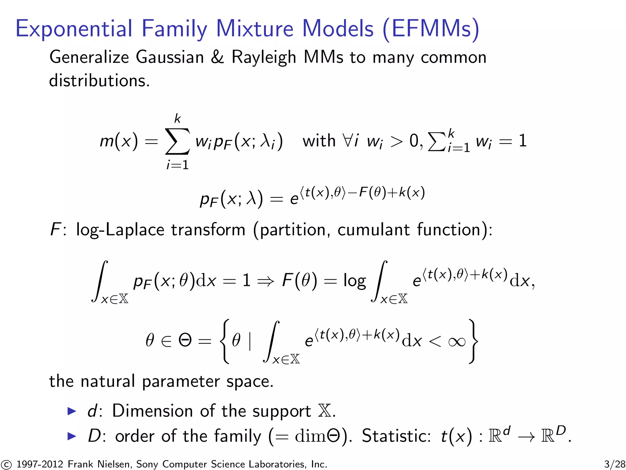
![Statistical mixtures: Rayleigh MMs [7, 5]
IntraVascular UltraSound (IVUS) imaging:
Rayleigh distribution:
p(x; ) = x
2 e− x2
22
x 2 R+ = X
d = 1 (univariate)
D = 1 (order 1)
= − 1
22
= (−1, 0)
F() = −log(−2)
t(x) = x2
k(x) = log x
(Weibull k = 2)
Coronary plaques: fibrotic tissues, calcified tissues, lipidic tissues
Rayleigh Mixture Models (RMMs):
for segmentation and classification tasks
c 1997-2012 Frank Nielsen, Sony Computer Science Laboratories, Inc. 4/28](https://image.slidesharecdn.com/kmle-talk-icassp2012-140902021340-phpapp02/75/k-MLE-A-fast-algorithm-for-learning-statistical-mixture-models-4-2048.jpg)
![Statistical mixtures: Gaussian MMs [3, 5]
Gaussian mixture models (GMMs).
Color image interpreted as a 5D xyRGB point set.
Gaussian distribution p(x; μ,):
1
(2)
d
2p||
e−1
2D−1 (x−μ,x−μ)
Squared Mahalanobis distance:
DQ(x, y) = (x − y)TQ(x − y)
x 2 Rd = X
d (multivariate)
D = d(d+3)
2 (order)
= (−1μ, 1
2−1) = (v , M)
= R × Sd+
+
F() = 1
v −1
4 T
M v − 1
2 log |M| +
d
2 log
t(x) = (x,−xxT )
k(x) = 0
c 1997-2012 Frank Nielsen, Sony Computer Science Laboratories, Inc. 5/28](https://image.slidesharecdn.com/kmle-talk-icassp2012-140902021340-phpapp02/75/k-MLE-A-fast-algorithm-for-learning-statistical-mixture-models-5-2048.jpg)
![Sampling from a Gaussian Mixture Model (GMM)
To sample a variate x from a GMM:
I Choose a component l according to the weight distribution
w1, ...,wk ,
I Draw a variate x according to N(μl ,l ).
Doubly stochastic process:
1. throw a (biased) dice with k faces to choose the component:
l Multinomial(w1, ...,wk )
(Multinomial distribution belongs also to the exponential
families.)
2. then draw at random a variate x from the l -th component
x Normal(μl ,l )
x = μ + Cz with Cholesky: = CCT and z = [z1 ... zd ]T
standard normal random variate: zi = p−2 log U1 cos(2U2)
c 1997-2012 Frank Nielsen, Sony Computer Science Laboratories, Inc. 6/28](https://image.slidesharecdn.com/kmle-talk-icassp2012-140902021340-phpapp02/75/k-MLE-A-fast-algorithm-for-learning-statistical-mixture-models-6-2048.jpg)

![Distance between exponential families: Relative entropy
I Distance between features (e.g., GMMs)
I Kullback-Leibler divergence (cross-entropy minus entropy):
KL(P : Q) =
Z
p(x) log
p(x)
q(x)
dx 0
=
Z
p(x) log
1
q(x)
dx
| {z }
H×(P:Q)
−
Z
p(x) log
1
p(x)
dx
| {z }
H(p)=H×(P:P)
= F(Q) − F(P) − hQ − P,rF(P)i
= BF (Q : P)
Bregman divergence BF defined for a strictly convex and
differentiable function (up to some affine terms).
I Proof KL(P : Q) = BF (Q : P) follows from
X EF () =) E[t(X)] = rF()
c 1997-2012 Frank Nielsen, Sony Computer Science Laboratories, Inc. 8/28](https://image.slidesharecdn.com/kmle-talk-icassp2012-140902021340-phpapp02/75/k-MLE-A-fast-algorithm-for-learning-statistical-mixture-models-8-2048.jpg)
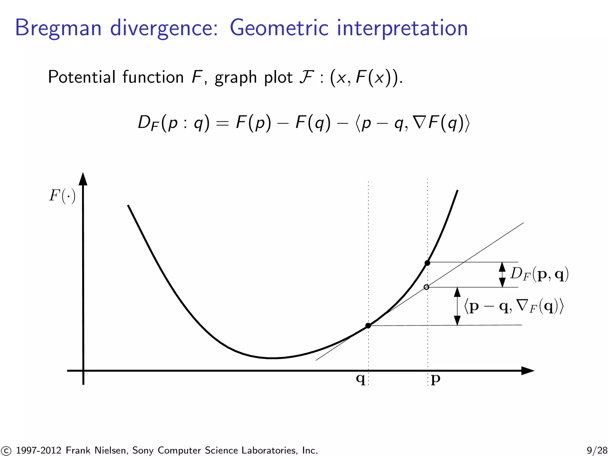
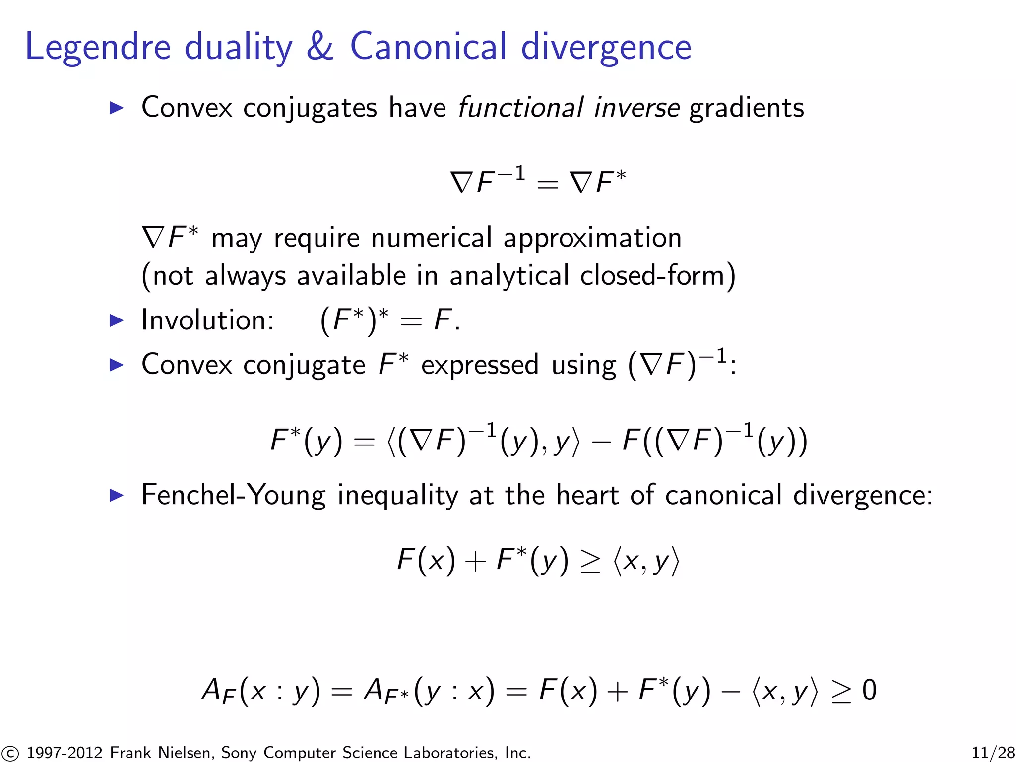
![Dual Bregman divergences canonical divergence [6]
KL(P : Q) = EP
log
p(x)
q(x)
0
= BF (Q : P) = BF(P : Q)
= F(Q) + F(P) − hQ, Pi
= AF (Q : P) = AF(P : Q)
with Q (natural parameterization) and P = EP[t(X)] = rF(P)
(moment parameterization).
c 1997-2012 Frank Nielsen, Sony Computer Science Laboratories, Inc. 12/28](https://image.slidesharecdn.com/kmle-talk-icassp2012-140902021340-phpapp02/75/k-MLE-A-fast-algorithm-for-learning-statistical-mixture-models-12-2048.jpg)
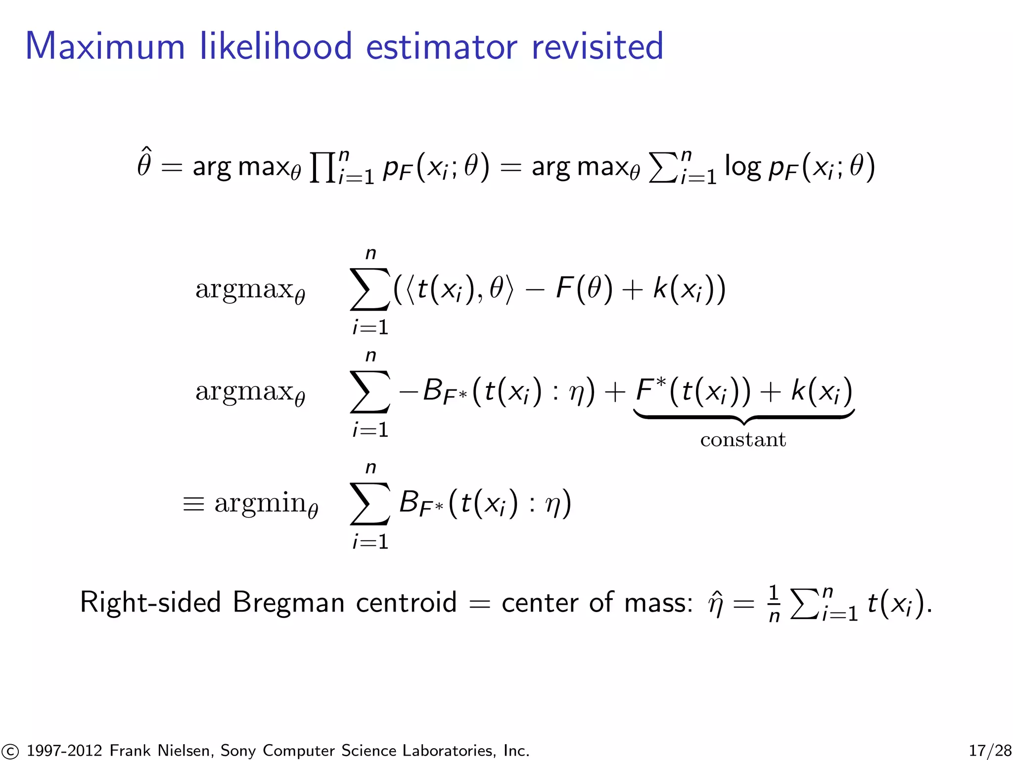
![Maximum Likelihood Estimator (MLE)
Given n identical and independently distributed observations
X = {x1, ..., xn}
Maximum Likelihood Estimator
Yn
ˆ= argmax2
i=1
pF (xi ; ) = argmax2ePn
i=1ht(xi ),i−F()+k(xi )
is unique maximum since r2F 0 (Hessian):
rF(ˆ) =
1
n
Xn
i=1
t(xi )
MLE is consistent, efficient with asymptotic normal distribution
ˆ N
,
1
n
I−1()
Fisher information matrix
I () = var[t(X)] = r2F()
MLE may be biased (eg, normal distributions).
c 1997-2012 Frank Nielsen, Sony Computer Science Laboratories, Inc. 14/28](https://image.slidesharecdn.com/kmle-talk-icassp2012-140902021340-phpapp02/75/k-MLE-A-fast-algorithm-for-learning-statistical-mixture-models-14-2048.jpg)
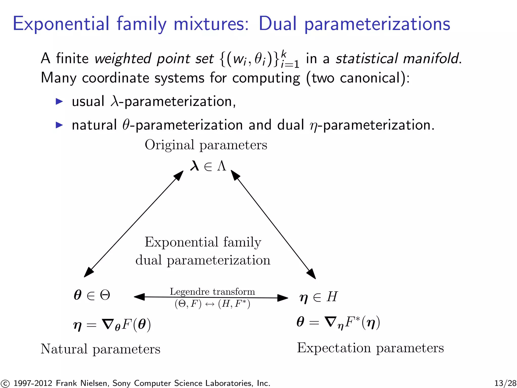
![Duality Bregman $ Exponential families [2]
Bregman divergence:
BF (x : )
Bregman generator:
F()
Cumulant function:
F()
Exponential family:
pF (x|)
Legendre
duality
= rF()
An exponential family...
pF (x; ) = exp(ht(x), i − F() + k(x))
has the log-density interpreted as a Bregman divergence:
log pF (x; ) = −BF(t(x) : ) + F(t(x)) + k(x)
c 1997-2012 Frank Nielsen, Sony Computer Science Laboratories, Inc. 15/28](https://image.slidesharecdn.com/kmle-talk-icassp2012-140902021340-phpapp02/75/k-MLE-A-fast-algorithm-for-learning-statistical-mixture-models-15-2048.jpg)
![Exponential families , Bregman divergences: Examples
F(x) pF (x|) , BF
Generator Exponential Family , Dual Bregman divergence
x2 Spherical Gaussian , Squared loss
x log x Multinomial , Kullback-Leibler divergence
x log x − x Poisson , I -divergence
−log(−2x) Rayleigh , Itakura-Saito divergence
−log x Geometric , Itakura-Saito divergence
log |X| Wishart , log-det/Burg matrix div. [8]
c 1997-2012 Frank Nielsen, Sony Computer Science Laboratories, Inc. 16/28](https://image.slidesharecdn.com/kmle-talk-icassp2012-140902021340-phpapp02/75/k-MLE-A-fast-algorithm-for-learning-statistical-mixture-models-16-2048.jpg)
![Bregman batched Lloyd’s k-means [2]
Extends Lloyd’s k-means heuristic to Bregman divergences.
I Initialize distinct seeds: C1 = P1, ..., Ck = Pk
I Repeat until convergence
I Assign point Pi to its “closest” centroid (wrt. BF (Pi : C))
Ci = {P 2 P | BF (P : Ci ) BF (P : Cj ) 8j6= i}
I Update cluster centroids by taking their center of mass:
Ci = 1
|Ci |
P
P2Ci
P.
Loss function
LF (P : C) =
X
P2P
BF (P : C)
BF (P : C) = min
i2{1,...,k}
BF (P : Ci )
...monotonically decreases and converges to a local optimum.
(Extend to weighted point sets using barycenters.)
c 1997-2012 Frank Nielsen, Sony Computer Science Laboratories, Inc. 18/28](https://image.slidesharecdn.com/kmle-talk-icassp2012-140902021340-phpapp02/75/k-MLE-A-fast-algorithm-for-learning-statistical-mixture-models-18-2048.jpg)
![k-MLE for EFMM Bregman Hard Clustering [4]
Bijection exponential families (distributions) $ Bregman distances
log pF (x; ) = −BF(t(x) : ) + F(t(x)) + k(x), = rF()
Bregman k-MLE for EFMMs (F) = additively weighted Bregman
hard k-means for F in the Qspace {yi = t(xi )}i :
Complete log-likelihood log
n
i=1
Qk
j=1(wjpF (xi |j ))j (zi ):
= max
,w
Xn
i=1
Xk
j=1
j (zi )(log pF (xi |j ) + log wj )
min
H,w
Xn
i=1
Xk
j=1
j (zi )((BF (t(xi ) : j ) − log wj )−k(xi ) − F(t(xi ) | {z }
constant
)
min
,w
Xn
i=1
k
min
j=1
BF(t(xi ) : j ) − log wj
(This is the argmin that gives the zi ’s)
c 1997-2012 Frank Nielsen, Sony Computer Science Laboratories, Inc. 19/28](https://image.slidesharecdn.com/kmle-talk-icassp2012-140902021340-phpapp02/75/k-MLE-A-fast-algorithm-for-learning-statistical-mixture-models-19-2048.jpg)
![k-MLE-EFMM algorithm [4]
I 0. Initialization: 8i 2 {1, ..., k}, let wi = 1
k and i = t(xi )
(initialization is further discussed later on).
I 1. Assignment:
8i 2 {1, ..., n}, zi = argminkj
=1BF(t(xi ) : j ) − log wj .
Let Ci = {xj |zj = i}, 8i 2 {1, ..., k} be the cluster partition:
X = [ki
=1Ci .
I 2. Update the -parameters:
P
8i 2 {1, ..., k}, 1
i = |Ci |
x2Ci
t(x).
Goto step 1 unless local convergence of the complete
likelihood is reached.
I 3. Update the mixture weights: 8i 2 {1, ..., k},wi = 1
n |Ci |.
Goto step 1 unless local convergence of the complete
likelihood is reached.
c 1997-2012 Frank Nielsen, Sony Computer Science Laboratories, Inc. 21/28](https://image.slidesharecdn.com/kmle-talk-icassp2012-140902021340-phpapp02/75/k-MLE-A-fast-algorithm-for-learning-statistical-mixture-models-21-2048.jpg)
![k-MLE initialization
I Forgy’s random seed (d = D),
I Bregman k-means (for F on Y, and MLE on each cluster).
Usually D d (eg., multivariate Gaussians D = d(d+3)
2 )
I Compute global MLE ˆ = 1
n
Pn
i=1 t(xi )
(well-defined for n D ! ˆ 2 )
I Consider restricted exponential family for Fˆ(d+1...D)((1...d)),
i = t(1...d)(xi ) and (d+1...D)
then set (1...d)
i = ˆ(d+1...D).
(e.g., we fix global covariance matrix, and let μi = xi for
Gaussians)
I Improve initialization by applying Bregman k-means++ [1] for
the convex conjugate of Fˆ(d+1...D)((1...d))
k-MLE++ based on Bregman k-means++
c 1997-2012 Frank Nielsen, Sony Computer Science Laboratories, Inc. 22/28](https://image.slidesharecdn.com/kmle-talk-icassp2012-140902021340-phpapp02/75/k-MLE-A-fast-algorithm-for-learning-statistical-mixture-models-22-2048.jpg)

![Expectation-maximization (EM) for EFMMs [2]
EM increases monotonically the expected complete likelihood
(marginalize):
Xn
i=1
Xk
j=1
p(zj |xi , ) log p(xi , zj |)
Banerjee et al. [2] proved it amounts to a Bregman soft clustering:
c 1997-2012 Frank Nielsen, Sony Computer Science Laboratories, Inc. 27/28](https://image.slidesharecdn.com/kmle-talk-icassp2012-140902021340-phpapp02/75/k-MLE-A-fast-algorithm-for-learning-statistical-mixture-models-30-2048.jpg)
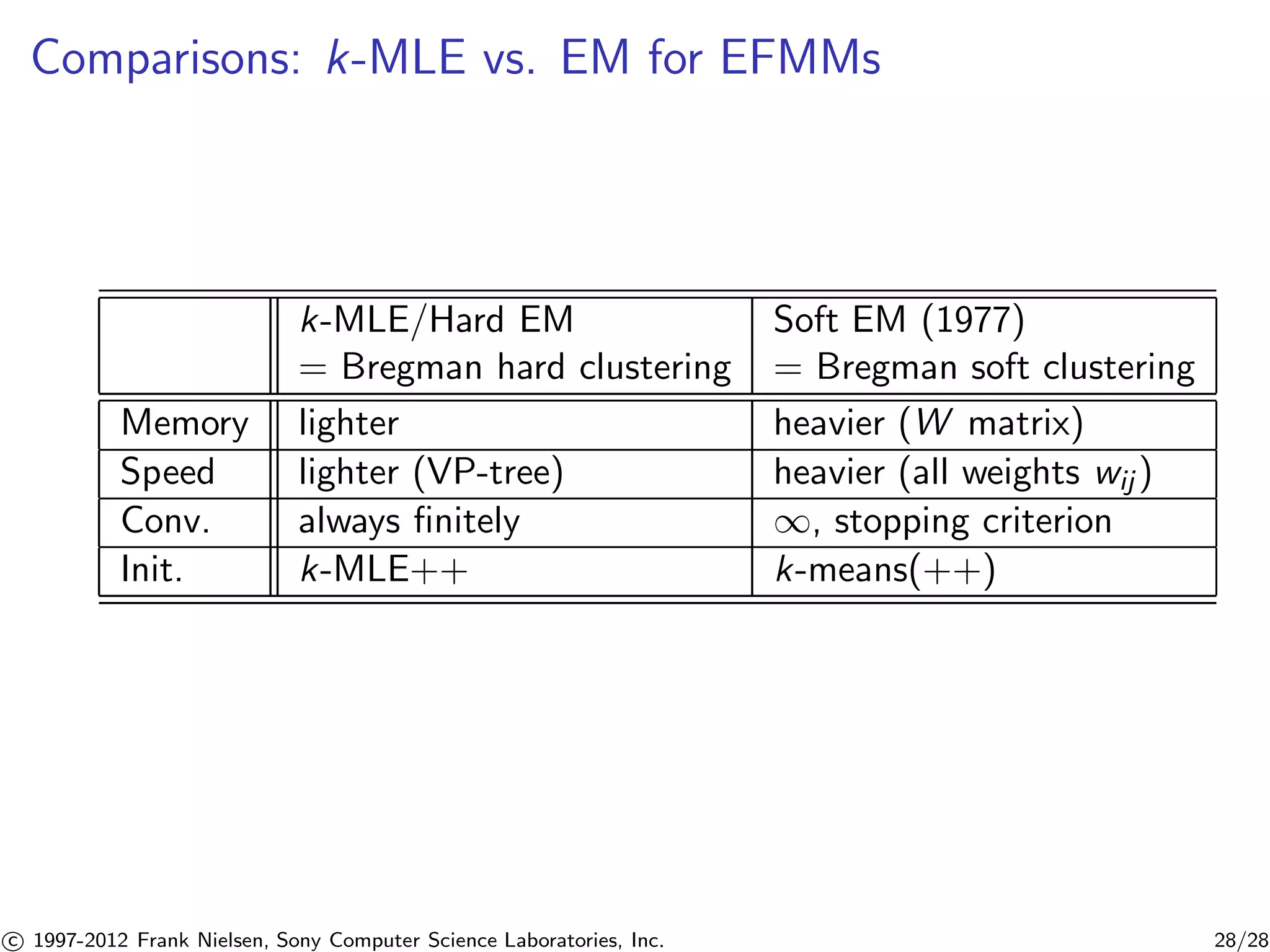

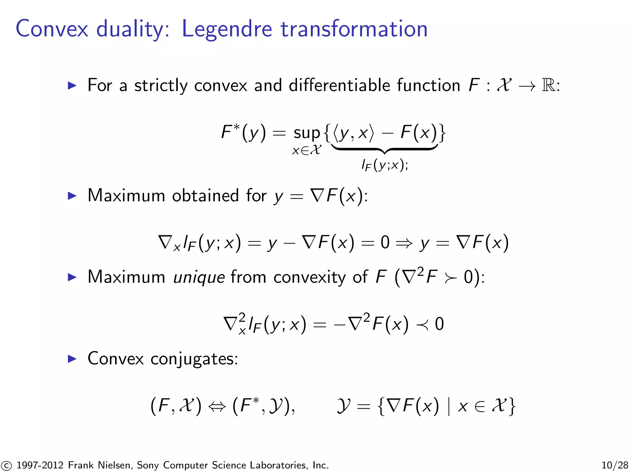
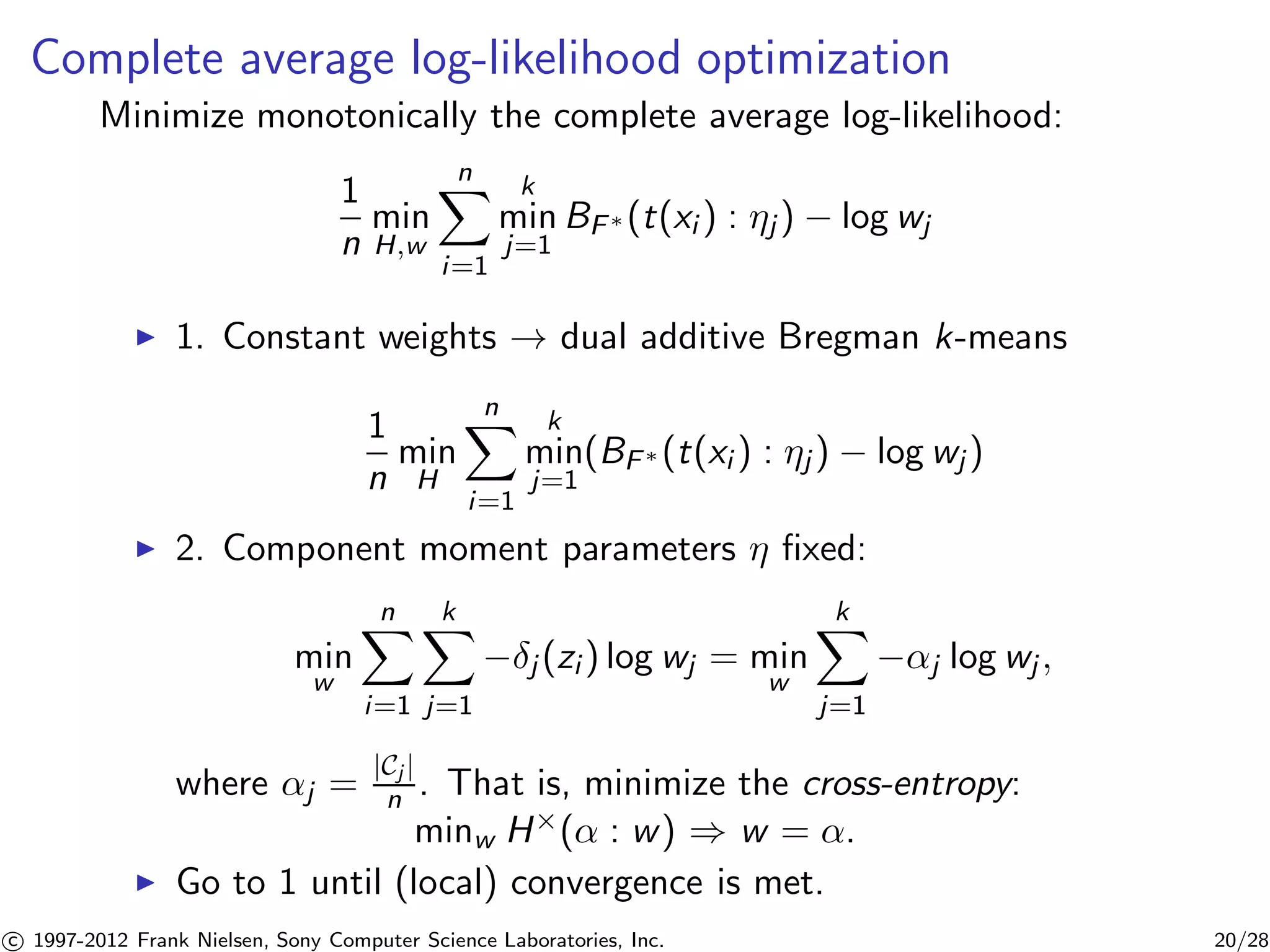
This document describes a fast algorithm called k-MLE for learning statistical mixture models. k-MLE is based on the connection between exponential family mixture models and Bregman divergences. It extends Lloyd's k-means clustering algorithm to optimize the complete log-likelihood of an exponential family mixture model using Bregman divergences. The algorithm iterates between assigning data points to clusters based on Bregman divergence, and updating the cluster parameters by taking the Bregman centroid of each cluster's assigned points. This provides a fast method for maximum likelihood estimation of exponential family mixture models.