Download as PDF, PPTX

![MCMC and Likelihood-free Methods
Computational issues in Bayesian statistics
Latent variables
Simple mixture (2)
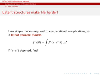
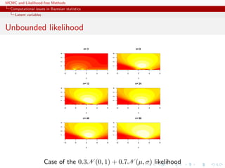
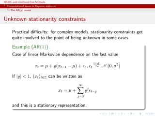
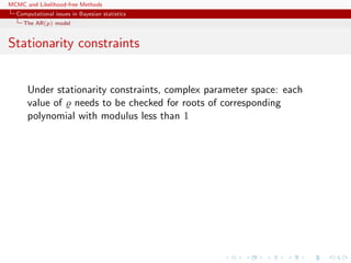
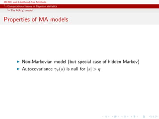
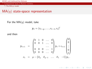
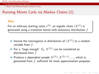
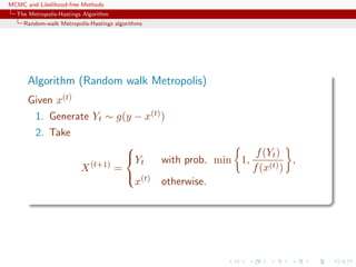
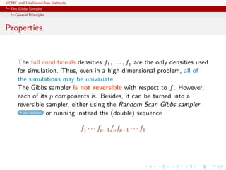
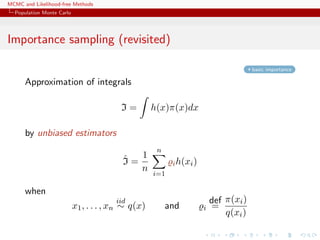
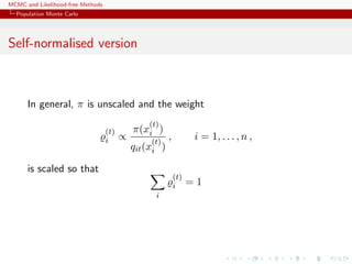
For the mixture of two normal distributions,
0.3N(µ1, 1) + 0.7N(µ2, 1) ,
likelihood proportional to
n
i=1
[0.3ϕ (xi − µ1) + 0.7 ϕ (xi − µ2)]
containing 2n terms.](https://image.slidesharecdn.com/abc-101023112352-phpapp01/85/MCMC-and-likelihood-free-methods-11-320.jpg)
![MCMC and Likelihood-free Methods
Computational issues in Bayesian statistics
Latent variables
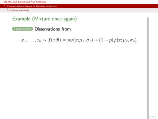
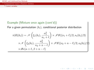
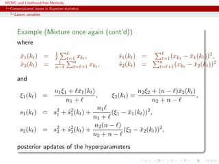
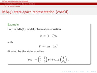
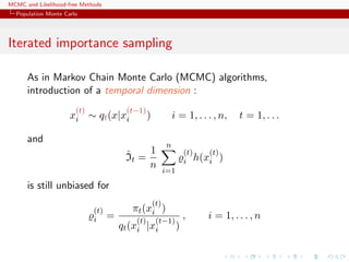
Example (Mixture once again)
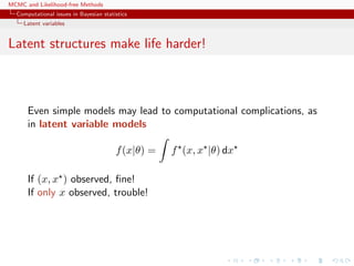
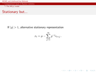
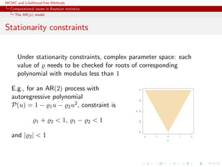
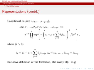
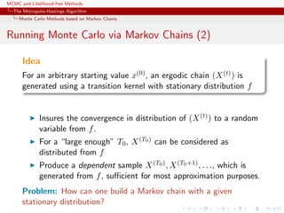
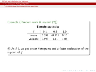
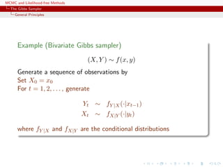
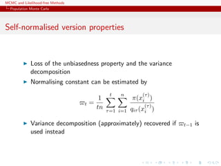
Bayes estimator of θ:
δπ
(x1, . . . , xn) =
n
=0 (kt)
ω(kt)Eπ
[θ|x, (kt)]
Too costly: 2n terms](https://image.slidesharecdn.com/abc-101023112352-phpapp01/85/MCMC-and-likelihood-free-methods-20-320.jpg)
![MCMC and Likelihood-free Methods
Computational issues in Bayesian statistics
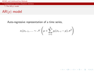
The MA(q) model
Representations
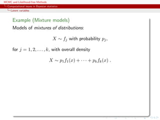
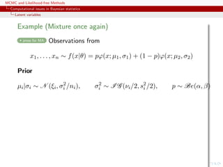
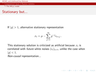
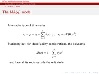
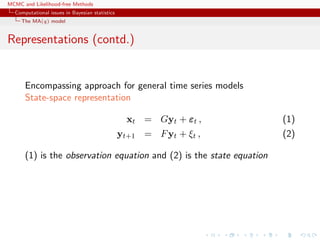
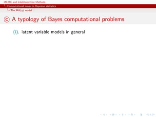
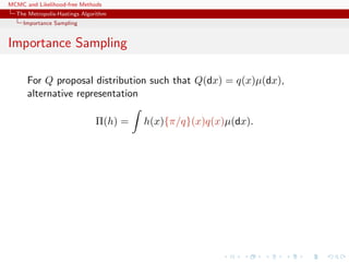
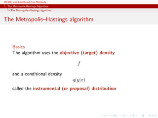
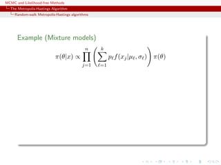
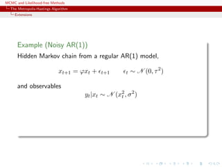
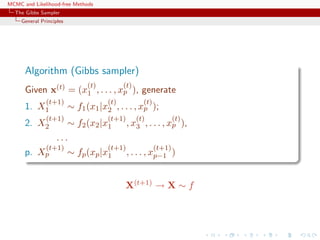
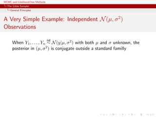
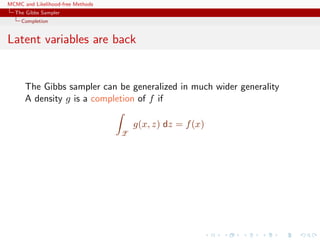
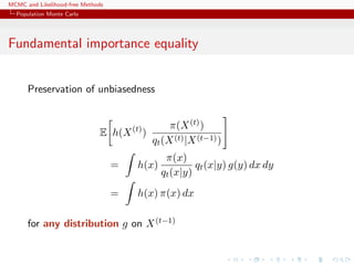
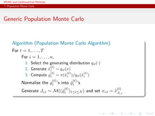
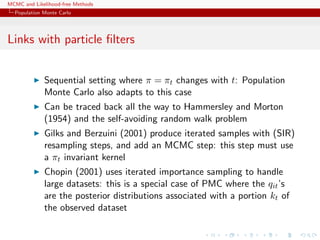
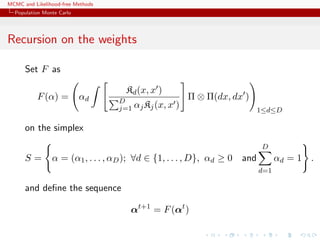
x1:T is a normal random variable with constant mean µ and
covariance matrix
Σ =
σ2
γ1 γ2 . . . γq 0 . . . 0 0
γ1 σ2
γ1 . . . γq−1 γq . . . 0 0
...
0 0 0 . . . 0 0 . . . γ1 σ2
,
with (|s| ≤ q)
γs = σ2
q−|s|
i=0
ϑiϑi+|s|
Not manageable in practice [large T’s]](https://image.slidesharecdn.com/abc-101023112352-phpapp01/85/MCMC-and-likelihood-free-methods-32-320.jpg)
![MCMC and Likelihood-free Methods
The Metropolis-Hastings Algorithm
Monte Carlo basics
Monte Carlo 101
Generate an iid sample x1, . . . , xN from π and estimate Π(h) by
ˆΠMC
N (h) = N−1
N
i=1
h(xi).
LLN: ˆΠMC
N (h)
as
−→ Π(h)
If Π(h2) = h2(x)π(x)µ(dx) < ∞,
CLT:
√
N ˆΠMC
N (h) − Π(h)
L
N 0, Π [h − Π(h)]2
.](https://image.slidesharecdn.com/abc-101023112352-phpapp01/85/MCMC-and-likelihood-free-methods-46-320.jpg)
![MCMC and Likelihood-free Methods
The Metropolis-Hastings Algorithm
Monte Carlo basics
Monte Carlo 101
Generate an iid sample x1, . . . , xN from π and estimate Π(h) by
ˆΠMC
N (h) = N−1
N
i=1
h(xi).
LLN: ˆΠMC
N (h)
as
−→ Π(h)
If Π(h2) = h2(x)π(x)µ(dx) < ∞,
CLT:
√
N ˆΠMC
N (h) − Π(h)
L
N 0, Π [h − Π(h)]2
.
Caveat announcing MCMC
Often impossible or inefficient to simulate directly from Π](https://image.slidesharecdn.com/abc-101023112352-phpapp01/85/MCMC-and-likelihood-free-methods-47-320.jpg)
![MCMC and Likelihood-free Methods
The Metropolis-Hastings Algorithm
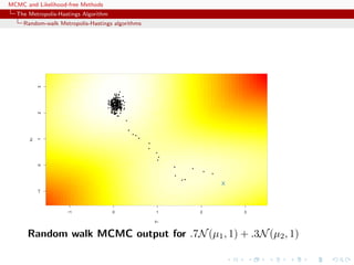
Random-walk Metropolis-Hastings algorithms
Example (Random walk and normal target)
forget History! Generate N(0, 1) based on the uniform proposal [−δ, δ]
[Hastings (1970)]
The probability of acceptance is then
ρ(x(t)
, yt) = exp{(x(t)2
− y2
t )/2} ∧ 1.](https://image.slidesharecdn.com/abc-101023112352-phpapp01/85/MCMC-and-likelihood-free-methods-71-320.jpg)
![MCMC and Likelihood-free Methods
The Metropolis-Hastings Algorithm
Random-walk Metropolis-Hastings algorithms
-1 0 1 2
050100150200250
(a)
-1.5-1.0-0.50.00.5
-2 0 2
0100200300400
(b) -1.5-1.0-0.50.00.5
-3 -2 -1 0 1 2 3
0100200300400
(c)
-1.5-1.0-0.50.00.5
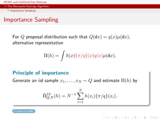
Three samples based on U[−δ, δ] with (a) δ = 0.1, (b) δ = 0.5
and (c) δ = 1.0, superimposed with the convergence of the
means (15, 000 simulations).](https://image.slidesharecdn.com/abc-101023112352-phpapp01/85/MCMC-and-likelihood-free-methods-73-320.jpg)
![MCMC and Likelihood-free Methods
The Metropolis-Hastings Algorithm
Random-walk Metropolis-Hastings algorithms
p
theta
0.0 0.2 0.4 0.6 0.8 1.0
-1012
tau
theta
0.2 0.4 0.6 0.8 1.0 1.2
-1012
p
tau
0.0 0.2 0.4 0.6 0.8 1.0
0.20.40.60.81.01.2
-1 0 1 2
0.01.02.0
theta
0.2 0.4 0.6 0.8
024
tau
0.0 0.2 0.4 0.6 0.8 1.0
0123456
p
Random walk sampling (50000 iterations)
General case of a 3 component normal mixture
[Celeux & al., 2000]](https://image.slidesharecdn.com/abc-101023112352-phpapp01/85/MCMC-and-likelihood-free-methods-76-320.jpg)
![MCMC and Likelihood-free Methods
The Metropolis-Hastings Algorithm
Random-walk Metropolis-Hastings algorithms
Convergence properties
Uniform ergodicity prohibited by random walk structure
At best, geometric ergodicity:
Theorem (Sufficient ergodicity)
For a symmetric density f, log-concave in the tails, and a positive
and symmetric density g, the chain (X(t)) is geometrically ergodic.
[Mengersen & Tweedie, 1996]
no tail effect](https://image.slidesharecdn.com/abc-101023112352-phpapp01/85/MCMC-and-likelihood-free-methods-79-320.jpg)
![MCMC and Likelihood-free Methods
The Metropolis-Hastings Algorithm
Random-walk Metropolis-Hastings algorithms
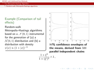
Further convergence properties
Under assumptions skip detailed convergence
(A1) f is super-exponential, i.e. it is positive with positive
continuous first derivative such that
lim|x|→∞ n(x) log f(x) = −∞ where n(x) := x/|x|.
In words : exponential decay of f in every direction with rate
tending to ∞
(A2) lim sup|x|→∞ n(x) m(x) < 0, where
m(x) = f(x)/| f(x)|.
In words: non degeneracy of the countour manifold
Cf(y) = {y : f(y) = f(x)}
Q is geometrically ergodic, and
V (x) ∝ f(x)−1/2 verifies the drift condition
[Jarner & Hansen, 2000]](https://image.slidesharecdn.com/abc-101023112352-phpapp01/85/MCMC-and-likelihood-free-methods-81-320.jpg)
![MCMC and Likelihood-free Methods
The Metropolis-Hastings Algorithm
Random-walk Metropolis-Hastings algorithms
Further [further] convergence properties
skip hyperdetailed convergence
If P ψ-irreducible and aperiodic, for r = (r(n))n∈N real-valued non
decreasing sequence, such that, for all n, m ∈ N,
r(n + m) ≤ r(n)r(m),
and r(0) = 1, for C a small set, τC = inf{n ≥ 1, Xn ∈ C}, and
h ≥ 1, assume
sup
x∈C
Ex
τC −1
k=0
r(k)h(Xk) < ∞,](https://image.slidesharecdn.com/abc-101023112352-phpapp01/85/MCMC-and-likelihood-free-methods-82-320.jpg)
![MCMC and Likelihood-free Methods
The Metropolis-Hastings Algorithm
Random-walk Metropolis-Hastings algorithms
then,
S(f, C, r) := x ∈ X, Ex
τC −1
k=0
r(k)h(Xk) < ∞
is full and absorbing and for x ∈ S(f, C, r),
lim
n→∞
r(n) Pn
(x, .) − f h = 0.
[Tuominen & Tweedie, 1994]](https://image.slidesharecdn.com/abc-101023112352-phpapp01/85/MCMC-and-likelihood-free-methods-83-320.jpg)
![MCMC and Likelihood-free Methods
The Metropolis-Hastings Algorithm
Random-walk Metropolis-Hastings algorithms
Comments
[CLT, Rosenthal’s inequality...] h-ergodicity implies CLT
for additive (possibly unbounded) functionals of the chain,
Rosenthal’s inequality and so on...
[Control of the moments of the return-time] The
condition implies (because h ≥ 1) that
sup
x∈C
Ex[r0(τC)] ≤ sup
x∈C
Ex
τC −1
k=0
r(k)h(Xk) < ∞,
where r0(n) = n
l=0 r(l) Can be used to derive bounds for
the coupling time, an essential step to determine computable
bounds, using coupling inequalities
[Roberts & Tweedie, 1998; Fort & Moulines, 2000]](https://image.slidesharecdn.com/abc-101023112352-phpapp01/85/MCMC-and-likelihood-free-methods-84-320.jpg)
![MCMC and Likelihood-free Methods
The Metropolis-Hastings Algorithm
Random-walk Metropolis-Hastings algorithms
Alternative conditions
The condition is not really easy to work with...
[Possible alternative conditions]
(a) [Tuominen, Tweedie, 1994] There exists a sequence
(Vn)n∈N, Vn ≥ r(n)h, such that
(i) supC V0 < ∞,
(ii) {V0 = ∞} ⊂ {V1 = ∞} and
(iii) PVn+1 ≤ Vn − r(n)h + br(n)IC.](https://image.slidesharecdn.com/abc-101023112352-phpapp01/85/MCMC-and-likelihood-free-methods-85-320.jpg)
![MCMC and Likelihood-free Methods
The Metropolis-Hastings Algorithm
Random-walk Metropolis-Hastings algorithms
(b) [Fort 2000] ∃V ≥ f ≥ 1 and b < ∞, such that supC V < ∞
and
PV (x) + Ex
σC
k=0
∆r(k)f(Xk) ≤ V (x) + bIC(x)
where σC is the hitting time on C and
∆r(k) = r(k) − r(k − 1), k ≥ 1 and ∆r(0) = r(0).
Result (a) ⇔ (b) ⇔ supx∈C Ex
τC −1
k=0 r(k)f(Xk) < ∞.](https://image.slidesharecdn.com/abc-101023112352-phpapp01/85/MCMC-and-likelihood-free-methods-86-320.jpg)
![MCMC and Likelihood-free Methods
The Metropolis-Hastings Algorithm
Extensions
MH correction
Accept the new value Yt with probability
f(Yt)
f(x(t))
·
exp − Yt − x(t) − σ2
2 log f(x(t))
2
2σ2
exp − x(t) − Yt − σ2
2 log f(Yt)
2
2σ2
∧ 1 .
Choice of the scaling factor σ
Should lead to an acceptance rate of 0.574 to achieve optimal
convergence rates (when the components of x are uncorrelated)
[Roberts & Rosenthal, 1998; Girolami & Calderhead, 2011]](https://image.slidesharecdn.com/abc-101023112352-phpapp01/85/MCMC-and-likelihood-free-methods-90-320.jpg)
![MCMC and Likelihood-free Methods
The Metropolis-Hastings Algorithm
Extensions
Rule of thumb
In small dimensions, aim at an average acceptance rate of 50%. In
large dimensions, at an average acceptance rate of 25%.
[Gelman,Gilks and Roberts, 1995]](https://image.slidesharecdn.com/abc-101023112352-phpapp01/85/MCMC-and-likelihood-free-methods-95-320.jpg)
![MCMC and Likelihood-free Methods
The Metropolis-Hastings Algorithm
Extensions
Rule of thumb
In small dimensions, aim at an average acceptance rate of 50%. In
large dimensions, at an average acceptance rate of 25%.
[Gelman,Gilks and Roberts, 1995]
This rule is to be taken with a pinch of salt!](https://image.slidesharecdn.com/abc-101023112352-phpapp01/85/MCMC-and-likelihood-free-methods-96-320.jpg)
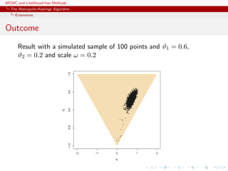
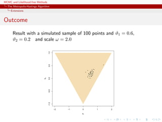
![MCMC and Likelihood-free Methods
The Metropolis-Hastings Algorithm
Extensions
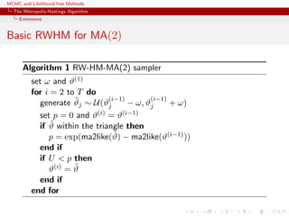
MA(2)
Since the constraints on (ϑ1, ϑ2) are well-defined, use of a flat
prior over the triangle as prior.
Simple representation of the likelihood
library(mnormt)
ma2like=function(theta){
n=length(y)
sigma = toeplitz(c(1 +theta[1]^2+theta[2]^2,
theta[1]+theta[1]*theta[2],theta[2],rep(0,n-3)))
dmnorm(y,rep(0,n),sigma,log=TRUE)
}](https://image.slidesharecdn.com/abc-101023112352-phpapp01/85/MCMC-and-likelihood-free-methods-102-320.jpg)


![MCMC and Likelihood-free Methods
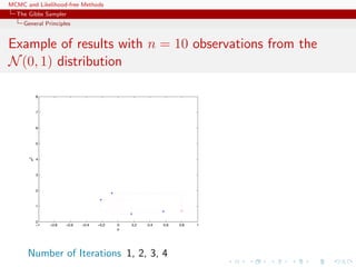
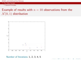
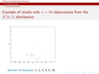
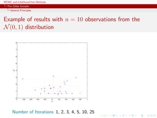
The Gibbs Sampler
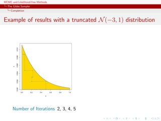
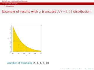
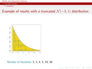
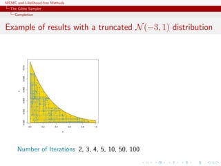
Completion
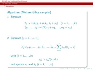
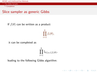
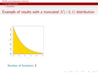
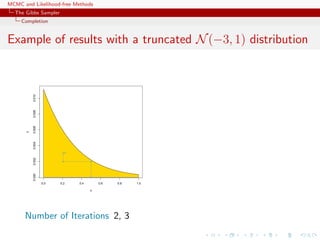
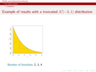
Algorithm (Slice sampler)
Simulate
1. ω
(t+1)
1 ∼ U[0,f1(θ(t))];
. . .
k. ω
(t+1)
k ∼ U[0,fk(θ(t))];
k+1. θ(t+1) ∼ UA(t+1) , with
A(t+1)
= {y; fi(y) ≥ ω
(t+1)
i , i = 1, . . . , k}.](https://image.slidesharecdn.com/abc-101023112352-phpapp01/85/MCMC-and-likelihood-free-methods-143-320.jpg)
![MCMC and Likelihood-free Methods
The Gibbs Sampler
Convergence
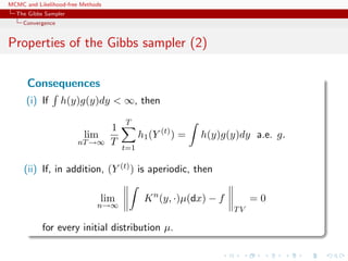
Properties of the Gibbs sampler
Theorem (Convergence)
For
(Y1, Y2, · · · , Yp) ∼ g(y1, . . . , yp),
if either
[Positivity condition]
(i) g(i)(yi) > 0 for every i = 1, · · · , p, implies that
g(y1, . . . , yp) > 0, where g(i) denotes the marginal distribution
of Yi, or
(ii) the transition kernel is absolutely continuous with respect to g,
then the chain is irreducible and positive Harris recurrent.](https://image.slidesharecdn.com/abc-101023112352-phpapp01/85/MCMC-and-likelihood-free-methods-155-320.jpg)
![MCMC and Likelihood-free Methods
The Gibbs Sampler
Convergence
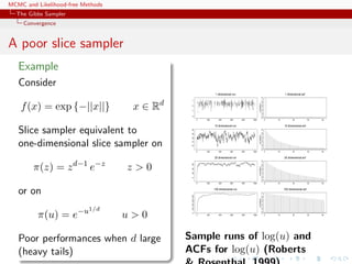
Slice sampler
fast on that slice
For convergence, the properties of Xt and of f(Xt) are identical
Theorem (Uniform ergodicity)
If f is bounded and suppf is bounded, the simple slice sampler is
uniformly ergodic.
[Mira & Tierney, 1997]](https://image.slidesharecdn.com/abc-101023112352-phpapp01/85/MCMC-and-likelihood-free-methods-157-320.jpg)
![MCMC and Likelihood-free Methods
The Gibbs Sampler
Convergence
A small set for a slice sampler
no slice detail
For > ,
C = {x ∈ X; < f(x) < }
is a small set:
Pr(x, ·) ≥ µ(·)
where
µ(A) =
1
0
λ(A ∩ L( ))
λ(L( ))
d
if L( ) = {x ∈ X; f(x) > }‘
[Roberts & Rosenthal, 1998]](https://image.slidesharecdn.com/abc-101023112352-phpapp01/85/MCMC-and-likelihood-free-methods-158-320.jpg)
![MCMC and Likelihood-free Methods
The Gibbs Sampler
Convergence
Slice sampler: drift
Under differentiability and monotonicity conditions, the slice
sampler also verifies a drift condition with V (x) = f(x)−β, is
geometrically ergodic, and there even exist explicit bounds on the
total variation distance
[Roberts & Rosenthal, 1998]](https://image.slidesharecdn.com/abc-101023112352-phpapp01/85/MCMC-and-likelihood-free-methods-159-320.jpg)
![MCMC and Likelihood-free Methods
The Gibbs Sampler
Convergence
Slice sampler: drift
Under differentiability and monotonicity conditions, the slice
sampler also verifies a drift condition with V (x) = f(x)−β, is
geometrically ergodic, and there even exist explicit bounds on the
total variation distance
[Roberts & Rosenthal, 1998]
Example (Exponential Exp(1))
For n > 23,
||Kn
(x, ·) − f(·)||TV ≤ .054865 (0.985015)n
(n − 15.7043)](https://image.slidesharecdn.com/abc-101023112352-phpapp01/85/MCMC-and-likelihood-free-methods-160-320.jpg)
![MCMC and Likelihood-free Methods
The Gibbs Sampler
Convergence
Slice sampler: convergence
no more slice detail
Theorem
For any density such that
∂
∂
λ ({x ∈ X; f(x) > }) is non-increasing
then
||K523
(x, ·) − f(·)||TV ≤ .0095
[Roberts & Rosenthal, 1998]](https://image.slidesharecdn.com/abc-101023112352-phpapp01/85/MCMC-and-likelihood-free-methods-161-320.jpg)
![MCMC and Likelihood-free Methods
The Gibbs Sampler
The Hammersley-Clifford theorem
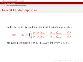
Hammersley-Clifford theorem
An illustration that conditionals determine the joint distribution
Theorem
If the joint density g(y1, y2) have conditional distributions
g1(y1|y2) and g2(y2|y1), then
g(y1, y2) =
g2(y2|y1)
g2(v|y1)/g1(y1|v) dv
.
[Hammersley & Clifford, circa 1970]](https://image.slidesharecdn.com/abc-101023112352-phpapp01/85/MCMC-and-likelihood-free-methods-163-320.jpg)
![MCMC and Likelihood-free Methods
Population Monte Carlo
Sequential variance decomposition
Furthermore,
var ˆIt =
1
n2
n
i=1
var
(t)
i h(x
(t)
i ) ,
if var
(t)
i exists, because the x
(t)
i ’s are conditionally uncorrelated
Note
This decomposition is still valid for correlated [in i] x
(t)
i ’s when
incorporating weights
(t)
i](https://image.slidesharecdn.com/abc-101023112352-phpapp01/85/MCMC-and-likelihood-free-methods-169-320.jpg)
![MCMC and Likelihood-free Methods
Population Monte Carlo
Special case of the product proposal
If
qt(x(t)
|x(t−1)
) =
n
i=1
qit(x
(t)
i |x(t−1)
)
[Independent proposals]
then
var ˆIt =
1
n2
n
i=1
var
(t)
i h(x
(t)
i ) ,](https://image.slidesharecdn.com/abc-101023112352-phpapp01/85/MCMC-and-likelihood-free-methods-171-320.jpg)
![MCMC and Likelihood-free Methods
Population Monte Carlo
Validation
skip validation
E
(t)
i h(X
(t)
i )
(t)
j h(X
(t)
j )
= h(xi)
π(xi)
qit(xi|x(t−1))
π(xj)
qjt(xj|x(t−1))
h(xj)
qit(xi|x(t−1)
) qjt(xj|x(t−1)
) dxi dxj g(x(t−1)
)dx(t−1)
= Eπ [h(X)]2
whatever the distribution g on x(t−1)](https://image.slidesharecdn.com/abc-101023112352-phpapp01/85/MCMC-and-likelihood-free-methods-172-320.jpg)
![MCMC and Likelihood-free Methods
Population Monte Carlo
Sampling importance resampling
Importance sampling from g can also produce samples from the
target π
[Rubin, 1987]](https://image.slidesharecdn.com/abc-101023112352-phpapp01/85/MCMC-and-likelihood-free-methods-175-320.jpg)
![MCMC and Likelihood-free Methods
Population Monte Carlo
Sampling importance resampling
Importance sampling from g can also produce samples from the
target π
[Rubin, 1987]
Theorem (Bootstraped importance sampling)
If a sample (xi )1≤i≤m is derived from the weighted sample
(xi, i)1≤i≤n by multinomial sampling with weights i, then
xi ∼ π(x)](https://image.slidesharecdn.com/abc-101023112352-phpapp01/85/MCMC-and-likelihood-free-methods-176-320.jpg)
![MCMC and Likelihood-free Methods
Population Monte Carlo
Sampling importance resampling
Importance sampling from g can also produce samples from the
target π
[Rubin, 1987]
Theorem (Bootstraped importance sampling)
If a sample (xi )1≤i≤m is derived from the weighted sample
(xi, i)1≤i≤n by multinomial sampling with weights i, then
xi ∼ π(x)
Note
Obviously, the xi ’s are not iid](https://image.slidesharecdn.com/abc-101023112352-phpapp01/85/MCMC-and-likelihood-free-methods-177-320.jpg)
![MCMC and Likelihood-free Methods
Population Monte Carlo
Iterated sampling importance resampling
This principle can be extended to iterated importance sampling:
After each iteration, resampling produces a sample from π
[Again, not iid!]](https://image.slidesharecdn.com/abc-101023112352-phpapp01/85/MCMC-and-likelihood-free-methods-178-320.jpg)
![MCMC and Likelihood-free Methods
Population Monte Carlo
Iterated sampling importance resampling
This principle can be extended to iterated importance sampling:
After each iteration, resampling produces a sample from π
[Again, not iid!]
Incentive
Use previous sample(s) to learn about π and q](https://image.slidesharecdn.com/abc-101023112352-phpapp01/85/MCMC-and-likelihood-free-methods-179-320.jpg)
![MCMC and Likelihood-free Methods
Population Monte Carlo
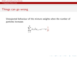
Illustration
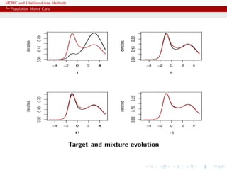
Example (A toy example)
Take the target
1/4N (−1, 0.3)(x) + 1/4N (0, 1)(x) + 1/2N (3, 2)(x)
and use 3 proposals: N (−1, 0.3), N (0, 1) and N (3, 2)
[Surprise!!!]](https://image.slidesharecdn.com/abc-101023112352-phpapp01/85/MCMC-and-likelihood-free-methods-197-320.jpg)
![MCMC and Likelihood-free Methods
Population Monte Carlo
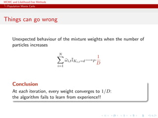
Illustration
Example (A toy example)
Take the target
1/4N (−1, 0.3)(x) + 1/4N (0, 1)(x) + 1/2N (3, 2)(x)
and use 3 proposals: N (−1, 0.3), N (0, 1) and N (3, 2)
[Surprise!!!]
Then
1 0.0500000 0.05000000 0.9000000
2 0.2605712 0.09970292 0.6397259
6 0.2740816 0.19160178 0.5343166
10 0.2989651 0.19200904 0.5090259
16 0.2651511 0.24129039 0.4935585
Weight evolution](https://image.slidesharecdn.com/abc-101023112352-phpapp01/85/MCMC-and-likelihood-free-methods-198-320.jpg)
![MCMC and Likelihood-free Methods
Population Monte Carlo
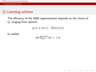
c Learning scheme
The efficiency of the SNIS approximation depends on the choice of
Q, ranging from optimal
q(x) ∝ |h(x) − Π(h)|π(x)
to useless
var ˆΠSNIS
Q,N (h) = +∞
Example (PMC=adaptive importance sampling)
Population Monte Carlo is producing a sequence of proposals Qt
aiming at improving efficiency
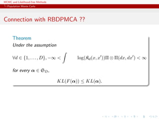
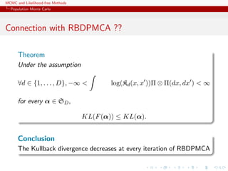
Kull(π, qt) ≤ Kull(π, qt−1) or var ˆΠSNIS
Qt,∞ (h) ≤ var ˆΠSNIS
Qt−1,∞(h)
[Capp´e, Douc, Guillin, Marin, Robert, 04, 07a, 07b, 08]](https://image.slidesharecdn.com/abc-101023112352-phpapp01/85/MCMC-and-likelihood-free-methods-201-320.jpg)
![MCMC and Likelihood-free Methods
Approximate Bayesian computation
ABC basics
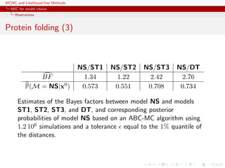
Illustrations
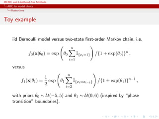
Example
Inference on CMB: in cosmology, study of the Cosmic Microwave
Background via likelihoods immensely slow to computate (e.g
WMAP, Plank), because of numerically costly spectral transforms
[Data is a Fortran program]
[Kilbinger et al., 2010, MNRAS]](https://image.slidesharecdn.com/abc-101023112352-phpapp01/85/MCMC-and-likelihood-free-methods-206-320.jpg)
![MCMC and Likelihood-free Methods
Approximate Bayesian computation
ABC basics
Illustrations
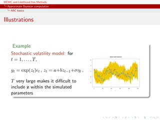
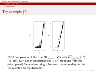
Example
Phylogenetic tree: in population
genetics, reconstitution of a common
ancestor from a sample of genes via
a phylogenetic tree that is close to
impossible to integrate out
[100 processor days with 4
parameters]
[Cornuet et al., 2009, Bioinformatics]](https://image.slidesharecdn.com/abc-101023112352-phpapp01/85/MCMC-and-likelihood-free-methods-207-320.jpg)
![MCMC and Likelihood-free Methods
Approximate Bayesian computation
ABC basics
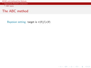
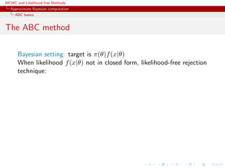
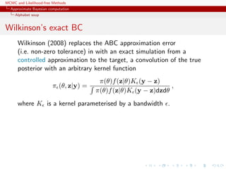
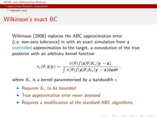
The ABC method
Bayesian setting: target is π(θ)f(x|θ)
When likelihood f(x|θ) not in closed form, likelihood-free rejection
technique:
ABC algorithm
For an observation y ∼ f(y|θ), under the prior π(θ), keep jointly
simulating
θ ∼ π(θ) , z ∼ f(z|θ ) ,
until the auxiliary variable z is equal to the observed value, z = y.
[Tavar´e et al., 1997]](https://image.slidesharecdn.com/abc-101023112352-phpapp01/85/MCMC-and-likelihood-free-methods-210-320.jpg)
![MCMC and Likelihood-free Methods
Approximate Bayesian computation
ABC basics
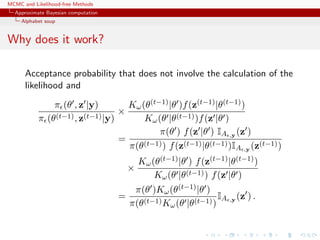
Why does it work?!
The proof is trivial:
f(θi) ∝
z∈D
π(θi)f(z|θi)Iy(z)
∝ π(θi)f(y|θi)
= π(θi|y) .
[Accept–Reject 101]](https://image.slidesharecdn.com/abc-101023112352-phpapp01/85/MCMC-and-likelihood-free-methods-211-320.jpg)
![MCMC and Likelihood-free Methods
Approximate Bayesian computation
ABC basics
Earlier occurrence
‘Bayesian statistics and Monte Carlo methods are ideally
suited to the task of passing many models over one
dataset’
[Don Rubin, Annals of Statistics, 1984]
Note Rubin (1984) does not promote this algorithm for
likelihood-free simulation but frequentist intuition on posterior
distributions: parameters from posteriors are more likely to be
those that could have generated the data.](https://image.slidesharecdn.com/abc-101023112352-phpapp01/85/MCMC-and-likelihood-free-methods-212-320.jpg)
![MCMC and Likelihood-free Methods
Approximate Bayesian computation
ABC basics
MA example
Back to the MA(q) model
xt = t +
q
i=1
ϑi t−i
Simple prior: uniform over the inverse [real and complex] roots in
Q(u) = 1 −
q
i=1
ϑiui
under the identifiability conditions](https://image.slidesharecdn.com/abc-101023112352-phpapp01/85/MCMC-and-likelihood-free-methods-218-320.jpg)
![MCMC and Likelihood-free Methods
Approximate Bayesian computation
ABC basics
Homonomy
The ABC algorithm is not to be confused with the ABC algorithm
The Artificial Bee Colony algorithm is a swarm based meta-heuristic
algorithm that was introduced by Karaboga in 2005 for optimizing
numerical problems. It was inspired by the intelligent foraging
behavior of honey bees. The algorithm is specifically based on the
model proposed by Tereshko and Loengarov (2005) for the foraging
behaviour of honey bee colonies. The model consists of three
essential components: employed and unemployed foraging bees, and
food sources. The first two components, employed and unemployed
foraging bees, search for rich food sources (...) close to their hive.
The model also defines two leading modes of behaviour (...):
recruitment of foragers to rich food sources resulting in positive
feedback and abandonment of poor sources by foragers causing
negative feedback.
[Karaboga, Scholarpedia]](https://image.slidesharecdn.com/abc-101023112352-phpapp01/85/MCMC-and-likelihood-free-methods-225-320.jpg)
![MCMC and Likelihood-free Methods
Approximate Bayesian computation
ABC basics
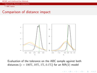
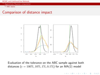
ABC advances
Simulating from the prior is often poor in efficiency
Either modify the proposal distribution on θ to increase the density
of x’s within the vicinity of y...
[Marjoram et al, 2003; Bortot et al., 2007, Sisson et al., 2007]](https://image.slidesharecdn.com/abc-101023112352-phpapp01/85/MCMC-and-likelihood-free-methods-227-320.jpg)
![MCMC and Likelihood-free Methods
Approximate Bayesian computation
ABC basics
ABC advances
Simulating from the prior is often poor in efficiency
Either modify the proposal distribution on θ to increase the density
of x’s within the vicinity of y...
[Marjoram et al, 2003; Bortot et al., 2007, Sisson et al., 2007]
...or by viewing the problem as a conditional density estimation
and by developing techniques to allow for larger
[Beaumont et al., 2002]](https://image.slidesharecdn.com/abc-101023112352-phpapp01/85/MCMC-and-likelihood-free-methods-228-320.jpg)
![MCMC and Likelihood-free Methods
Approximate Bayesian computation
ABC basics
ABC advances
Simulating from the prior is often poor in efficiency
Either modify the proposal distribution on θ to increase the density
of x’s within the vicinity of y...
[Marjoram et al, 2003; Bortot et al., 2007, Sisson et al., 2007]
...or by viewing the problem as a conditional density estimation
and by developing techniques to allow for larger
[Beaumont et al., 2002]
.....or even by including in the inferential framework [ABCµ]
[Ratmann et al., 2009]](https://image.slidesharecdn.com/abc-101023112352-phpapp01/85/MCMC-and-likelihood-free-methods-229-320.jpg)
![MCMC and Likelihood-free Methods
Approximate Bayesian computation
Alphabet soup
ABC-NP
Better usage of [prior] simulations by
adjustement: instead of throwing away
θ such that ρ(η(z), η(y)) > , replace
θs with locally regressed
θ∗
= θ − {η(z) − η(y)}T ˆβ
[Csill´ery et al., TEE, 2010]
where ˆβ is obtained by [NP] weighted least square regression on
(η(z) − η(y)) with weights
Kδ {ρ(η(z), η(y))}
[Beaumont et al., 2002, Genetics]](https://image.slidesharecdn.com/abc-101023112352-phpapp01/85/MCMC-and-likelihood-free-methods-230-320.jpg)
![MCMC and Likelihood-free Methods
Approximate Bayesian computation
Alphabet soup
ABC-MCMC
Markov chain (θ(t)) created via the transition function
θ(t+1)
=
θ ∼ Kω(θ |θ(t)) if x ∼ f(x|θ ) is such that x = y
and u ∼ U(0, 1) ≤ π(θ )Kω(θ(t)|θ )
π(θ(t))Kω(θ |θ(t))
,
θ(t) otherwise,
has the posterior π(θ|y) as stationary distribution
[Marjoram et al, 2003]](https://image.slidesharecdn.com/abc-101023112352-phpapp01/85/MCMC-and-likelihood-free-methods-232-320.jpg)
![MCMC and Likelihood-free Methods
Approximate Bayesian computation
Alphabet soup
ABC-MCMC (2)
Algorithm 3 Likelihood-free MCMC sampler
Use Algorithm 2 to get (θ(0), z(0))
for t = 1 to N do
Generate θ from Kω ·|θ(t−1) ,
Generate z from the likelihood f(·|θ ),
Generate u from U[0,1],
if u ≤ π(θ )Kω(θ(t−1)|θ )
π(θ(t−1)Kω(θ |θ(t−1))
IA ,y (z ) then
set (θ(t), z(t)) = (θ , z )
else
(θ(t), z(t))) = (θ(t−1), z(t−1)),
end if
end for](https://image.slidesharecdn.com/abc-101023112352-phpapp01/85/MCMC-and-likelihood-free-methods-233-320.jpg)
![MCMC and Likelihood-free Methods
Approximate Bayesian computation
Alphabet soup
ABCµ
[Ratmann, Andrieu, Wiuf and Richardson, 2009, PNAS]
Use of a joint density
f(θ, |y) ∝ ξ( |y, θ) × πθ(θ) × π ( )
where y is the data, and ξ( |y, θ) is the prior predictive density of
ρ(η(z), η(y)) given θ and x when z ∼ f(z|θ)](https://image.slidesharecdn.com/abc-101023112352-phpapp01/85/MCMC-and-likelihood-free-methods-235-320.jpg)
![MCMC and Likelihood-free Methods
Approximate Bayesian computation
Alphabet soup
ABCµ
[Ratmann, Andrieu, Wiuf and Richardson, 2009, PNAS]
Use of a joint density
f(θ, |y) ∝ ξ( |y, θ) × πθ(θ) × π ( )
where y is the data, and ξ( |y, θ) is the prior predictive density of
ρ(η(z), η(y)) given θ and x when z ∼ f(z|θ)
Warning! Replacement of ξ( |y, θ) with a non-parametric kernel
approximation.](https://image.slidesharecdn.com/abc-101023112352-phpapp01/85/MCMC-and-likelihood-free-methods-236-320.jpg)
![MCMC and Likelihood-free Methods
Approximate Bayesian computation
Alphabet soup
ABCµ details
Multidimensional distances ρk (k = 1, . . . , K) and errors
k = ρk(ηk(z), ηk(y)), with
k ∼ ξk( |y, θ) ≈ ˆξk( |y, θ) =
1
Bhk
b
K[{ k−ρk(ηk(zb), ηk(y))}/hk]
then used in replacing ξ( |y, θ) with mink
ˆξk( |y, θ)](https://image.slidesharecdn.com/abc-101023112352-phpapp01/85/MCMC-and-likelihood-free-methods-237-320.jpg)
![MCMC and Likelihood-free Methods
Approximate Bayesian computation
Alphabet soup
ABCµ details
Multidimensional distances ρk (k = 1, . . . , K) and errors
k = ρk(ηk(z), ηk(y)), with
k ∼ ξk( |y, θ) ≈ ˆξk( |y, θ) =
1
Bhk
b
K[{ k−ρk(ηk(zb), ηk(y))}/hk]
then used in replacing ξ( |y, θ) with mink
ˆξk( |y, θ)
ABCµ involves acceptance probability
π(θ , )
π(θ, )
q(θ , θ)q( , )
q(θ, θ )q( , )
mink
ˆξk( |y, θ )
mink
ˆξk( |y, θ)](https://image.slidesharecdn.com/abc-101023112352-phpapp01/85/MCMC-and-likelihood-free-methods-238-320.jpg)
![MCMC and Likelihood-free Methods
Approximate Bayesian computation
Alphabet soup
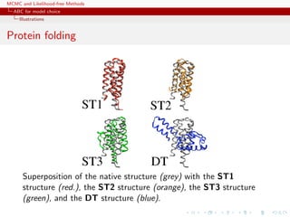
ABCµ multiple errors
[ c Ratmann et al., PNAS, 2009]](https://image.slidesharecdn.com/abc-101023112352-phpapp01/85/MCMC-and-likelihood-free-methods-239-320.jpg)
![MCMC and Likelihood-free Methods
Approximate Bayesian computation
Alphabet soup
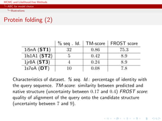
ABCµ for model choice
[ c Ratmann et al., PNAS, 2009]](https://image.slidesharecdn.com/abc-101023112352-phpapp01/85/MCMC-and-likelihood-free-methods-240-320.jpg)

![MCMC and Likelihood-free Methods
Approximate Bayesian computation
Alphabet soup
Questions about ABCµ
For each model under comparison, marginal posterior on used to
assess the fit of the model (HPD includes 0 or not).
Is the data informative about ? [Identifiability]
How is the prior π( ) impacting the comparison?
How is using both ξ( |x0, θ) and π ( ) compatible with a
standard probability model? [remindful of Wilkinson]
Where is the penalisation for complexity in the model
comparison?
[X, Mengersen & Chen, 2010, PNAS]](https://image.slidesharecdn.com/abc-101023112352-phpapp01/85/MCMC-and-likelihood-free-methods-242-320.jpg)
![MCMC and Likelihood-free Methods
Approximate Bayesian computation
Alphabet soup
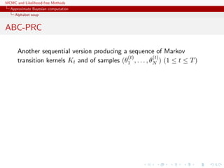
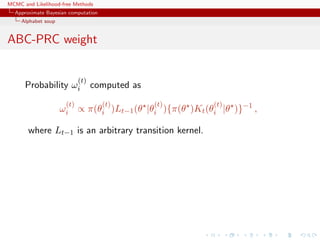
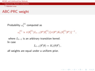
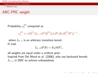
ABC-PRC
Another sequential version producing a sequence of Markov
transition kernels Kt and of samples (θ
(t)
1 , . . . , θ
(t)
N ) (1 ≤ t ≤ T)
ABC-PRC Algorithm
1. Pick a θ is selected at random among the previous θ
(t−1)
i ’s
with probabilities ω
(t−1)
i (1 ≤ i ≤ N).
2. Generate
θ
(t)
i ∼ Kt(θ|θ ) , x ∼ f(x|θ
(t)
i ) ,
3. Check that (x, y) < , otherwise start again.
[Sisson et al., 2007]](https://image.slidesharecdn.com/abc-101023112352-phpapp01/85/MCMC-and-likelihood-free-methods-244-320.jpg)
![MCMC and Likelihood-free Methods
Approximate Bayesian computation
Alphabet soup
Why PRC?
Partial rejection control: Resample from a population of weighted
particles by pruning away particles with weights below threshold C,
replacing them by new particles obtained by propagating an
existing particle by an SMC step and modifying the weights
accordinly.
[Liu, 2001]](https://image.slidesharecdn.com/abc-101023112352-phpapp01/85/MCMC-and-likelihood-free-methods-245-320.jpg)
![MCMC and Likelihood-free Methods
Approximate Bayesian computation
Alphabet soup
Why PRC?
Partial rejection control: Resample from a population of weighted
particles by pruning away particles with weights below threshold C,
replacing them by new particles obtained by propagating an
existing particle by an SMC step and modifying the weights
accordinly.
[Liu, 2001]
PRC justification in ABC-PRC:
Suppose we then implement the PRC algorithm for some
c > 0 such that only identically zero weights are smaller
than c
Trouble is, there is no such c...](https://image.slidesharecdn.com/abc-101023112352-phpapp01/85/MCMC-and-likelihood-free-methods-246-320.jpg)
![MCMC and Likelihood-free Methods
Approximate Bayesian computation
Alphabet soup
ABC-PRC bias
Lack of unbiasedness of the method
Joint density of the accepted pair (θ(t−1), θ(t)) proportional to
π(θ
(t−1)
|y)Kt(θ
(t)
|θ
(t−1)
)f(y|θ
(t)
) ,
For an arbitrary function h(θ), E[ωth(θ(t))] proportional to
ZZ
h(θ
(t)
)
π(θ(t)
)Lt−1(θ(t−1)
|θ(t)
)
π(θ(t−1))Kt(θ(t)|θ(t−1))
π(θ
(t−1)
|y)Kt(θ
(t)
|θ
(t−1)
)f(y|θ
(t)
)dθ
(t−1)
dθ
(t)
∝
ZZ
h(θ
(t)
)
π(θ(t)
)Lt−1(θ(t−1)
|θ(t)
)
π(θ(t−1))Kt(θ(t)|θ(t−1))
π(θ
(t−1)
)f(y|θ
(t−1)
)
× Kt(θ
(t)
|θ
(t−1)
)f(y|θ
(t)
)dθ
(t−1)
dθ
(t)
∝
Z
h(θ
(t)
)π(θ
(t)
|y)
Z
Lt−1(θ
(t−1)
|θ
(t)
)f(y|θ
(t−1)
)dθ
(t−1)
ff
dθ
(t)
.](https://image.slidesharecdn.com/abc-101023112352-phpapp01/85/MCMC-and-likelihood-free-methods-251-320.jpg)
![MCMC and Likelihood-free Methods
Approximate Bayesian computation
Alphabet soup
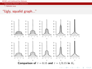
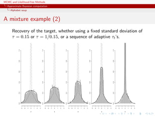
A mixture example (1)
Toy model of Sisson et al. (2007): if
θ ∼ U(−10, 10) , x|θ ∼ 0.5 N(θ, 1) + 0.5 N(θ, 1/100) ,
then the posterior distribution associated with y = 0 is the normal
mixture
θ|y = 0 ∼ 0.5 N(0, 1) + 0.5 N(0, 1/100)
restricted to [−10, 10].
Furthermore, true target available as
π(θ||x| < ) ∝ Φ( −θ)−Φ(− −θ)+Φ(10( −θ))−Φ(−10( +θ)) .](https://image.slidesharecdn.com/abc-101023112352-phpapp01/85/MCMC-and-likelihood-free-methods-252-320.jpg)
![MCMC and Likelihood-free Methods
Approximate Bayesian computation
Alphabet soup
A PMC version
Use of the same kernel idea as ABC-PRC but with IS correction
Generate a sample at iteration t by
ˆπt(θ(t)
) ∝
N
j=1
ω
(t−1)
j Kt(θ(t)
|θ
(t−1)
j )
modulo acceptance of the associated xt, and use an importance
weight associated with an accepted simulation θ
(t)
i
ω
(t)
i ∝ π(θ
(t)
i ) ˆπt(θ
(t)
i ) .
c Still likelihood free
[Beaumont et al., 2008, arXiv:0805.2256]](https://image.slidesharecdn.com/abc-101023112352-phpapp01/85/MCMC-and-likelihood-free-methods-254-320.jpg)
![MCMC and Likelihood-free Methods
Approximate Bayesian computation
Alphabet soup
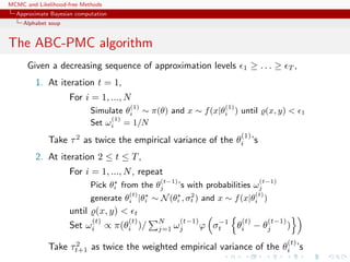
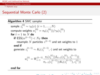
Sequential Monte Carlo
SMC is a simulation technique to approximate a sequence of
related probability distributions πn with π0 “easy” and πT as
target.
Iterated IS as PMC : particles moved from time n to time n via
kernel Kn and use of a sequence of extended targets ˜πn
˜πn(z0:n) = πn(zn)
n
j=0
Lj(zj+1, zj)
where the Lj’s are backward Markov kernels [check that πn(zn) is
a marginal]
[Del Moral, Doucet & Jasra, Series B, 2006]](https://image.slidesharecdn.com/abc-101023112352-phpapp01/85/MCMC-and-likelihood-free-methods-256-320.jpg)
![MCMC and Likelihood-free Methods
Approximate Bayesian computation
Alphabet soup
ABC-SMC
[Del Moral, Doucet & Jasra, 2009]
True derivation of an SMC-ABC algorithm
Use of a kernel Kn associated with target π n and derivation of the
backward kernel
Ln−1(z, z ) =
π n (z )Kn(z , z)
πn(z)
Update of the weights
win ∝ wi(n−1)
M
m=1 IA n
(xm
in)
M
m=1 IA n−1
(xm
i(n−1))
when xm
in ∼ K(xi(n−1), ·)](https://image.slidesharecdn.com/abc-101023112352-phpapp01/85/MCMC-and-likelihood-free-methods-258-320.jpg)
![MCMC and Likelihood-free Methods
Approximate Bayesian computation
Alphabet soup
ABC-SMCM
Modification: Makes M repeated simulations of the pseudo-data z
given the parameter, rather than using a single [M = 1]
simulation, leading to weight that is proportional to the number of
accepted zis
ω(θ) =
1
M
M
i=1
Iρ(η(y),η(zi))<
[limit in M means exact simulation from (tempered) target]](https://image.slidesharecdn.com/abc-101023112352-phpapp01/85/MCMC-and-likelihood-free-methods-259-320.jpg)
![MCMC and Likelihood-free Methods
Approximate Bayesian computation
Alphabet soup
Properties of ABC-SMC
The ABC-SMC method properly uses a backward kernel L(z, z ) to
simplify the importance weight and to remove the dependence on
the unknown likelihood from this weight. Update of importance
weights is reduced to the ratio of the proportions of surviving
particles
Major assumption: the forward kernel K is supposed to be
invariant against the true target [tempered version of the true
posterior]](https://image.slidesharecdn.com/abc-101023112352-phpapp01/85/MCMC-and-likelihood-free-methods-260-320.jpg)
![MCMC and Likelihood-free Methods
Approximate Bayesian computation
Alphabet soup
Properties of ABC-SMC
The ABC-SMC method properly uses a backward kernel L(z, z ) to
simplify the importance weight and to remove the dependence on
the unknown likelihood from this weight. Update of importance
weights is reduced to the ratio of the proportions of surviving
particles
Major assumption: the forward kernel K is supposed to be
invariant against the true target [tempered version of the true
posterior]
Adaptivity in ABC-SMC algorithm only found in on-line
construction of the thresholds t, slowly enough to keep a large
number of accepted transitions](https://image.slidesharecdn.com/abc-101023112352-phpapp01/85/MCMC-and-likelihood-free-methods-261-320.jpg)
![MCMC and Likelihood-free Methods
Approximate Bayesian computation
Alphabet soup
Semi-automatic ABC
Fearnhead and Prangle (2010) study ABC and the selection of the
summary statistic in close proximity to Wilkinson’s proposal
ABC then considered from a purely inferential viewpoint and
calibrated for estimation purposes.
Use of a randomised (or ‘noisy’) version of the summary statistics
˜η(y) = η(y) + τ
Derivation of a well-calibrated version of ABC, i.e. an algorithm
that gives proper predictions for the distribution associated with
this randomised summary statistic. [calibration constraint: ABC
approximation with same posterior mean as the true randomised
posterior.]](https://image.slidesharecdn.com/abc-101023112352-phpapp01/85/MCMC-and-likelihood-free-methods-266-320.jpg)
![MCMC and Likelihood-free Methods
Approximate Bayesian computation
Calibration of ABC
Which summary?
Fundamental difficulty of the choice of the summary statistic when
there is no non-trivial sufficient statistics [except when done by the
experimenters in the field]](https://image.slidesharecdn.com/abc-101023112352-phpapp01/85/MCMC-and-likelihood-free-methods-269-320.jpg)
![MCMC and Likelihood-free Methods
Approximate Bayesian computation
Calibration of ABC
Which summary?
Fundamental difficulty of the choice of the summary statistic when
there is no non-trivial sufficient statistics [except when done by the
experimenters in the field]
Starting from a large collection of summary statistics is available,
Joyce and Marjoram (2008) consider the sequential inclusion into
the ABC target, with a stopping rule based on a likelihood ratio
test.](https://image.slidesharecdn.com/abc-101023112352-phpapp01/85/MCMC-and-likelihood-free-methods-270-320.jpg)
![MCMC and Likelihood-free Methods
Approximate Bayesian computation
Calibration of ABC
Which summary?
Fundamental difficulty of the choice of the summary statistic when
there is no non-trivial sufficient statistics [except when done by the
experimenters in the field]
Starting from a large collection of summary statistics is available,
Joyce and Marjoram (2008) consider the sequential inclusion into
the ABC target, with a stopping rule based on a likelihood ratio
test.
Does not taking into account the sequential nature of the tests
Depends on parameterisation
Order of inclusion matters.](https://image.slidesharecdn.com/abc-101023112352-phpapp01/85/MCMC-and-likelihood-free-methods-271-320.jpg)
![MCMC and Likelihood-free Methods
Approximate Bayesian computation
Calibration of ABC
A connected Monte Carlo study
Repeating simulations of the pseudo-data per simulated parameter
does not improve approximation
Tolerance level does not seem to be highly influential
Choice of distance / summary statistics / calibration factors
are paramount to successful approximation
ABC-SMC outperforms ABC-MCMC
[Mckinley, Cook, Deardon, 2009]](https://image.slidesharecdn.com/abc-101023112352-phpapp01/85/MCMC-and-likelihood-free-methods-272-320.jpg)


![MCMC and Likelihood-free Methods
ABC for model choice
Model choice
ABC estimates
Posterior probability π(M = m|y) approximated by the frequency
of acceptances from model m
1
T
T
t=1
Im(t)=m .
Issues with implementation:
should tolerances be the same for all models?
should summary statistics vary across models (incl. their
dimension)?
should the distance measure ρ vary as well?
Extension to a weighted polychotomous logistic regression estimate
of π(M = m|y), with non-parametric kernel weights
[Cornuet et al., DIYABC, 2009]](https://image.slidesharecdn.com/abc-101023112352-phpapp01/85/MCMC-and-likelihood-free-methods-278-320.jpg)
![MCMC and Likelihood-free Methods
ABC for model choice
Model choice
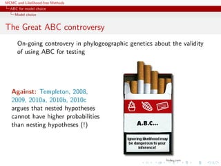
The Great ABC controversy
On-going controvery in phylogeographic genetics about the validity
of using ABC for testing
Against: Templeton, 2008,
2009, 2010a, 2010b, 2010c
argues that nested hypotheses
cannot have higher probabilities
than nesting hypotheses (!)
Replies: Fagundes et al., 2008,
Beaumont et al., 2010, Berger et
al., 2010, Csill`ery et al., 2010
point out that the criticisms are
addressed at [Bayesian]
model-based inference and have
nothing to do with ABC...](https://image.slidesharecdn.com/abc-101023112352-phpapp01/85/MCMC-and-likelihood-free-methods-280-320.jpg)
![MCMC and Likelihood-free Methods
ABC for model choice
Gibbs random fields
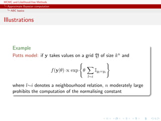
Potts model
Potts model
Vc(y) is of the form
Vc(y) = θS(y) = θ
l∼i
δyl=yi
where l∼i denotes a neighbourhood structure
In most realistic settings, summation
Zθ =
x∈X
exp{θT
S(x)}
involves too many terms to be manageable and numerical
approximations cannot always be trusted
[Cucala, Marin, CPR & Titterington, 2009]](https://image.slidesharecdn.com/abc-101023112352-phpapp01/85/MCMC-and-likelihood-free-methods-284-320.jpg)
![MCMC and Likelihood-free Methods
ABC for model choice
Model choice via ABC
Sufficient statistics
By definition, if S(x) sufficient statistic for the joint parameters
(M, θ0, . . . , θM−1),
P(M = m|x) = P(M = m|S(x)) .
For each model m, own sufficient statistic Sm(·) and
S(·) = (S0(·), . . . , SM−1(·)) also sufficient.
For Gibbs random fields,
x|M = m ∼ fm(x|θm) = f1
m(x|S(x))f2
m(S(x)|θm)
=
1
n(S(x))
f2
m(S(x)|θm)
where
n(S(x)) = {˜x ∈ X : S(˜x) = S(x)}
c S(x) is therefore also sufficient for the joint parameters
[Specific to Gibbs random fields!]](https://image.slidesharecdn.com/abc-101023112352-phpapp01/85/MCMC-and-likelihood-free-methods-292-320.jpg)

This document discusses computational issues that arise in Bayesian statistics. It provides examples of latent variable models like mixture models that make computation difficult due to the large number of terms that must be calculated. It also discusses time series models like the AR(p) and MA(q) models, noting that they have complex parameter spaces due to stationarity constraints. The document outlines the Metropolis-Hastings algorithm, Gibbs sampler, and other methods like Population Monte Carlo and Approximate Bayesian Computation that can help address these computational challenges.


![[A]BCel : a presentation at ABC in Roma](https://cdn.slidesharecdn.com/ss_thumbnails/abcel-130530042650-phpapp02-thumbnail.jpg?width=640&height=640&fit=bounds)


