Download as PDF, PPTX

![cantly
contribute to methodological developments of ABC.
[Grith al., 1997; Tavare al., 1999]](https://image.slidesharecdn.com/ho1wjotimgbqygqfye1g-signature-8be37557a25ca84b691076eb3d9b0b90d5f3cf9a8a52b597ab20c4e203a597cc-poli-141213034223-conversion-gate01/85/3rd-NIPS-Workshop-on-PROBABILISTIC-PROGRAMMING-18-320.jpg)
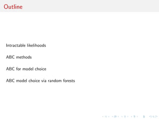
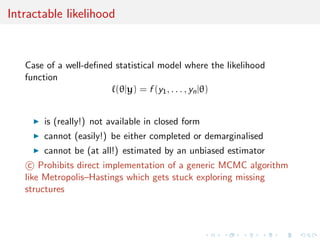
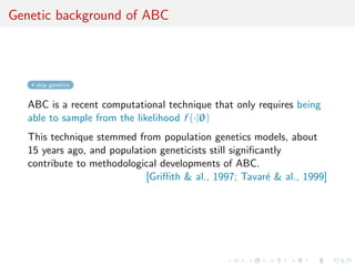
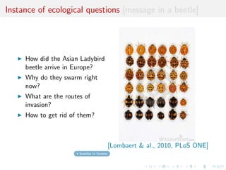
![Instance of ecological questions [message in a beetle]
I How did the Asian Ladybird
beetle arrive in Europe?
I Why do they swarm right
now?
I What are the routes of
invasion?
I How to get rid of them?
[Lombaert al., 2010, PLoS ONE]
beetles in forests](https://image.slidesharecdn.com/ho1wjotimgbqygqfye1g-signature-8be37557a25ca84b691076eb3d9b0b90d5f3cf9a8a52b597ab20c4e203a597cc-poli-141213034223-conversion-gate01/85/3rd-NIPS-Workshop-on-PROBABILISTIC-PROGRAMMING-24-320.jpg)
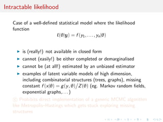
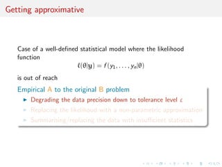
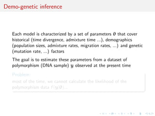
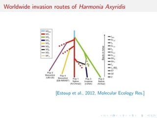
![Worldwide invasion routes of Harmonia Axyridis
[Estoup et al., 2012, Molecular Ecology Res.]](https://image.slidesharecdn.com/ho1wjotimgbqygqfye1g-signature-8be37557a25ca84b691076eb3d9b0b90d5f3cf9a8a52b597ab20c4e203a597cc-poli-141213034223-conversion-gate01/85/3rd-NIPS-Workshop-on-PROBABILISTIC-PROGRAMMING-25-320.jpg)
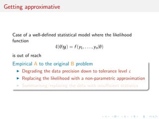
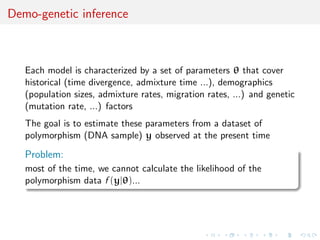
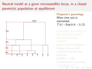
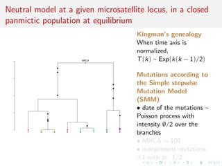
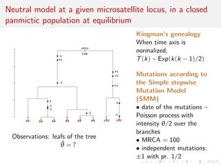
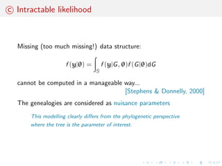
![c Intractable likelihood
Missing (too much missing!) data structure:
f (yj) =
Z
G
f (yjG, )f (Gj)dG
cannot be computed in a manageable way...
[Stephens Donnelly, 2000]
The genealogies are considered as nuisance parameters
This modelling clearly diers from the phylogenetic perspective
where the tree is the parameter of interest.](https://image.slidesharecdn.com/ho1wjotimgbqygqfye1g-signature-8be37557a25ca84b691076eb3d9b0b90d5f3cf9a8a52b597ab20c4e203a597cc-poli-141213034223-conversion-gate01/85/3rd-NIPS-Workshop-on-PROBABILISTIC-PROGRAMMING-26-320.jpg)
![c Intractable likelihood
Missing (too much missing!) data structure:
f (yj) =
Z
G
f (yjG, )f (Gj)dG
cannot be computed in a manageable way...
[Stephens Donnelly, 2000]
The genealogies are considered as nuisance parameters
This modelling clearly diers from the phylogenetic perspective
where the tree is the parameter of interest.](https://image.slidesharecdn.com/ho1wjotimgbqygqfye1g-signature-8be37557a25ca84b691076eb3d9b0b90d5f3cf9a8a52b597ab20c4e203a597cc-poli-141213034223-conversion-gate01/85/3rd-NIPS-Workshop-on-PROBABILISTIC-PROGRAMMING-27-320.jpg)
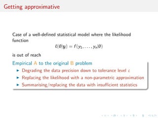
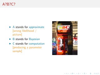
![A?B?C?
I A stands for approximate
[wrong likelihood /
picture]
I B stands for Bayesian
I C stands for computation
[producing a parameter
sample]](https://image.slidesharecdn.com/ho1wjotimgbqygqfye1g-signature-8be37557a25ca84b691076eb3d9b0b90d5f3cf9a8a52b597ab20c4e203a597cc-poli-141213034223-conversion-gate01/85/3rd-NIPS-Workshop-on-PROBABILISTIC-PROGRAMMING-28-320.jpg)
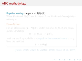
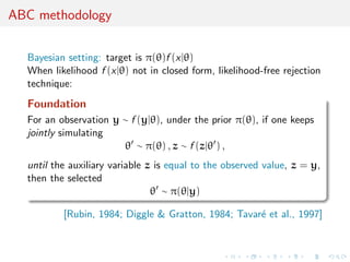
![ABC methodology
Bayesian setting: target is ()f (xj)
When likelihood f (xj) not in closed form, likelihood-free rejection
technique:
Foundation
For an observation y f (yj), under the prior (), if one keeps
jointly simulating
0 () , z f (zj0) ,
until the auxiliary variable z is equal to the observed value, z = y,
then the selected
0 (jy)
[Rubin, 1984; Diggle Gratton, 1984; Tavare et al., 1997]](https://image.slidesharecdn.com/ho1wjotimgbqygqfye1g-signature-8be37557a25ca84b691076eb3d9b0b90d5f3cf9a8a52b597ab20c4e203a597cc-poli-141213034223-conversion-gate01/85/3rd-NIPS-Workshop-on-PROBABILISTIC-PROGRAMMING-29-320.jpg)
![ABC methodology
Bayesian setting: target is ()f (xj)
When likelihood f (xj) not in closed form, likelihood-free rejection
technique:
Foundation
For an observation y f (yj), under the prior (), if one keeps
jointly simulating
0 () , z f (zj0) ,
until the auxiliary variable z is equal to the observed value, z = y,
then the selected
0 (jy)
[Rubin, 1984; Diggle Gratton, 1984; Tavare et al., 1997]](https://image.slidesharecdn.com/ho1wjotimgbqygqfye1g-signature-8be37557a25ca84b691076eb3d9b0b90d5f3cf9a8a52b597ab20c4e203a597cc-poli-141213034223-conversion-gate01/85/3rd-NIPS-Workshop-on-PROBABILISTIC-PROGRAMMING-30-320.jpg)
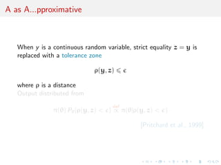
![A as A...pproximative
When y is a continuous random variable, strict equality z = y is
replaced with a tolerance zone
(y, z) 6
where is a distance
Output distributed from
() Pf(y, z) g
def
/ (j(y, z) )
[Pritchard et al., 1999]](https://image.slidesharecdn.com/ho1wjotimgbqygqfye1g-signature-8be37557a25ca84b691076eb3d9b0b90d5f3cf9a8a52b597ab20c4e203a597cc-poli-141213034223-conversion-gate01/85/3rd-NIPS-Workshop-on-PROBABILISTIC-PROGRAMMING-31-320.jpg)
![A as A...pproximative
When y is a continuous random variable, strict equality z = y is
replaced with a tolerance zone
(y, z) 6
where is a distance
Output distributed from
() Pf(y, z) g
def
/ (j(y, z) )
[Pritchard et al., 1999]](https://image.slidesharecdn.com/ho1wjotimgbqygqfye1g-signature-8be37557a25ca84b691076eb3d9b0b90d5f3cf9a8a52b597ab20c4e203a597cc-poli-141213034223-conversion-gate01/85/3rd-NIPS-Workshop-on-PROBABILISTIC-PROGRAMMING-32-320.jpg)
![eld]
I Loss of statistical information balanced against gain in data
roughening
I Approximation error and information loss remain unknown
I Choice of statistics induces choice of distance function
towards standardisation
I may be imposed for external/practical reasons (e.g., DIYABC)
I may gather several non-B point estimates [the more the
merrier]
I can [machine-]learn about ecient combination](https://image.slidesharecdn.com/ho1wjotimgbqygqfye1g-signature-8be37557a25ca84b691076eb3d9b0b90d5f3cf9a8a52b597ab20c4e203a597cc-poli-141213034223-conversion-gate01/85/3rd-NIPS-Workshop-on-PROBABILISTIC-PROGRAMMING-38-320.jpg)
![eld]
I Loss of statistical information balanced against gain in data
roughening
I Approximation error and information loss remain unknown
I Choice of statistics induces choice of distance function
towards standardisation
I may be imposed for external/practical reasons (e.g., DIYABC)
I may gather several non-B point estimates [the more the
merrier]
I can [machine-]learn about ecient combination](https://image.slidesharecdn.com/ho1wjotimgbqygqfye1g-signature-8be37557a25ca84b691076eb3d9b0b90d5f3cf9a8a52b597ab20c4e203a597cc-poli-141213034223-conversion-gate01/85/3rd-NIPS-Workshop-on-PROBABILISTIC-PROGRAMMING-40-320.jpg)
![eld]
I Loss of statistical information balanced against gain in data
roughening
I Approximation error and information loss remain unknown
I Choice of statistics induces choice of distance function
towards standardisation
I may be imposed for external/practical reasons (e.g., DIYABC)
I may gather several non-B point estimates [the more the
merrier]
I can [machine-]learn about ecient combination](https://image.slidesharecdn.com/ho1wjotimgbqygqfye1g-signature-8be37557a25ca84b691076eb3d9b0b90d5f3cf9a8a52b597ab20c4e203a597cc-poli-141213034223-conversion-gate01/85/3rd-NIPS-Workshop-on-PROBABILISTIC-PROGRAMMING-42-320.jpg)
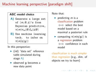
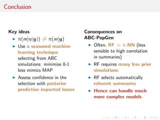
![Machine learning perspective [paradigm shift]
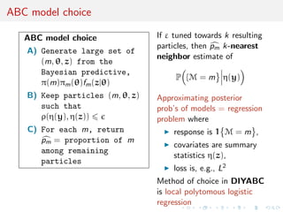
ABC model choice
A) Generate a large set
of (m, , z)'s from
Bayesian predictive,
(m)m()fm(zj)
B) Use machine learning
tech. to infer on
(m](https://image.slidesharecdn.com/ho1wjotimgbqygqfye1g-signature-8be37557a25ca84b691076eb3d9b0b90d5f3cf9a8a52b597ab20c4e203a597cc-poli-141213034223-conversion-gate01/85/3rd-NIPS-Workshop-on-PROBABILISTIC-PROGRAMMING-51-320.jpg)
![cation and regression
[Breiman, 1996]
Improved classi](https://image.slidesharecdn.com/ho1wjotimgbqygqfye1g-signature-8be37557a25ca84b691076eb3d9b0b90d5f3cf9a8a52b597ab20c4e203a597cc-poli-141213034223-conversion-gate01/85/3rd-NIPS-Workshop-on-PROBABILISTIC-PROGRAMMING-61-320.jpg)
![cation schemes of randomly generated training sets, creating
a forest of (CART) decision trees, inspired by Amit and Geman
(1997) ensemble learning
[Breiman, 2001]](https://image.slidesharecdn.com/ho1wjotimgbqygqfye1g-signature-8be37557a25ca84b691076eb3d9b0b90d5f3cf9a8a52b597ab20c4e203a597cc-poli-141213034223-conversion-gate01/85/3rd-NIPS-Workshop-on-PROBABILISTIC-PROGRAMMING-63-320.jpg)
![Growing the forest
Breiman's solution for inducing random features in the trees of the
forest:
I boostrap resampling of the dataset and
I random subset-ing [of size
p
t] of the covariates driving the
classi](https://image.slidesharecdn.com/ho1wjotimgbqygqfye1g-signature-8be37557a25ca84b691076eb3d9b0b90d5f3cf9a8a52b597ab20c4e203a597cc-poli-141213034223-conversion-gate01/85/3rd-NIPS-Workshop-on-PROBABILISTIC-PROGRAMMING-68-320.jpg)

![Subsampling
Due to both large datasets [practical] and theoretical
recommendation of Scornet et al. (2014), from independence
between trees to convergence issues, boostrap sample of much
smaller size than original data size
nboot = o(n)
Each CART tree stops when number of observations per node is 1:
no culling of the branches](https://image.slidesharecdn.com/ho1wjotimgbqygqfye1g-signature-8be37557a25ca84b691076eb3d9b0b90d5f3cf9a8a52b597ab20c4e203a597cc-poli-141213034223-conversion-gate01/85/3rd-NIPS-Workshop-on-PROBABILISTIC-PROGRAMMING-71-320.jpg)
![Subsampling
Due to both large datasets [practical] and theoretical
recommendation of Scornet et al. (2014), from independence
between trees to convergence issues, boostrap sample of much
smaller size than original data size
nboot = o(n)
Each CART tree stops when number of observations per node is 1:
no culling of the branches](https://image.slidesharecdn.com/ho1wjotimgbqygqfye1g-signature-8be37557a25ca84b691076eb3d9b0b90d5f3cf9a8a52b597ab20c4e203a597cc-poli-141213034223-conversion-gate01/85/3rd-NIPS-Workshop-on-PROBABILISTIC-PROGRAMMING-72-320.jpg)
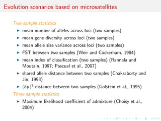
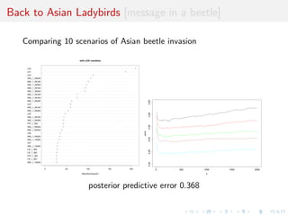
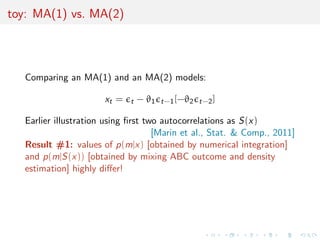
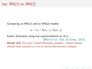
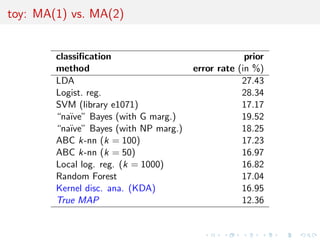
![toy: MA(1) vs. MA(2)
Comparing an MA(1) and an MA(2) models:
xt = t - #1t-1[-#2t-2]
Earlier illustration using](https://image.slidesharecdn.com/ho1wjotimgbqygqfye1g-signature-8be37557a25ca84b691076eb3d9b0b90d5f3cf9a8a52b597ab20c4e203a597cc-poli-141213034223-conversion-gate01/85/3rd-NIPS-Workshop-on-PROBABILISTIC-PROGRAMMING-86-320.jpg)
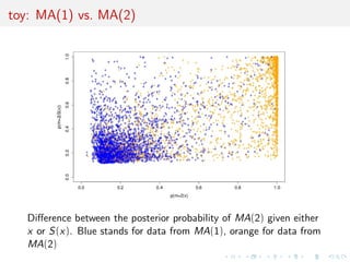
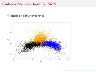
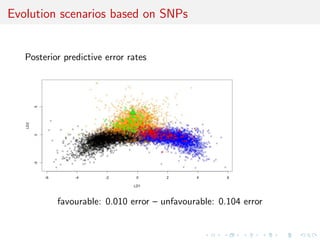
![rst two autocorrelations as S(x)
[Marin et al., Stat. Comp., 2011]
Result #1: values of p(mjx) [obtained by numerical integration]
and p(mjS(x)) [obtained by mixing ABC outcome and density
estimation] highly dier!](https://image.slidesharecdn.com/ho1wjotimgbqygqfye1g-signature-8be37557a25ca84b691076eb3d9b0b90d5f3cf9a8a52b597ab20c4e203a597cc-poli-141213034223-conversion-gate01/85/3rd-NIPS-Workshop-on-PROBABILISTIC-PROGRAMMING-87-320.jpg)
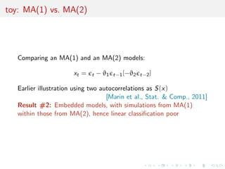
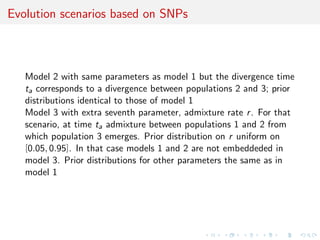
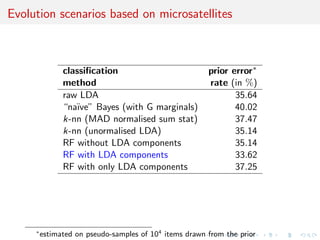
![toy: MA(1) vs. MA(2)
Comparing an MA(1) and an MA(2) models:
xt = t - #1t-1[-#2t-2]
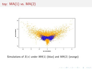
Earlier illustration using two autocorrelations as S(x)
[Marin et al., Stat. Comp., 2011]
Result #2: Embedded models, with simulations from MA(1)
within those from MA(2), hence linear classi](https://image.slidesharecdn.com/ho1wjotimgbqygqfye1g-signature-8be37557a25ca84b691076eb3d9b0b90d5f3cf9a8a52b597ab20c4e203a597cc-poli-141213034223-conversion-gate01/85/3rd-NIPS-Workshop-on-PROBABILISTIC-PROGRAMMING-89-320.jpg)

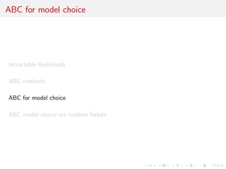
This document discusses approximate Bayesian computation (ABC) methods for performing Bayesian inference when the likelihood function is intractable. ABC methods approximate the posterior distribution by simulating data under different parameter values and selecting simulations that match the observed data based on summary statistics. The document outlines how ABC originated in population genetics to model complex demographic scenarios and mutation processes. It then describes the basic ABC rejection sampling algorithm and how it provides an approximation of the posterior distribution by sampling from regions of high density defined by the summary statistics.


![[A]BCel : a presentation at ABC in Roma](https://cdn.slidesharecdn.com/ss_thumbnails/abcel-130530042650-phpapp02-thumbnail.jpg?width=640&height=640&fit=bounds)


![Columbia workshop [ABC model choice]](https://cdn.slidesharecdn.com/ss_thumbnails/columbia-110924060002-phpapp01-thumbnail.jpg?width=640&height=640&fit=bounds)


