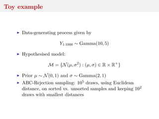
Downloaded 10 times
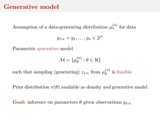
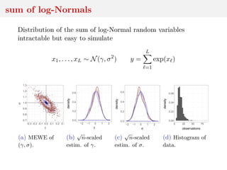
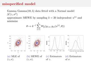
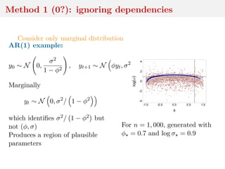
![Summary statistics
Since random variable y1:n − z1:n may have large variance,
{ y1:n − z1:n < ε}
gets rare as ε → 0 and rarer when d ↑
When using
|η(y1:n) − η(z1:n) < ε
based on (insufficient) summary statistic η, variance and
dimension decrease but q-likelihood differs from likelihood
Arbitrariness and impact of summaries, incl. curse of
dimensionality
[X et al., 2011; Fearnhead & Prangle, 2012; Li & Fearnhead, 2016]](https://image.slidesharecdn.com/inewton-180827214101/85/ABC-with-Wasserstein-distances-6-320.jpg)
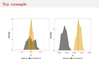

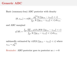
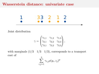
![Wasserstein distance
Ground distance ρ (x, y) → ρ(x, y) on Y along with order p ≥ 1
leads to Wasserstein distance between µ, ν ∈ Pp(Y), p ≥ 1:
Wp(µ, ν) = inf
γ∈Γ(µ,ν) Y×Y
ρ(x, y)p
dγ(x, y)
1/p
where Γ(µ, ν) set of joints with marginals µ, ν and Pp(Y) set of
distributions µ for which Eµ[ρ(Y, y0)p] < ∞ for one y0](https://image.slidesharecdn.com/inewton-180827214101/85/ABC-with-Wasserstein-distances-13-320.jpg)
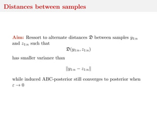
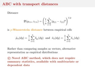
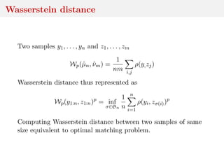
![Wasserstein distance
Two samples y1, . . . , yn and z1, . . . , zm
Wp(ˆµn, ˆνm) =
1
nm i,j
ρ(y,zj)
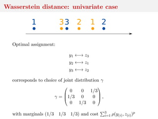
Important special case when n = m, for which solution to the
optimization problem γ corresponds to an assignment matrix,
with only one non-zero entry per row and column, equal to n−1.
[Villani, 2003]](https://image.slidesharecdn.com/inewton-180827214101/85/ABC-with-Wasserstein-distances-17-320.jpg)
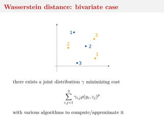
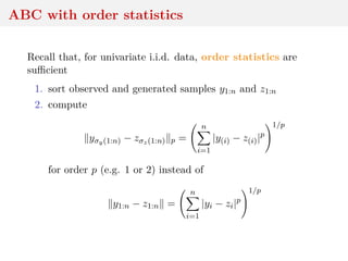
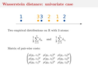
![Wasserstein distance
also called Earth Mover, Gini, Mallows, Kantorovich, &tc.
can be defined between arbitrary distributions
actual distance
statistically sound:
ˆθn = arginf
θ∈H
Wp(
1
n
n
i=1
δyi , µθ) → θ = arginf
θ∈H
Wp(µ , µθ),
at rate
√
n, plus asymptotic distribution
[Bassetti & al., 2006]](https://image.slidesharecdn.com/inewton-180827214101/85/ABC-with-Wasserstein-distances-20-320.jpg)


![Computing Wasserstein distances
when Y = R, computing Wp(µn, νn) costs O(n log n)
when Y = Rd, exact calculation is O(n3) [Hungarian]or
O(n2.5 log n) [short-list]
For entropic regularization, with δ > 0
Wp,δ(ˆµn, ˆνn)p
= inf
γ∈Γ(ˆµn,ˆνn) Y×Y
ρ(x, y)p
dγ(x, y) − δH(γ) ,
where H(γ) = − ij γij log γij entropy of γ, existence of
Sinkhorn’s algorithm that yields cost O(n2)
[Genevay et al., 2016]](https://image.slidesharecdn.com/inewton-180827214101/85/ABC-with-Wasserstein-distances-23-320.jpg)
![Computing Wasserstein distances
other approximations, like Ye et al. (2016) using Simulated
Annealing
regularized Wasserstein not a distance, but as δ goes to
zero,
Wp,δ(ˆµn, ˆνn) → Wp(ˆµn, ˆνn)
for δ small enough, Wp,δ(ˆµn, ˆνn) = Wp(ˆµn, ˆνn) (exact)
in practice, δ 5% of median(ρ(yi, zj)p)i,j
[Cuturi, 2013]](https://image.slidesharecdn.com/inewton-180827214101/85/ABC-with-Wasserstein-distances-24-320.jpg)
![Computing Wasserstein distances
cost linear in the dimension of
observations
distance calculations
model-independent
other transport distances
calculated in O(n log n), based
on different generalizations of
“sorting” (swapping, Hilbert)
[Gerber & Chopin, 2015]
acceleration by combination of
distances and subsampling
[source: Wikipedia]](https://image.slidesharecdn.com/inewton-180827214101/85/ABC-with-Wasserstein-distances-25-320.jpg)
![Computing Wasserstein distances
cost linear in the dimension of
observations
distance calculations
model-independent
other transport distances
calculated in O(n log n), based
on different generalizations of
“sorting” (swapping, Hilbert)
[Gerber & Chopin, 2015]
acceleration by combination of
distances and subsampling
[source: Wikipedia]](https://image.slidesharecdn.com/inewton-180827214101/85/ABC-with-Wasserstein-distances-26-320.jpg)
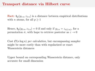
![Transport distance via Hilbert curve
Sort multivariate data via space-filling curves, like Hilbert
space-filling curve
H : [0, 1] → [0, 1]d
continuous mapping, with pseudo-inverse
h : [0, 1]d
→ [0, 1]
Compute order σ ∈ S of projected points, and compute
hp(y1:n, z1:n) =
1
n
n
i=1
ρ(yσy(i), zσz(i))p
1/p
,
called Hilbert ordering transport distance
[Gerber & Chopin, 2015]](https://image.slidesharecdn.com/inewton-180827214101/85/ABC-with-Wasserstein-distances-27-320.jpg)
![Adaptive SMC with r-hit moves
Start with ε0 = ∞
1. ∀k ∈ 1 : N, sample θk
0 ∼ π(θ) (prior)
2. ∀k ∈ 1 : N, sample zk
1:n from µ
(n)
θk
3. ∀k ∈ 1 : N, compute the distance dk
0 = D(y1:n, zk
1:n)
4. based on (θk
0)N
k=1 and (dk
0)N
k=1, compute ε1, s.t.
resampled particles have at least 50% unique values
At step t ≥ 1, weight wk
t ∝ 1(dk
t−1 ≤ εt), resample, and perform
r-hit MCMC with adaptive independent proposals
[Lee, 2012; Lee and Latuszy´nski, 2014]](https://image.slidesharecdn.com/inewton-180827214101/85/ABC-with-Wasserstein-distances-29-320.jpg)
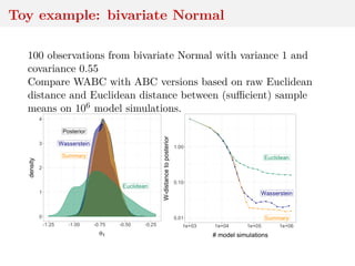
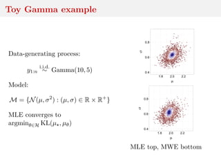
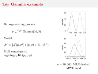
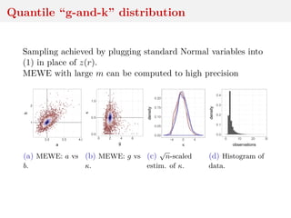
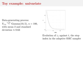
![Quantile “g-and-k” distribution
bivariate extension of the g-and-k distribution with quantile
functions
ai + bi 1 + 0.8
1 − exp(−gizi(r)
1 + exp(−giz(r)
1 + zi(r)2
k
zi(r) (1)
and correlation ρ
Intractable density that can be numerically approximated
[Rayner and MacGillivray, 2002; Prangle, 2017]
Simulation by MCMC and W-ABC (sequential tolerance
exploration)](https://image.slidesharecdn.com/inewton-180827214101/85/ABC-with-Wasserstein-distances-31-320.jpg)
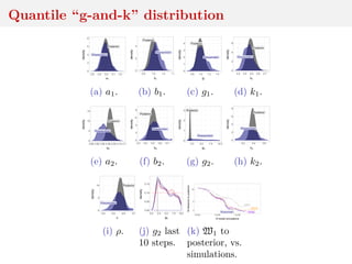

![Minimum Wasserstein estimator
Under stronger assumptions, incl. well-specification,
dim(Y) = 1, and p = 1
√
n(ˆθn − θ )
w
−→ argmin
u∈H R
|G (t) − u, D (t) |dt,
where G is a µ -Brownian bridge, and D ∈ (L1(R))dθ satisfies
R
|Fθ(t) − F (t) − θ − θ , D (t) |dt = o( θ − θ H)
[Pollard, 1980; del Barrio et al., 1999, 2005]
Hard to use for confidence intervals, but the bootstrap is an
intersting alternative.](https://image.slidesharecdn.com/inewton-180827214101/85/ABC-with-Wasserstein-distances-35-320.jpg)
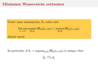
![Minimum expected Wasserstein estimator
ˆθn,m = argmin
θ∈H
E[D(ˆµn, ˆµθ,m)]
with expectation under distribution of sample z1:m ∼ µ
(m)
θ
giving rise to ˆµθ,m = m−1 m
i=1 δzi .](https://image.slidesharecdn.com/inewton-180827214101/85/ABC-with-Wasserstein-distances-38-320.jpg)
![Minimum expected Wasserstein estimator
ˆθn,m = argmin
θ∈H
E[D(ˆµn, ˆµθ,m)]
with expectation under distribution of sample z1:m ∼ µ
(m)
θ
giving rise to ˆµθ,m = m−1 m
i=1 δzi .
Under further assumptions, incl. m(n) → ∞ with n,
inf
θ∈H
EWp(ˆµn(ω), ˆµθ,m(n)) → inf
θ∈H
Wp(µ , µθ)
and
lim sup
n→∞
argmin
θ∈H
EWp(ˆµn(ω), ˆµθ,m(n)) ⊂ argmin
θ∈H
Wp(µ , µθ).](https://image.slidesharecdn.com/inewton-180827214101/85/ABC-with-Wasserstein-distances-39-320.jpg)
![Minimum expected Wasserstein estimator
ˆθn,m = argmin
θ∈H
E[D(ˆµn, ˆµθ,m)]
with expectation under distribution of sample z1:m ∼ µ
(m)
θ
giving rise to ˆµθ,m = m−1 m
i=1 δzi .
Further, for n fixed,
inf
θ∈H
EWp(ˆµn, ˆµθ,m) → inf
θ∈H
Wp(ˆµn, µθ)
as m → ∞ and
lim sup
m→∞
argmin
θ∈H
EWp(ˆµn, ˆµθ,m) ⊂ argmin
θ∈H
Wp(ˆµn, µθ).](https://image.slidesharecdn.com/inewton-180827214101/85/ABC-with-Wasserstein-distances-40-320.jpg)
![Asymptotics of WABC-posterior
convergence to true posterior as → 0
convergence to non-Dirac as n → ∞ for fixed
Bayesian consistency if n ↓ at proper speed
[Frazier, X & Rousseau, 2017]](https://image.slidesharecdn.com/inewton-180827214101/85/ABC-with-Wasserstein-distances-42-320.jpg)
![Asymptotics of WABC-posterior
convergence to true posterior as → 0
convergence to non-Dirac as n → ∞ for fixed
Bayesian consistency if n ↓ at proper speed
[Frazier, X & Rousseau, 2017]
WARNING: Theoretical conditions extremely rarely open
checks in practice](https://image.slidesharecdn.com/inewton-180827214101/85/ABC-with-Wasserstein-distances-43-320.jpg)
![Asymptotics of WABC-posterior
For fixed n and ε → 0, for i.i.d. data, assuming
sup
y,θ
µθ(y) < ∞
y → µθ(y) continuous, the Wasserstein ABC-posterior converges
to the posterior irrespective of the choice of ρ and p
Concentration as both n → ∞ and ε → ε = inf Wp(µ , µθ)
[Frazier et al., 2018]
Concentration on neighborhoods of θ = arginf Wp(µ , µθ),
whereas posterior concentrates on arginf KL(µ , µθ)](https://image.slidesharecdn.com/inewton-180827214101/85/ABC-with-Wasserstein-distances-44-320.jpg)
![Asymptotics of WABC-posterior
Rate of posterior concentration (and choice of εn) relates to
rate of convergence of the distance, e.g.
µ
(n)
θ Wp µθ,
1
n
n
i=1
δzi > u ≤ c(θ)fn(u),
[Fournier & Guillin, 2015]
Rate of convergence decays with the dimension of Y,](https://image.slidesharecdn.com/inewton-180827214101/85/ABC-with-Wasserstein-distances-45-320.jpg)
![Asymptotics of WABC-posterior
Rate of posterior concentration (and choice of εn) relates to
rate of convergence of the distance, e.g.
µ
(n)
θ Wp µθ,
1
n
n
i=1
δzi > u ≤ c(θ)fn(u),
[Fournier & Guillin, 2015]
Rate of convergence decays with the dimension of Y, fast or
slow, depending on moments of µθ and choice of p](https://image.slidesharecdn.com/inewton-180827214101/85/ABC-with-Wasserstein-distances-46-320.jpg)
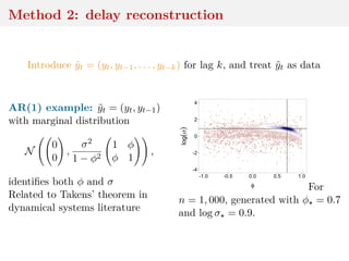
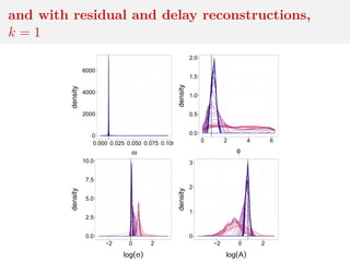
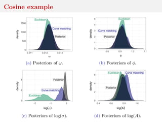
![Method 3: residual reconstruction
Time series y1:n deterministic transform of θ and w1:n
Given y1:n and θ, reconstruct w1:n
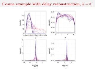
Cosine example:
yt = A cos(2πωt + φ) + σwt
wt ∼ N(0, 1)
wt = (yt − A cos(2πωt + φ))/σ
and calculate distance between
reconstructed w1:n and Normal
sample
[Mengersen et al., 2013]](https://image.slidesharecdn.com/inewton-180827214101/85/ABC-with-Wasserstein-distances-57-320.jpg)
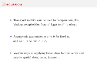
![Method 3: residual reconstruction
Time series y1:n deterministic transform of θ and w1:n
Given y1:n and θ, reconstruct w1:n
Cosine example:
yt = A cos(2πωt + φ) + σwt
n = 500 observations with
ω = 1/80, φ = π/4,
σ = 1, A = 2, under prior
U[0, 0.1] and U[0, 2π] for ω and φ,
and N(0, 1) for log σ, log A
−2.5
0.0
2.5
0 100 200 300 400 500
time
y](https://image.slidesharecdn.com/inewton-180827214101/85/ABC-with-Wasserstein-distances-58-320.jpg)

This document discusses using the Wasserstein distance for inference in generative models. It begins by introducing ABC methods that use a distance between samples to compare observed and simulated data. It then discusses using the Wasserstein distance as an alternative distance metric that has lower variance than the Euclidean distance. The document covers computational aspects of calculating the Wasserstein distance, asymptotic properties of minimum Wasserstein estimators, and applications to time series data.

![[DL輪読会]Convolutional Conditional Neural Processesと Neural Processes Familyの紹介](https://cdn.slidesharecdn.com/ss_thumbnails/20191220readingpaperconvcnp-191220034420-thumbnail.jpg?width=640&height=640&fit=bounds)


![[DL輪読会]Deep Neural Networks as Gaussian Processes](https://cdn.slidesharecdn.com/ss_thumbnails/dl0216okamoto2162-180323031830-thumbnail.jpg?width=640&height=640&fit=bounds)


![Inference in generative models using the Wasserstein distance [[INI]](https://cdn.slidesharecdn.com/ss_thumbnails/inewton-170706120746-thumbnail.jpg?width=640&height=640&fit=bounds)


![ANIMAL_CELL_,_TISSUE_AND_ORGAN_CULTURE[1].pptx](https://cdn.slidesharecdn.com/ss_thumbnails/animalcelltissueandorganculture1-260204172026-4462b440-thumbnail.jpg?width=640&height=640&fit=bounds)


