Intro to Approximate Bayesian Computation (ABC)

An intro to ABC – approximate Bayesian
computation
PhD course FMS020F–NAMS002 “Statistical inference for partially
observed stochastic processes”, Lund University
http://goo.gl/sX8vU9
Umberto Picchini
Centre for Mathematical Sciences,
Lund University
www.maths.lth.se/matstat/staff/umberto/
Umberto Picchini (umberto@maths.lth.se)

In this lecture we consider the case where it is not possible to pursue
exact inference for model parameters θ, nor it is possible to
approximate the likelihood function of θ within a given computational
budget and available time.
The above is not a rare circumstance.
Since the advent of affordable computers and the introduction of
advanced statistical methods, researchers have become increasingly
ambitious, and try to formulate and ﬁt very complex models.
Example: MCMC (Markov chain Monte Carlo) has provided a
universal machinery for Bayesian inference since its rediscovery in
the statistical community in the early 90’s.
Thanks to MCMC (and related methods) scientists’ ambitions have
been pushed further and further.

However for complex models (and/or large datasets) MCMC is often
impractical. Calculating the likelihood, or an approximation thereof
might be impossible.
For example in spatial statistics INLA (integrated nested Laplace
approximation) is a welcome alternative to the more expensive
MCMC.
Also MCMC is not online: when new observations arrive we have to
re-compute the whole likelihood for the total set of observations, i.e.
we can’t make use of the likelihood computed at previous
observations.

Particle marginal methods (particle MCMC) are a fantastic possibility
for exact Bayesian inference for state-space models. But what can we
do for non-state space models?
And what can we do when the dimension of the mathematical system
is large and the implementation of particle ﬁlters with millions of
particles is infeasible?

There is an increasingly interest in statistical methods for models that
are easy to simulate from, but for which it is impossible to calculate
transition densities or likelihoods.
General set-up: we have a complex stochastic process {Xt} with
unknown parameters θ. For any θ we can simulate from this process.
We have observations y = f({X0:T}).
We want to estimate θ but we cannot calculate p(y|θ), as this involves
integrating over the realisations of {X0:T}.
Notice we are not specifying the probabilistic properties of X0:T nor
Y. We are certainly not restricting ourselves to state-space models.

The likelihood-free idea
Likelihood-free inference motivating idea:
Easy to simulate from model conditional on parameters.
So run simulations for many parameters.
See for which parameter value the simulated data sets match
observed data best

Different likelihood-free methods
Likelihood-free methods date back to at least Diggle and Gratton
(1984) and Rubin (1984, p. 1160)
More recent examples:
Indirect Inference (Gourieroux and Ronchetti 1993);
Approximate Bayesian Computation (ABC) (a review is Marin
et al. 2011);
bootstrap ﬁlter of Gordon, Salmond and Smith (1993)
Synthetic Likelihoods method of Wood (2010)

Are approximations any worth?
Why should we care about approximate methods?
Well, we know the most obvious answer: it’s because this is what we
do when exact methods are impractical. No big news...
But I am more interested on the following phenomenon, which I
noticed by direct experience:
Many scientists seem to get intellectual fulﬁlment by using exact
methods, leading to exact inference.
What we might not see is when they fail to communicate that
they (consciously or unconsciously) pushed themselves to
formulate simpler models, so that exact inference could be
achieved.

So the pattern I often notice is:
1 You have a complex scenario, noisy data, unobserved variables
etc
2 you formulate a pretty realistic model... which you can’t ﬁt to
data (i.e. exact inference is not possible)
3 you simplify the model (a lot) so it is now tractable with exact
methods.
4 You are happy.
However you might have simpliﬁed the model a wee too much to be
realistic/useful/sound.

John Tukey – 1962
“Far better an approximate answer to the right question, which is
often vague, than an exact answer to the wrong question, which can
always be made precise. ”
If a complex model is the one I want to use to answer the right
question, then I prefer to obtain an approximative answer using
approximate inference, than fooling myself with a simpler model
using exact inference.

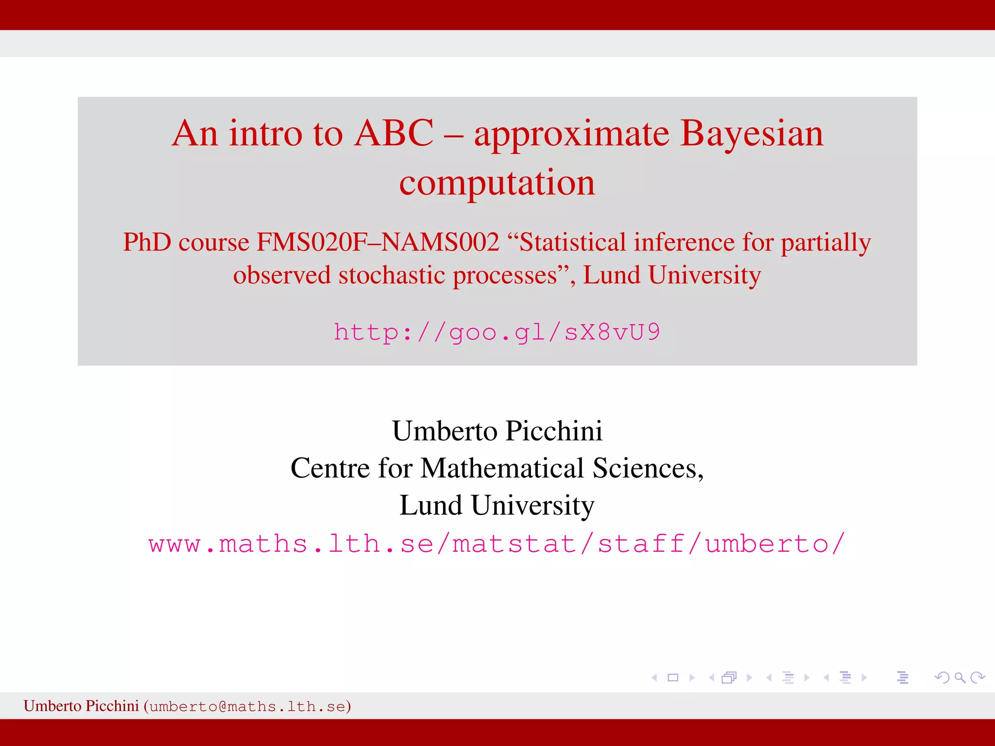
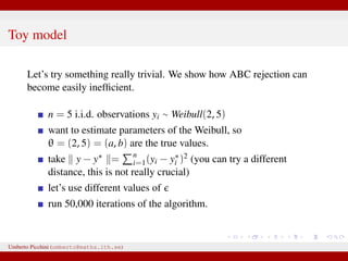
Gelman and Rubin, 1996
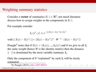
“[...] as emphasized in Rubin (1984), one of the great scientiﬁc
advantages of simulation analysis of Bayesian methods is the freedom
it gives the researcher to formulate appropriate models rather than be
overly interested in analytically neat but scientiﬁcally inappropriate
models.”
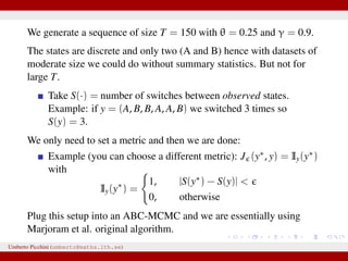
Approximate Bayesian Computation and Synthetic Likelihoods are
two approximate methods for inference, with ABC vastly more
popular and with older origins.
We will discuss ABC only.

Features of ABC
only need a generative model, i.e. the model we assumed having
generated available data y.
only need to be able to simulate from such a model.
in other words, we do not need to assume anything regarding the
probabilistic features of the model components.
particle marginal methods also assume the ability to simulate
from the model, but also assume a speciﬁc model structure,
usually a state-space model (SSM).
also, particle marginal methods for SSM require at least
knowledge of p(yt|xt; θ) (to compute importance weights). What
do we do without such requirement?

For the moment we can denote data with y instead of, say, y1:T as
what we are going to introduce is not speciﬁc to dynamical models.

Bayesian setting: target is π(θ|y) ∝ p(y|θ)π(θ)
What to do when (1) the likelihood p(y|θ) is unknown in closed form
and/or (2) it is expensive to approximate?
Notice that if we are able to simulate observations y∗ by running the
generative model, then we have
y∗
∼ p(y|θ)
That is y∗ is produced by the statistical model that generated observed
data y.
(i) Therefore if Y is the space where y takes values, then y∗ ∈ Y.
(ii) y and y∗ have the same dimension.

Loosely speaking...
Example: if we have a SSM and given a parameter value θ and xt−1
simulate xt, then plug xt in the observation equation ans simulate y∗
t ,
then I have that y∗
t ∼ p(yt|θ).
This is because if I have two random variables x and y with joint
distribution (conditional on θ) p(y, x|θ) then
p(y, x|θ) = p(y|x; θ)p(x|θ).
I ﬁrst simulate x∗ from p(x|θ), then conditional on x∗ I simulate y∗
from p(y|x∗, θ).
What I obtain is a draw (x∗, y∗) from p(y, x|θ) hence y∗ alone must be
a draw from the marginal p(y|θ).

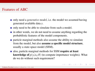
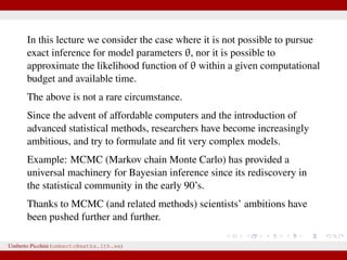
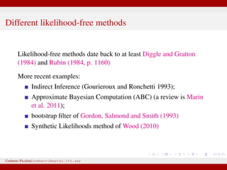
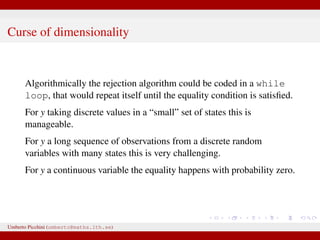
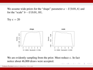
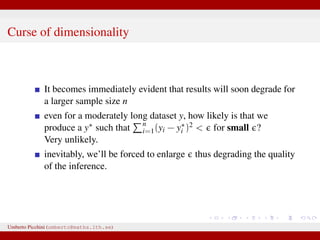
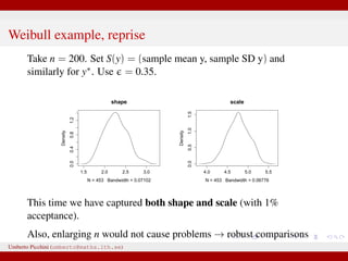
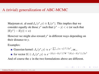
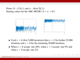
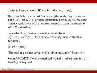
Likelihood free rejection sampling
1 simulate from the prior θ∗ ∼ π(θ)
2 plug θ∗ in your model and simulate a y∗ [this is the same as
writing y∗ ∼ p(y|θ∗)]
3 if y∗ = y store θ∗. Go to step 1 and repeat.
The above is a likelihood free algorithm: it does not require
knowledge of the expression of p(y|θ).
Each accepted θ∗ is such that θ∗ ∼ π(θ|y) exactly.
We justify the result in next slide.

Justiﬁcation
The previous algorithm is exact. Let’s see why.
Denote with f(θ∗, y∗) the joint distribution of the accepted (θ∗, y∗).
We have that
f(θ∗
, y∗
) = p(y∗
|θ∗
)π(θ∗
)Iy(y∗
)
with Iy(y∗) = 1 iff y∗ = y and zero otherwise. Marginalizing y∗ we
have
f(θ∗
) =
Y
p(y∗
|θ∗
)π(θ∗
)Iy(y∗
)dy∗
= p(y|θ∗
)π(θ∗
) ∝ π(θ∗
|y)
hence all accepted θ∗ are drawn from the exact posterior.

Curse of dimensionality
Algorithmically the rejection algorithm could be coded in a while
loop, that would repeat itself until the equality condition is satisﬁed.
For y taking discrete values in a “small” set of states this is
manageable.
For y a long sequence of observations from a discrete random
variables with many states this is very challenging.
For y a continuous variable the equality happens with probability zero.

ABC rejection sampling (Tavare et al.1
)
Attack the curse of dimensionality by introducing an approximation.
Take an arbitrary distance · and a threshold > 0.
2 simulate a y∗ ∼ p(y|θ∗)
3 if y∗ − y < store θ∗. Go to step 1 and repeat.
Each accepted θ∗ is such that θ∗ ∼ π (θ|y).
π (θ|y) ∝
Y
p(y∗
|θ∗
)π(θ∗
)IA ,y (y∗
)dy∗
A ,y(y∗) = {y∗ ∈ Y; y∗ − y < }.
1
Tavare et al. 1997. Genetics;145(2)

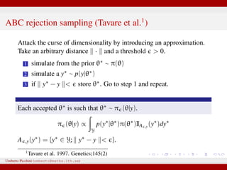
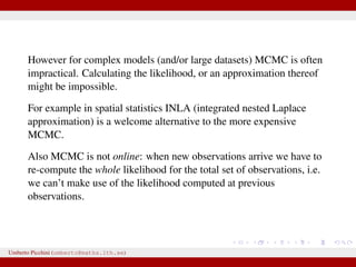
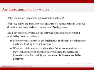
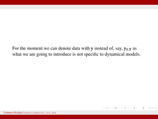
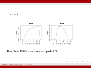
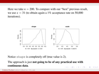
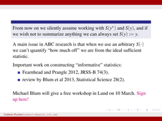
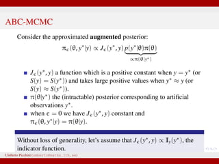
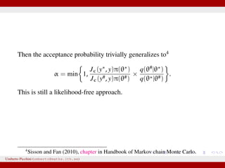
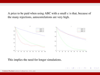
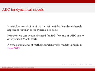
Step 5: The posterior distribution is approximated with the
accepted parameter points. The posterior distribution should have
a nonnegligible probability for parameter values in a region
This example application of ABC used simplifications for
illustrative purposes. A number of review articles provide pointers
to more realistic applications of ABC [9–11,14].
Figure 1. Parameter estimation by Approximate Bayesian Computation: a conceptual overview.
doi:10.1371/journal.pcbi.1002803.g001

It is self evident that when imposing = 0 we force y∗ = y thus
implying that draws will be, again, from the true posterior.
However in practice imposing = 0 might require unbearable
computational times to obtain a single acceptance. In practice we
have to set > 0, so that draws are from the approximate posterior
π (θ|y).
Important ABC result
Convergence “in distribution”:
when → 0, π (θ|y) → π(θ|y)
when → ∞, π (θ|y) → π(θ)
Essentially for a too large we learn nothing.

Toy model
Let’s try something really trivial. We show how ABC rejection can
become easily inefﬁcient.
n = 5 i.i.d. observations yi ∼ Weibull(2, 5)
want to estimate parameters of the Weibull, so
θ = (2, 5) = (a, b) are the true values.
take y − y∗ = n
i=1(yi − y∗
i )2 (you can try a different
distance, this is not really crucial)
let’s use different values of
run 50,000 iterations of the algorithm.

We assume wide priors for the “shape” parameter a ∼ U(0.01, 6) and
for the “scale” b ∼ U(0.01, 10).
Try = 20
0 1 2 3 4 5 6
0.000.050.100.15
shape
N = 45654 Bandwidth = 0.1699
Density
0 2 4 6 8 10
0.000.040.08
scale
N = 45654 Bandwidth = 0.3038
Density
We are evidently sampling from the prior. Must reduce . In fact
notice about 46,000 draws were accepted.

Try = 7
0 1 2 3 4 5 6
0.000.100.20
shape
N = 19146 Bandwidth = 0.1779
Density
0 2 4 6 8 10
0.000.050.100.150.20
scale
N = 19146 Bandwidth = 0.2186
Density
Here about 19,000 draws were accepted (38%).

Try = 3
0 2 4 6
0.000.100.20 shape
N = 586 Bandwidth = 0.321
Density
2 4 6 8 10
0.00.10.20.30.4
scale
N = 586 Bandwidth = 0.2233
DensityHere about 1% of the produced simulations has been accepted. Recall
true values are (a, b) = (2, 5).
Of course n = 5 is a very small sample size so inference is of limited
quality, but you got the idea of the method.

An idea for self-study
Compare the ABC (marginal) posteriors with exact posteriors from
some experiment using conjugate priors.
For example see http://www.johndcook.com/
CompendiumOfConjugatePriors.pdf

Curse of dimensionality
It becomes immediately evident that results will soon degrade for
a larger sample size n
even for a moderately long dataset y, how likely is that we
produce a y∗ such that n
i=1(yi − y∗
i )2 < for small ?
Very unlikely.
inevitably, we’ll be forced to enlarge thus degrading the quality
of the inference.

Here we take n = 200. To compare with our “best” previous result,
we use = 31 (to obtain again a 1% acceptance rate on 50,000
iterations).
3.0 3.5 4.0 4.5 5.0 5.5 6.0 6.5
0.00.20.40.60.8
shape
N = 474 Bandwidth = 0.1351
Density
3.5 4.0 4.5 5.0 5.5
0.00.40.81.2
scale
N = 474 Bandwidth = 0.08315
Density
Notice shape is completely off (true value is 2).
The approach is just not going to be of any practical use with
continuous data.

ABC rejection with summaries (Pritchard et al.2
)
Same as before, but comparing S(y) with S(y∗) for “appropriate”
summary statistics S(·).
2 simulate a y∗ ∼ p(y|θ∗), compute S(y∗)
3 if S(y∗) − S(y) < store θ∗. Go to step 1 and repeat.
Samples are from π (θ|S(y)) with
π (θ|S(y)) ∝
Y
p(y∗
|θ∗
)π(θ∗
)IA ,y (y∗
)dy∗
A ,y(y∗) = {y∗ ∈ Y; S(y∗) − S(y) < }.
2
Pritchard et al. 1999, Molecular Biology and Evolution, 16:1791-1798.

Using summary statistics clearly introduces a further level of
approximation. Except when S(·) is sufficient for θ (carries the same
info about θ as the whole y).
When S(·) is a set of sufficient statistics for θ,
π (θ|S(y)) = π (θ|y)
But then again when y is not in the exponential family, we basically
have no hope to construct sufficient statistics.
A central topic in ABC is to construct “informative” statistics, as
a replacement for the (unattainable) sufficient ones.
Important paper, Fearnhead and Prangle 2012 (discussed later).
If we have “good summaries” we can bypass the curse of
dimensionality problem.

Weibull example, reprise
Take n = 200. Set S(y) = (sample mean y, sample SD y) and
similarly for y∗. Use = 0.35.
1.5 2.0 2.5 3.0
0.00.40.81.2
shape
N = 453 Bandwidth = 0.07102
Density
4.0 4.5 5.0 5.5
0.00.51.01.5
scale
N = 453 Bandwidth = 0.06776Density
This time we have captured both shape and scale (with 1%
acceptance).
Also, enlarging n would not cause problems → robust comparisons
thanks to S(·).Umberto Picchini (umberto@maths.lth.se)

From now on we silently assume working with S(y∗) and S(y), and if
we wish not to summarize anything we can always set S(y) := y.
A main issue in ABC research is that when we use an arbitrary S(·)
we can’t quantify “how much off” we are from the ideal sufﬁcient
statistic.
Important work on constructing “informative” statistics:
Fearnhead and Prangle 2012, JRSS-B 74(3).
review by Blum et al 2013, Statistical Science 28(2).
Michael Blum will give a free workshop in Lund on 10 March. Sign
up here!

Beyond ABC rejection
ABC rejection is the simplest example of ABC algorithm.
It generates independent draws and can be coded into an
embarrassingly parallel algorithm. However in can be massively
inefﬁcient.
Parameters are proposed from the prior π(θ). A prior does not exploit
the information of already accepted parameters.
Unless π(θ) is somehow similar to π (θ|y) many proposals will be
rejected for moderately small .
This is especially true for a large dimensional θ.
A natural approach is to consider ABC within an MCMC algorithm.
In a MCMC with random walk proposals the proposed parameter
explores a neighbourhood of the last accepted parameter.

ABC-MCMC
Consider the approximated augmented posterior:
π (θ, y∗
|y) ∝ J (y∗
, y) p(y∗
|θ)π(θ)
∝π(θ|y∗)
J (y∗, y) a function which is a positive constant when y = y∗ (or
S(y) = S(y∗)) and takes large positive values when y∗ ≈ y (or
S(y) ≈ S(y∗)).
π(θ|y∗) the (intractable) posterior corresponding to artiﬁcial
observations y∗.
when = 0 we have J (y∗, y) constant and
π (θ, y∗|y) = π(θ|y).
Without loss of generality, let’s assume that J (y∗, y) ∝ Iy(y∗), the
indicator function.

ABC-MCMC (Marjoram et al. 3
)
We wish to simulate from the posterior π (θ, y∗
|y): hence construct
proposals for both θ and y∗
.
Present state is θ#
(and corresponding y#
). Propose θ∗
∼ q(θ∗
|θ#
).
Simulate y∗
from the model given θ∗
hence the proposal is the model
itself, y∗
∼ p(y∗
|θ∗
).
The acceptance probability is thus:
α = min 1,
Iy(y∗
)p(y∗
|θ∗
)π(θ∗
)
1 × p(y#|θ)π(θ#)
×
q(θ#
|θ∗
)p(y#
|θ#
)
q(θ∗|θ#)p(y∗|θ∗)
The “1” at the denominator it’s there because of course we must start the
algorithm at some admissible (accepted) y#
, hence the denominator will
always have Iy(y#
) = 1.
3
Marjoram et al. 2003, PNAS 100(26).

By considering the simpliﬁcation in the previous acceptance
probability we have the ABC-MCMC:
1 Last accepted parameter is θ# (and corresponding y#). Propose
θ∗ ∼ q(θ∗|θ#).
2 generate y∗ conditionally on θ∗ and compute Iy(y∗)
3 if Iy(y∗) = 1 go to step 4 else stay at θ# and return to step 1.
4 Calculate
α = min 1,
π(θ∗)
π(θ#)
×
q(θ#|θ∗)
q(θ∗|θ#)
generate u ∼ U(0, 1). If u < α set θ# := θ∗ otherwise stay at θ#.
Return to step 1.
During the algorithm there is no need to retain the generated y∗ hence
the set of accepted θ form a Markov chain with stationary distribution
π (θ|y).

The previous ABC-MCMC algorithm is also denoted as
“likelihood-free MCMC”.
Notice that likelihoods do not appear in the algorithm.
Likelihoods are substituted by sampling of artiﬁcial observations
from the data-generating model.
The Handbook of MCMC (CRC press) has a very good chapter
on Likelihood-free Markov chain Monte Carlo.

Blackboard: proof that the algorithm targets the correct distribution

A (trivial) generalization of ABC-MCMC
Marjoram et. al used J (y∗, y) ≡ Iy(y∗). This implies that we
consider equally ok those y∗ such that |y∗ − y| < (or such that
|S(y∗) − S(y)| < )
However we might also reward y∗ in different ways depending on
their distance to y.
Examples:
Gaussian kernel: J (y∗, y) ∝ e− n
i=1(yi−y∗
i )2/2 2
, or...
for vector S(·): J (y∗, y) ∝ e−(S(y)−S(y∗)) W−1(S(y)−S(y∗))/2 2
And of course the in the two formulations above are different.

Then the acceptance probability trivially generalizes to4
α = min 1,
J (y∗, y)π(θ∗)
J (y#, y)π(θ#)
×
q(θ#|θ∗)
q(θ∗|θ#)
.
This is still a likelihood-free approach.
4
Sisson and Fan (2010), chapter in Handbook of Markov chain Monte Carlo.

Choice of the threshold
We would like to use a “small” > 0, however it turns out that if you
start at a bad value of θ a small will cause many rejections.
start with a fairly large allowing the chain to move in the
parameters space.
after some iterations reduce so the chain will explore a
(narrower) and more precise approximation to π(θ|y)
keep reducing (slowly) . Use the set of θ’s accepted using the
smallest to report inference results.
It’s not obvious how to determine the sequence of
1 > 2 > ... > k > 0. If the sequence decreases too fast there will
be many rejections (chain suddenly trapped in some tail).
It’s a problem similar to tuning the “temperature” in optimization via
simulated annealing.

Choice of the threshold
A possibility:
Say that you have completed a number of iterations via ABC-MCMC
or via rejection sampling using 1, and say that you stored the
distances d 1
= S(y) − S(y∗
) obtained using 1.
Take the xth percentile of such distances and set a new threshold 2 as
2 := xth percentile of d 1
.
this way 2 < 1. So now you can use 2 to conduct more simulations,
then similarly obtain 3 := xth percentile of d 2
etc.
Depending on x the decrease from a to another will be more or
less fast. Setting say x = 20 will cause a sharp decrease, while x = 90
will let the threshold decrease more slowly.
A slow decrease of is safer but implies longer simulations before
reaching acceptable results.
Alternatively just to set the sequence of ’s by trial and error.

When do we stop decreasing ?
Several studies have shown that when using ABC-MCMC obtain
a chain resulting in a 1% acceptance rate (at the smallest ) is a
good compromise between accuracy and computational needs.
This is also my experience.
However recall that a “small” implies many rejections→you’ll
have to run a longer simulation to obtain enough acceptances to
enable inference.
ABC, unlike exact MCMC, does require a small acceptance rate.
This is needed by its own nature as we are not happy to use a
large .
A high acceptance rate denotes that your is way too large and
you are probably sampling from the prior π(θ) (!)

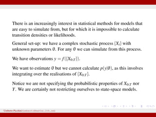
Example from Sunnåker et al. 2013
[Large chunks from the cited article constitute the ABC entry in Wikipedia.]
distribution for these models. Again, computational improvements
for ABC in the space of models have been proposed, such as
constructing a particle filter in the joint space of models and
parameters [17].
Once the posterior probabilities of models have been estimated,
one can make full use of the techniques of Bayesian model
comparison. For instance, to compare the relative plausibilities of
two models M1 and M2, one can compute their posterior ratio,
which is related to the Bayes factor B1,2:
p(M1DD) p(DDM1) p(M1) p(M1)
additional bias due to the loss of information
bias—for example, in the context of mod
more subtle [12,18].
At the same time, some of the criticisms t
at the ABC methods, in particular
phylogeography [19–21], are not specific
all Bayesian methods or even all statistic
choice of prior distribution and param
However, because of the ability of ABC-me
more complex models, some of these g
particular relevance in the context of ABC
This section discusses these potential risk
ways to address them (Table 2).
Approximation of the Posterior
A nonnegligible e comes with the price
p(hDr(^DD,D)ƒe) instead of the true post
sufficiently small tolerance, and a sensible
resulting distribution p(hDr(^DD,D)ƒe) shou
the actual target distribution p(hDD) reasona
hand, a tolerance that is large enough th
parameter space becomes accepted will yiel
distribution. There are empirical studies of
p(hDr(^DD,D)ƒe) and p(hDD) as a function of
results for an upper e-dependent bound for
estimates [24]. The accuracy of the pos
expected quadratic loss) delivered by ABC
also been investigated [25]. However, th
distributions when e approaches zero, and
distance measure used, is an important to
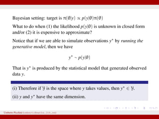
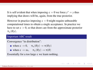
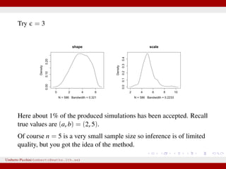
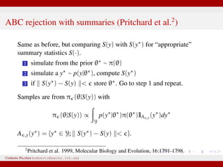
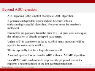
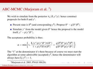
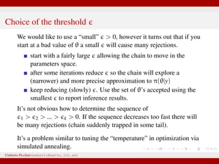
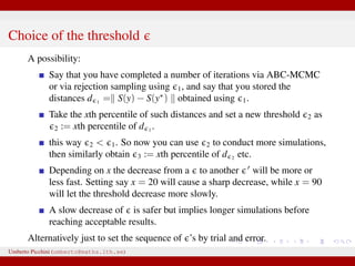
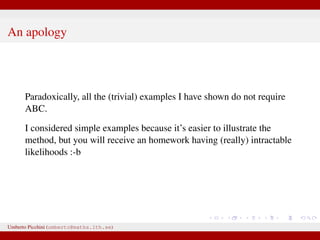
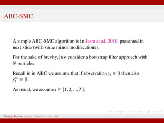
Figure 2. A dynamic bistable hidden Markov model.
doi:10.1371/journal.pcbi.1002803.g002
We have a hidden system state, moving between states {A,B} with
probability θ, and stays in the current state with probability 1 − θ.
Actual observations affected by measurement errors: probability to
misread system states is 1 − γ for both A and B.

Example of application: the behavior of the Sonic Hedgehog (Shh)
transcription factor in Drosophila melanogaster can be modeled by
the given model.
Not surprisingly, the example is a hidden Markov model:
p(xt|xt−1) = θ when xt xt−1 and 1 − θ otherwise.
p(yt|xt) = γ when yt = xt and 1 − γ otherwise.
In other words a typical simulation pattern looks like:
A,B,B,B,A,B,A,A,A,B (states x1:T)
A,A,B,B,B,A,A,A,A,A (observations y1:T)
Misrecorded states are ﬂagged in red.

The example could be certainly solved via exact methods, but just for
the sake of illustration, assume we are only able to simulate random
sequences from our model.
Here is how we simulate a sequence of length T:
1 given θ, generate x∗
t ∼ Bin(1, θ)
2 conditionally on xt, yt is Bernoulli: generate a u ∼ U(0, 1) if
u < γ set y∗
t := x∗
t otherwise take the other value.
3 set t := t + 1 go to 1 and repeat until we have collected y1, ..., yT.
So we are totally set to generate sequences of A’s and B’s given
parameter values.

We generate a sequence of size T = 150 with θ = 0.25 and γ = 0.9.
The states are discrete and only two (A and B) hence with datasets of
moderate size we could do without summary statistics. But not for
large T.
Take S(·) = number of switches between observed states.
Example: if y = (A, B, B, A, A, B) we switched 3 times so
S(y) = 3.
We only need to set a metric and then we are done:
Example (you can choose a different metric): J (y∗, y) = Iy(y∗)
with
Iy(y∗
) =
1, |S(y∗) − S(y)| <
0, otherwise
Plug this setup into an ABC-MCMC and we are essentially using
Marjoram et al. original algorithm.

Priors: θ ∼ U(0, 1) and γ ∼ Beta(20, 3).
Starting values for the ABC-MCMC: θ = γ = 0.5
0 1 2 3 4 5 6 7 8
×104
0
0.2
0.4
0.6
0.8
1
θ
0 1 2 3 4 5 6 7 8
×104
0
0.2
0.4
0.6
0.8
1
γ
Used = 6 (ﬁrst 5,000 iterations) then = 2 for further 25,000
iterations and = 0 for the remaining 50,000 iterations.
When = 6 accept. rate 20%, when = 2 accept. rate 9% and
when = 0 accept. rate 2%.

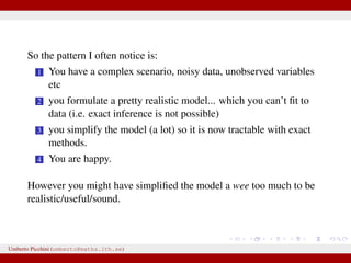
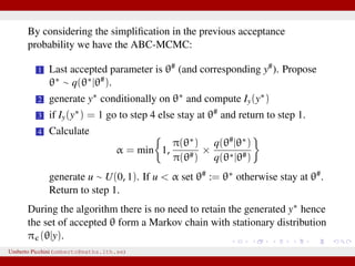
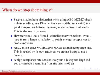
Results at = 0
Dealing with a discrete state-space model allows the luxury to obtain
results at = 0 (impossible with continuous states).
Below: ABC posteriors (blue), true parameters (vertical red lines) and
Beta prior (black). For θ we used a uniform prior in [0,1].
0 0.2 0.4 0.6 0.8 1
0
1
2
3
4
5
θ
0 0.2 0.4 0.6 0.8 1 1.2
0
1
2
3
4
5
6
7
γ
Remember: when using non-sufﬁcient statistics results will be
biased even with = 0.

A price to be paid when using ABC with a small is that, because of
the many rejections, autocorrelations are very high.
0 10 20 30 40 50 60 70 80 90 100
-0.2
0
0.2
0.4
0.6
0.8
1
θ
epsilon = 0
epsilon = 2
epsilon = 6
0 10 20 30 40 50 60 70 80 90 100
0
0.2
0.4
0.6
0.8
1
γ
epsilon = 0
epsilon = 2
epsilon = 6
This implies the need for longer simulations.

An apology
Paradoxically, all the (trivial) examples I have shown do not require
ABC.
I considered simple examples because it’s easier to illustrate the
method, but you will receive an homework having (really) intractable
likelihoods :-b

Weighting summary statistics
Consider a vector of summaries S(·) ∈ Rd, not much literature
discuss how to assign weights to the components in S(·).
For example consider
J (y∗
, y) ∝ e− (S(y)−S(y∗) /2 2
with S(y) − S(y∗) = (S(y) − S(y∗)) · W−1 · (S(y) − S(y∗))
Prangle5 notes that if S(y) = (S1(y), ..., Sd(y)) and if we give to all Sj
the same weight (hence W is the identity matrix) then the distance
· is dominated by the most variable summary Sj.
Only the component of θ “explained” by such Sj will be nicely
estimated.
5
D. Prangle (2015) arXiv:1507.00874

Useful to have a diagonal W, say W = diag(σ2
1, ..., σ2
d).
The σj could be determined from some pilot study. Say that we are
using ABC-MCMC, after some appropriate burnin say that we have
stored R realizations of S(y∗) corresponding to the R parameters θ∗
into a R × d matrix.
For each column j extract the unique values from
(S
(1)
j (y∗), .., S
(R)
j (y∗)) then compute its madj (median absolute
deviation).
Set σ2
j := mad2
j .
(The median absolute deviation is a robust measure of dispersion.)
Rerun ABC-MCMC with the updated W, and an adjustment to will
probably be required.

ABC for dynamical models
It is trickier to select intuitive (i.e. without the Fearnhead-Prangle
approach) summaries for dynamical models.
However, we can bypass the need for S(·) if we use an ABC version
of sequential Monte Carlo.
A very good review of methods for dynamical models is given in
Jasra 2015.

ABC-SMC
A simple ABC-SMC algorithm is in Jasra et al. 2010, presented in
next slide (with some minor modiﬁcations).
For the sake of brevity, just consider a bootstrap ﬁlter approach with
N particles.
Recall in in ABC we assume that if observation yt ∈ Y then also
yi∗
t ∈ Y.
As usual, we assume t ∈ {1, 2, ..., T}.

Step 0.
Set t = 1. For i = 1, ..., N sample xi
1 ∼ π(x0), y∗i
1 ∼ p(y1|xi
1),
compute weights wi
1 = J1, (y1, y∗i
1 ) and normalize weights
˜wi
1 := wi
1/ N
i=1 wi
1.
Step 1.
resample N particles {xi
t, ˜wi
t}. Set wi
t = 1/N.
Set t := t + 1 and if t = T + 1, stop.
Step 2.
For i = 1, ..., N sample xi
t ∼ p(xt|xi
t−1) and y∗i
t ∼ p(yt|xi
t). Compute
wi
t := Jt, (yt, y∗i
t )
normalize weights ˜wi
t := wi
t/ N
i=1 wi
t and go to step 1.

The previous algorithm is not as general as the one actually given in
Jasra et al. 2010.
I assumed that resampling is performed at every t (not strictly
necessary). If resampling is not performed at every t in step 2 we have
wi
t := wi
t−1Jt, (yt, y∗i
t ).
Speciﬁcally Jasra et al. use Jt, (yt, y∗i
t ) ≡ I y∗i
t −yt < but that’s not
essential for the method to work.
What is important to realize is that in SMC methods the comparison
is “local”, that is we compare particles at time t vs. the observation at
t. So we can avoid summaries and use data directly.
That is instead of comparing a length T vector y∗ with a length T
vector y we perform separately T comparisons y∗i
t − yt . This is
very feasible and clearly does not require an S(·).

So you can form an approximation to the likelihood as we explained
in the particle marginal methods lecture, then plug it into a standard
MCMC (not ABC-MCMC) algorithm for parameter estimation.
This is a topic for a ﬁnal project.

Construction of S(·)
We have somehow postponed an important issue in ABC practice: the
choice/construction of S(·).
This is the most serious open-problem in ABC and one often
determining the success or failure of the simulation.
We are ready to accept non-sufﬁciency (available only for data in
the exponential family) in exchange of an “informative statistic”.
Statistics are somehow easier to identify for static models. For
dynamical models their identiﬁcation is rather arbitrary, but see
Martin et al6 for state space models.
6
Martin et al. 2014, arXiv:1409.8363.

Semi-automatic summary statistics
To date the most important study on the construction of summaries in ABC
is in Fearnehad-Prangle 20127
which is a discussion paper on JRSS-B.
Recall a well-known result: consider the class of quadratic losses
L(θ0, ˆθ; A) = (θ0 − ˆθ)T
A(θ0 − ˆθ)
with θ0 true value of a parameter and ˆθ an estimator of θ. A is a positive
deﬁnite matrix.
If we set S(y) = E(θ | y) then the minimal expected quadratic loss
E(L(θ0, ˆθ; A) | y) is achieved via ˆθ = EABC(θ | S(y)) as → 0.
That is to say, as → 0, we minimize the expected posterior loss using the
ABC posterior expectation (if S(y) = E(θ|y)). However E(θ | y) is
unknown.
7
Fearnhead and Prangle (2012).

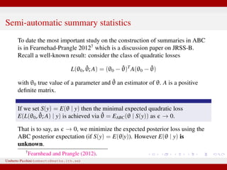
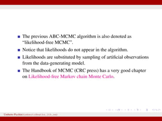
So Fearnhead & Prangle propose a regression-based approach to
determine S(·) (prior to ABC-MCMC start):
for the jth parameter in θ fit separately the linear regression
models
Sj(y) = Ê(θj|y) = ˆβ
(j)
0 + ˆβ(j)
η(y), j = 1, 2, ..., dim(θ)
[e.g. Sj(y) = ˆβ
(j)
0 + ˆβ(j)η(y) = ˆβ
(j)
0 + ˆβ
(j)
1 y0 + · · · + ˆβ
(j)
n yn or
you can let η(·) contain powers of y, say η(y, y2, y3, ...)]
repeat the fitting separately for each θj.
hopefully Sj(y) = ˆβ
(j)
0 + ˆβ(j)η(y) will be “informative” for θj.
Clearly, in the end we have as many summaries as the number of
unknown parameters dim(θ).

An example (run before ABC-MCMC):
1. p = dim(θ). Simulate from the prior θ∗
∼ π(θ) (not very efﬁcient...)
2. using θ∗
, generate y∗
from your model.
Repeat (1)-(2) many times to get the following matrices:




θ
(1)
1 θ
(1)
2 · · · θ
(1)
p
θ
(2)
1 θ
(2)
2 · · · θ
(2)
p
...



 ,




y
∗(1)
1 y
(∗1)
2 · · · y
(∗1)
n
y
(∗2)
1 y
(∗2)
2 · · · y
(∗2)
n
...
... · · ·
...




and for each column of the left matrix do a multivariate linear regression (or
lasso, or...)




θ
(1)
j
θ
(2)
j
...



 =




1 y
(∗1)
1 y
(∗1)
2 · · · y
(∗1)
n
1 y
(∗2)
1 y
(∗2)
2 · · · y
(∗2)
n
...
... · · ·
...



 × βj (j = 1, ..., p),
and obtain a statistic for θj, Sj(·) = ˆβ
(j)
0 + ˆβ(j)
η(·).

Use the same coefﬁcients when calculating summaries for simulated
data and actual data, i.e.
Sj(y) = ˆβ
(j)
0 + ˆβ(j)
η(y)
Sj(y∗
) = ˆβ
(j)
0 + ˆβ(j)
η(y∗
)
In Picchini 2013 I used this approach to select summaries for
state-space models deﬁned by stochastic differential equations.

Software (coloured links are clickable)
EasyABC, R package. Research article.
abc, R package. Research article
abctools, R package. Research article. Focusses on tuning.
Lists with more options here and here .
examples with implemented model simulators (useful to
incorporate in your programs).

Reviews
Fairly extensive but accessible reviews:
1 Sisson and Fan 2010
2 (with applications in ecology) Beaumont 2010
3 Marin et al. 2010
Simpler introductions:
1 Sunnåker et al. 2013
2 (with applications in ecology) Hartig et al. 2013
Review speciﬁc for dynamical models:
1 Jasra 2015

Non-reviews, speciﬁc for dynamical models
1 SMC for Parameter estimation and model comparison: Toni et
al. 2009
2 Markov models: White et al. 2015
3 SMC: Sisson et al. 2007
4 SMC: Dean et al. 2014
5 SMC: Jasra et al. 2010
6 MCMC: Picchini 2013

More specialistic resources
selection of summary statistics: Fearnhead and Prangle 2012.
review on summary statistics selection: Blum et al. 2013
expectation-propagation ABC: Barthelme and Chopin 2012
Gaussian Processes ABC: Meeds and Welling 2014
ABC model choice: Pudlo et al 2015

Blog posts and slides
1 Christian P. Robert often blogs about ABC (and beyond: it’s a
fantastic blog!)
2 an intro to ABC by Darren J. Wilkinson
3 Two posts by Rasmus Bååth here and here
4 Tons of slides at Slideshare.

Intro to Approximate Bayesian Computation (ABC)

Recommended

Recommended

More Related Content

What's hot

What's hot (20)

Similar to Intro to Approximate Bayesian Computation (ABC)

Similar to Intro to Approximate Bayesian Computation (ABC) (20)

Recently uploaded

Recently uploaded (20)

Intro to Approximate Bayesian Computation (ABC)