This document introduces model-based image processing and provides an overview of its key concepts and techniques. It describes model-based image processing as using mathematical and statistical models of images to perform tasks like restoration, reconstruction, and analysis. The document outlines several approaches readers can take to learn model-based image processing, such as understanding probability and estimation, Gaussian and non-Gaussian models, optimization methods, and specific applications like segmentation.


![1.1 What is Model-Based Image Processing? 5
Figure 1.3: Graphical illustration of how forward and prior models can interact syn-
ergistically to dramatically improve results. The green curve represents the thin
manifold in which real images lie, and the gray line represents the thin manifold
defined by noisy linear measurements. If the number of measurements, M, is less
than the number of unknowns, N, then classical methods admit no unique solution.
However, in this case model-based approaches can still provide a useful and unique
solution at the intersection of the measurement and prior manifolds.
visual parallel to the argument that a monkey randomly hitting the keys of a
typewriter would eventually (almost surely in fact) produce Hamlet. While
this may be true, we know that from a practical perspective any given white-
noise image (or random sequence typed by a monkey) is much more likely
to appear to be incoherent noise than a great work of art. This argument
motivates the belief that real natural images have a great deal of structure
that can be usefully exploited when solving inverse problems.
In fact, it can be argued that real natural images fall on thin manifolds in
their embedded space. Such a thin image manifold is illustrated graphically
in Figure 1.3 as a blurry green curve. So if X ∈ [0, 1]N
is an image with
N pixels each of which fall in the interval Xs ∈ [0, 1], then with very high
probability, X will fall within a very small fraction of the space in [0, 1]N
.
Alternatively, a random sample from [0, 1]N
will with virtual certainty never
look like a natural image. It will simply look like noise.
In order to see that a natural images lives on a thin manifold, consider an](https://image.slidesharecdn.com/s6hfi7xht12wwcizuy0v-mbip-book-230123055619-8f2fce45/85/MBIP-book-pdf-15-320.jpg)
![6 Introduction
image with one missing pixel, Xs. Then the conditional distribution of that
pixel given the rest of the image is p(xs|xr r 6= s). In practice, a single missing
pixel from a natural image can almost always be predicted with very high
certainty. Say for example, that µs = E[xs|xr r 6= s] is the conditional mean
of Xs and σs = Std[xs|xr r 6= s] is the conditional standard deviation. Then
the “thickness” the manifold at the location Xr r 6= s is approximately σs.
Since Xs can be predicted with high certainty, we know that σs << 1, and the
manifold is thin at that point. This in turn proves that a manifold containing
real images, as illustrated in green, is thin in most places. However, while
it is thin, it does in fact have some small thickness because we can almost
never predict the missing pixel with absolute certainty. The situation is
illustrated in Figure 1.3 for the case of a 2-D “image” formed by only two
pixels X = [X1, X2].
Measurements typically constrain the solutions of an inverse problem to lie
on a manifold that is, of course, data dependent. If the measurement is linear,
then this thin measurement manifold is approximately a linear manifold (i.e.,
an affine subspace) except it retains some thickness due to the uncertainty
introduced by measurement noise. So let Y = AX + W, where Y is an M
dimensional column vector of measurements, W is the measurement noise,
and A is an M×N matrix. Then each row of A represents a vector, illustrated
by the red vectors of Figure 1.3, that projects X onto a measurement space.
The resulting thin measurement manifold shown in gray is orthogonal to this
projection, and its thickness is determined by the uncertainty due to noise in
the measurement.
If the number of measurements, M, is less than the dimension of the image,
N, then it would seem that the inverse problem can not be meaningfully
solved because the solution can lie anywhere on the thin manifold defined
by the measurement. In this situation, the prior information is absolutely
essential because it effectively reduces the dimensionality of the unknown, X.
Figure 1.3 shows that even when the number of measurements is less than
the number of unknowns, a good solution can be found at the intersection of
the measurement and prior manifolds. This is why model-based methods can
be so powerful in real problems. They allow one to solve inverse problems
that otherwise would have no solution.2
2
Of course, other methods, most notably regularized inversion, have existed for a long time that allow for
the solution of so-called ill-posed inverse problems. In fact, we include these approaches under the umbrella](https://image.slidesharecdn.com/s6hfi7xht12wwcizuy0v-mbip-book-230123055619-8f2fce45/85/MBIP-book-pdf-16-320.jpg)

![8 Introduction
reconstruction error due to blur and other forms of excessive smoothing, or
systematic artifacts such as streaks or offsets.
Figure 1.4 graphically illustrates the tradeoff between variance and bias as
a convex curve.3
As the bias is reduced, the variance must increase. The best
solution depends on the specific application, but, for example, the minimum
mean squared error solution occurs at the interaction of the red curve with
a line of slope -1.
The example of Figure 1.4 illustrates a case where the variance can go
to infinity as the bias goes to zero. In this case, a prior model is essential
to achieving any useful solution. However, the prior model also introduces
some systematic bias in the result; so the crucial idea is to use a prior model
that minimizes any bias that is introduced. Traditional models that assume,
for example, that images are band limited, are not the best models of real
images in most applications, so they result in suboptimal results, such as the
one illustrated with a star. These solutions are suboptimal because at a fixed
bias, there exists a solution with less variance, and at a fixed variance, there
exists a solution with lower bias.
Figure 1.5 shows the practical value of model-based methods [74]. This
result compares state-of-the-art direct reconstruction results and model-based
iterative reconstruction (MBIR) applied to data obtained from a General
Electric 64 slice Volumetric Computed Tomography (VCT) scanner. The
dramatic reduction in noise could not simply be obtained by post-processing
of the image. The increased resolution and reduced noise is the result of the
synergistic interaction between the measured data and the prior model.
1.2 How can I learn Model-Based Image Processing?
The remainder of this book presents the key mathematical and probabilistic
techniques and theories that comprise model-based image processing. Per-
haps the two most critical components are models of both systems and im-
ages, and estimators of X based on those models. In particular, accurate
image models are an essential component of model-based image processing
due to the need to accurately model the thin manifold on which real images
3
It can be proved that the optimal curve must be convex by randomizing the choice of any two algorithms
along the curve.](https://image.slidesharecdn.com/s6hfi7xht12wwcizuy0v-mbip-book-230123055619-8f2fce45/85/MBIP-book-pdf-18-320.jpg)


![14 Probability, Estimation, and Random Processes
where P{X ≤ t} is the probability of the event that X is less than or equal
to t. In fact, F(t) is a valid CDF if and only if it has three properties:
First, it must be a monotone increasing function of t; second, it must be
right hand continuous; and third, must have limits of limt→∞ F(t) = 1 and
limt→−∞ F(t) = 0.
If F(t) is an absolutely continuous function, then it will have an associated
probability density function (PDF), p(t), such that
F(t) =
Z t
−∞
p(τ)dτ .
For most physical problems, it is reasonable to assume that such a density
function exists, and when it does then it is given by
p(t) =
dF(t)
dt
.
Any function1
of a random variable is itself a random variable. So for
example, if we define the new random variable Y = g(X) where g : R → R,
then Y will also be a random variable.
Armed with the random variable X and its distribution, we may define
the expectation as
E[X] ,
Z ∞
−∞
τdF(τ) =
Z ∞
−∞
τp(τ)dτ .
The first integral form is known as a Lebesgue-Stieltjes integral and is
defined even when the probability density does not exist. However, the second
integral containing the density is perhaps more commonly used.
The expectation is a very basic and powerful tool which exists under very
general conditions.2
An important property of expectation, which directly
results from its definition as an integral, is linearity.
Property 2.1. Linearity of expectation - For all random variables X and Y ,
E[X + Y ] = E[X] + E[Y ] .
1
Technically, this can only be a Lebesgue-measurable function; but in practice, measurability is a reason-
able assumption in any physically meaningful situation.
2
In fact, for any positive random variable, X, the E[X] takes on a well-defined value on the extended
real line of (−∞, ∞]. In addition, whenever E[|X|] < ∞, then E[X] is real valued and well-defined. So we
will generally assume that E[|X|] < ∞ for all random variables we consider.](https://image.slidesharecdn.com/s6hfi7xht12wwcizuy0v-mbip-book-230123055619-8f2fce45/85/MBIP-book-pdf-24-320.jpg)
![2.1 Random Variables and Expectation 15
Of course, it is also possible to specify the distribution of groups of random
variables. So let X1, · · · , Xn be n random variables. Then we may specify
the joint distribution of these n random variables via the n-dimensional CDF
given by
F(t1, · · · , tn) = P{X1 ≤ t1, · · · , Xn ≤ tn} .
In this case, there is typically an associated n-dimensional PDF, p(t1, · · · , tn),
so that
F(t1, · · · , tn) =
Z t1
−∞
· · ·
Z tn
−∞
p(τ1, · · · , τn)dτ1 · · · dτn .
Again, any function of the vector X = (X1, · · · , Xn) is then a new random
variable. So for example, if Y = g(X) where g : Rn
→ R, then Y is a random
variable, and we may compute its expectation as
E[Y ] =
Z
Rn
g(τ1, · · · , τn)p(τ1, · · · , τn)dτ1 · · · dτn .
If we have a finite set of random variables, X1, · · · , Xn, then we say the
random variables are jointly independent if we can factor the CDF (or
equivalently the PDF if it exists) into a product with the form,
F(t1, · · · , tn) = Fx1
(t1) · · · Fxn
(tn) ,
where Fxk
(tk) denotes the CDF for the random variable Xk. This leads to
another important property of expectation.
Property 2.2. Expectation of independent random variables - If X1, · · · , Xn
are a set of jointly independent random variables, then we have that
E
" n
Y
k=1
Xk
#
=
n
Y
k=1
E[Xk] .
So when random variables are jointly independent, then expectation and
multiplication can be interchanged. Perhaps surprisingly, pair-wise indepen-
dence of random variables does not imply joint independence. (See problem 3)
One of the most subtle and important concepts in probability is condi-
tional probability and conditional expectation. Let X and Y be two random
variables with a joint CDF given by F(x, y) and marginal CDF given by](https://image.slidesharecdn.com/s6hfi7xht12wwcizuy0v-mbip-book-230123055619-8f2fce45/85/MBIP-book-pdf-25-320.jpg)
![16 Probability, Estimation, and Random Processes
Fy(y) = limx→∞ F(x, y) . The conditional CDF of X given Y = y is then
any function, F(x|y), which solves the equation
F(x, y) =
Z y
−∞
F(x|t)dFy(t) .
At least one solution to this equation is guaranteed to exist by an application
of the famous Radon-Nikodym theorem.3
So the conditional CDF, F(x|y),
is guaranteed to exist. However, this definition of the conditional CDF is
somewhat unsatisfying because it does not specify how to construct F(x|y).
Fortunately, the conditional CDF can be calculated in most practical sit-
uations as
F(x|y) =
dF(x, y)
dy
dF(∞, y)
dy
−1
.
More typically, we will just work with probability density functions so that
p(x, y) =
d2
F(x, y)
dxdy
py(y) =
dF(∞, y)
dy
.
Then the PDF of X given Y = y is given by
p(x|y) =
p(x, y)
py(y)
.
We may now ask what is the conditional expectation of X given Y ? It
will turn out that the answer to this question has a subtle twist because Y
is itself a random variable. Formally, the conditional expectation of X given
Y is given by4
E[X|Y ] =
Z ∞
−∞
xdF(x|Y ) ,
or alternatively using the conditional PDF, it is given by
E[X|Y ] =
Z ∞
−∞
xp(x|Y )dx .
3
Interestingly, the solution is generally not unique, so there can be many such functions F(x|y). However,
it can be shown that if F(x|y) and F′
(x|y) are two distinct solution, then the functions F(x|Y ) and F′
(x|Y )
are almost surely equal.
4
In truth, this is an equality between two random variables that are almost surely equal.](https://image.slidesharecdn.com/s6hfi7xht12wwcizuy0v-mbip-book-230123055619-8f2fce45/85/MBIP-book-pdf-26-320.jpg)
![2.1 Random Variables and Expectation 17
Notice that in both cases, the integral expression for E[X|Y ] is a function of
the random variable Y . This means that the conditional expectation is itself
a random variable!
The fact that the conditional expectation is a random variable is very
useful. For example, consider the so-called indicator function denoted by
IA(X) ,
1 if X ∈ A
0 otherwise
.
Using the indicator function, we may express the conditional probability of
an event, {X ∈ A}, given Y as
P{X ∈ A|Y } = E[IA(X)|Y ] . (2.1)
Conditional expectation also has many useful properties. We list some
below.
Property 2.3. Filtration property of conditional expectation - For all random
variables X, Y , and Z
E[ E[X|Y, Z] |Y ] = E[X|Y ] .
A special case of the filtration property is that E[X] = E[ E[X|Y ]]. This
can be a useful relationship because sometimes it is much easier to evaluate
an expectation in two steps, by first computing E[X|Z] and then taking
the expectation over Z. Another special case of filtration occurs when we
use the relationship of equation (2.1) to express conditional expectations as
conditional probabilities. In this case, we have that
E[ P {X ∈ A|Y, Z} |Y ] = P {X ∈ A|Y } .
Again, this relationship can be very useful when trying to compute condi-
tional expectations.
Property 2.4. Conditional expectation of known quantities - For all random
variables X, Y , and Z, and for all functions f(·)
E[f(X)Z|X, Y ] = f(X)E[Z|X, Y ] ,
which implies that E[X|X, Y ] = X.](https://image.slidesharecdn.com/s6hfi7xht12wwcizuy0v-mbip-book-230123055619-8f2fce45/85/MBIP-book-pdf-27-320.jpg)
![18 Probability, Estimation, and Random Processes
This property states the obvious fact that if we are given knowledge of
X, then the value of f(X) is known. For example, if we are told that the
temperature outside is exactly 100 degrees Fahrenheit, then we know that
the expectation of the outside temperature is 100 degrees Fahrenheit. Notice
that since E[X|Y ] = f(Y ) for some function f(·), Property 2.4 may be used
to show that
E[E[X|Y ] |Y, Z] = E[f(Y )|Y, Z]
= f(Y )
= E[X|Y ] .
Therefore, we know that for all random variables, X, Y , and Z
E[ E[X|Y, Z] |Y ] = E[X|Y ] = E[ E[X|Y ] |Y, Z] . (2.2)
2.2 Some Commonly Used Distributions
Finally, we should introduce some common distributions and their associ-
ated notation. A widely used distribution for a random variable, X, is the
Gaussian distribution denoted by
p(x) =
1
√
2πσ2
exp
−
1
2σ2
(x − µ)2
where µ ∈ R and σ2
0 are known as the mean and variance parameters
of the Gaussian distribution, and it can be easily shown that
E[X] = µ
E
(X − µ)2
= σ2
.
We use the notation X ∼ N(µ, σ2
) to indicate that X is a Gaussian random
variable with mean µ and variance σ2
.
A generalization of the Gaussian distribution is the multivariate Gaus-
sian distribution. We can use vector-matrix notation to compactly repre-
sent the distributions of multivariate Gaussian random vectors. Let X ∈ Rp
denote a p-dimensional random column vector, and Xt
denote its transpose.
Then the PDF of X is given by
p(x) =
1
(2π)p/2
|R|−1/2
exp
−
1
2
(x − µ)t
R−1
(x − µ)
, (2.3)](https://image.slidesharecdn.com/s6hfi7xht12wwcizuy0v-mbip-book-230123055619-8f2fce45/85/MBIP-book-pdf-28-320.jpg)
![2.2 Some Commonly Used Distributions 19
where µ ∈ Rp
is the mean vector and R ∈ Rp×p
is the covariance matrix
of the multivariate Gaussian distribution. Without loss of generality, the
covariance matrix can be assumed to be symmetric (i.e., R = Rt
); however,
in order to be a well defined distribution the covariance must also be positive
definite, otherwise p(x) can not integrate to 1. More precisely, let 0 denote
a column vector of 0’s. We say that a symmetric matrix is positive semi-
definite if for all y ∈ Rp
such that y 6= 0, then ||y||2
R , yt
Ry ≥ 0. If the
inequality is strict, then the matrix is said to be positive definite.
We will use the notation X ∼ N(µ, R) to indicate that X is a multivariate
Gaussian random vector with mean µ and positive-definite covariance R, and
in this case it can be shown that
E[X] = µ
E
(X − µ)(X − µ)t
= R .
A random vector with the distribution of equation (2.3) is also known as a
jointly Gaussian random vector.5
It is important to note that a vector of
Gaussian random variables is not always jointly Gaussian. So for example, it
is possible for each individual random variable to have a marginal distribution
that is Gaussian, but for the overall density not to have the form of (2.3).
Furthermore, it can be shown that a random vector is jointly Gaussian, if and
only if any linear transformation of the vector produces Gaussian random
variables. For example, it is possible to construct two Gaussian random
variables, X1 and X2, such that each individual random variable is Gaussian,
but the sum, Y = X1 + X2, is not. In this case, X1 and X2 are not jointly
Gaussian.
An important property of symmetric matrices is that they can be diagonal-
ized using an orthonormal transformation. So for example, if R is symmetric
and positive definite, then
R = EΛEt
where E is an orthonomal matrix whose columns are the eigenvectors of R
and Λ is a diagonal matrix of strictly positive eigenvalues. Importantly, if
X is a zero-mean Gaussian random vector with covariance R, then we can
5
Furthermore, we say that a finite set of random vectors is jointly Gaussian if the concatenation of these
vectors forms a single vector that is jointly Gaussian.](https://image.slidesharecdn.com/s6hfi7xht12wwcizuy0v-mbip-book-230123055619-8f2fce45/85/MBIP-book-pdf-29-320.jpg)
![20 Probability, Estimation, and Random Processes
decorrelate the entries of the vector X with the transformation
X̃ = Et
X .
In this case, E
h
X̃X̃t
i
= Λ, so the components of the vector X̃ are said to be
uncorrelated since then E
h
X̃iX̃j
i
= 0 for i 6= j. Moreover, it can be easily
proved that since X̃ is jointly Gaussian with uncorrelated components, then
its components must be jointly independent.
Jointly Gaussian random variables have many useful properties, one of
which is listed below.
Property 2.5. Linearity of conditional expectation for Gaussian random vari-
ables - If X ∈ Rn
and Y ∈ Rp
are jointly Gaussian random vectors, then
E[X|Y ] = AY + b
E
(X − E[X|Y ])(X − E[X|Y ])t
|Y
= C ,
where A ∈ Rn×p
is a matrix, b ∈ Rn
is a vector, and C ∈ Rn×n
is a positive-
definite matrix. Furthermore, if X and Y are zero mean, then b = 0 and the
conditional expectation is a linear function of Y .
The Bernoulli distribution is an example of a discrete distribution
which we will find very useful in image and signal modeling applications.
If X has a Bernoulli distribution, then
P{X = 1} = θ
P{X = 0} = 1 − θ ,
where θ ∈ [0, 1] parameterizes the distribution. Since X takes on discrete
values, its CDF has discontinuous jumps. The easiest solution to this problem
is to represent the distribution with a probability mass function (PMF)
rather than a probability density function. The PMF of a random variable or
random vector specifies the actual probability of the random quantity taking
on a specific value. If X has a Bernoulli distribution, then it is easy to show
that its PMF may be expressed in the more compact form
p(x) = (1 − θ)1−x
θx
,
where x ∈ {0, 1}. Another equivalent and sometimes useful expression for
the PMF of a Bernoulli random variable is given by
p(x) = (1 − θ)δ(x − 0) + θδ(x − 1) ,](https://image.slidesharecdn.com/s6hfi7xht12wwcizuy0v-mbip-book-230123055619-8f2fce45/85/MBIP-book-pdf-30-320.jpg)
![2.2 Some Commonly Used Distributions 21
where the function δ(x) is 1 when its argument is 0, and 0 otherwise.
Regardless of the specific choice of distribution, it is often the case that a
series of n experiments are performed with each experiment resulting in an
independent measurement from the same distribution. In this case, we might
have a set of jointly independent random variables, X1, · · · , Xn, which are
independent and identically distributed (i.i.d.). So for example, if the
random variables are i.i.d. Gaussian with distribution N(µ, σ2
), then their
joint distribution is given by
p(x) = p(x1, · · · , xn) =
1
2πσ2
n/2
exp
(
−
1
2σ2
n
X
k=1
(xk − µ)2
)
.
Notice that for notational simplicity, x is used to denote the entire vector of
measurements.
Example 2.1. Let X1, · · · , Xn be n i.i.d. Gaussian random vectors each with
multivariate Gaussian distribution given by N(µ, R), where µ ∈ Rp
and R ∈
Rp
×Rp
. We would like to know the density function for the entire observation.
In order to simplify notation, we will represent the data as a matrix
X = [X1, · · · , Xn] .
Since the n observations, X1, · · · , Xn, are i.i.d., we know we can represent
the density of X as the following product of densities for each vector Xk.
p(x) =
n
Y
k=1
1
(2π)p/2
|R|−1/2
exp
−
1
2
(xk − µ)t
R−1
(xk − µ)
=
1
(2π)np/2
|R|−n/2
exp
(
−
1
2
n
X
k=1
(xk − µ)t
R−1
(xk − µ)
)
This expression may be further simplified by defining the following two new
sample statistics,
b =
n
X
k=1
xk = x1 (2.4)
S =
n
X
k=1
xkxt
k = xxt
, (2.5)](https://image.slidesharecdn.com/s6hfi7xht12wwcizuy0v-mbip-book-230123055619-8f2fce45/85/MBIP-book-pdf-31-320.jpg)

![2.3 Frequentist and Bayesian Estimators 23
2.3 Frequentist and Bayesian Estimators
Once we have decided on a model, our next step is often to estimate some
information from the observed data. There are two general frameworks for
estimating unknown information from data. We will refer to these two general
frameworks as the Frequentist and Bayesian approaches. We will see that
each approach is valuable, and the key is understanding what combination of
approaches is best for a particular application.
The following subsections present each of the two approaches, and then
provide some insight into the strengths and weaknesses of each approach.
2.3.1 Frequentist Estimation and the ML Estimator
In the frequentist approach, one treats the unknown quantity as a determin-
istic, but unknown parameter vector, θ ∈ Ω. So for example, after we observe
the random vector Y ∈ Rp
, then our objective is to use Y to estimate the un-
known scalar or vector θ. In order to formulate this problem, we will assume
that the vector Y has a PDF given by pθ(y) where θ parameterizes a family
of density functions for Y . We may then use this family of distributions to
determine a function, T : Rn
→ Ω, that can be used to compute an estimate
of the unknown parameter as
θ̂ = T(Y ) .
Notice, that since T(Y ) is a function of the random vector Y , the estimate,
θ̂, is a random vector. The mean of the estimator, θ̄, can be computed as
θ̄ = Eθ
h
θ̂
i
= Eθ[T(Y )] =
Z
Rn
T(y)pθ(y)dy .
The difference between the mean of the estimator and the value of the pa-
rameter is known as the bias and is given by
biasθ = θ̄ − θ .
Similarly, the variance of the estimator is given by
varθ = Eθ
θ̂ − θ̄
2
,](https://image.slidesharecdn.com/s6hfi7xht12wwcizuy0v-mbip-book-230123055619-8f2fce45/85/MBIP-book-pdf-33-320.jpg)

![2.3 Frequentist and Bayesian Estimators 25
estimator given by
θ̂ = arg max
θ∈Ω
pθ(Y )
= arg max
θ∈Ω
log pθ(Y ) .
where the notation “arg max” denotes the value of the argument that achieves
the global maximum of the function. Notice that these formulas for the ML
estimate actually use the random variable Y as an argument to the density
function pθ(y). This implies that θ̂ is a function of Y , which in turn means
that θ̂ is a random variable.
When the density function, pθ(y), is a continuously differentiable function
of θ, then a necessary condition when computing the ML estimate is that the
gradient of the likelihood is zero.
∇θ pθ(Y )|θ=θ̂ = 0 .
While the ML estimate is generally not unbiased, it does have a number
of desirable properties. It can be shown that under relatively mild technical
conditions, the ML estimate is both consistent and asymptotically effi-
cient. This means that the ML estimate attains the Cramér-Rao bound
asymptotically as the number of independent data samples, n, goes to infin-
ity [69]. Since this Cramér-Rao bound is a lower bound on the variance of
an unbiased estimator, this means that the ML estimate is about as good as
any unbiased estimator can be. So if one has no idea what values of θ may
occur, and needs to guarantee good performance for all cases, then the ML
estimator is usually a good choice.
Example 2.3. Let {Yk}n
k=1 be i.i.d. random variables with Gaussian distribu-
tion N(θ, σ2
) and unknown mean parameter θ. For this case, the logarithm
of the density function is given by
log pθ(Y ) = −
1
2σ2
n
X
k=1
(Yk − θ)2
−
n
2
log 2πσ2
.
Differentiating the log likelihood results in the following expression.
d log pθ(Y )
dθ θ=θ̂
=
1
σ2
n
X
k=1
(Yk − θ̂) = 0](https://image.slidesharecdn.com/s6hfi7xht12wwcizuy0v-mbip-book-230123055619-8f2fce45/85/MBIP-book-pdf-35-320.jpg)
![26 Probability, Estimation, and Random Processes
From this we obtain the ML estimate for θ.
θ̂ =
1
n
n
X
k=1
Yk
Notice that, by the following argument, this particular ML estimate is unbi-
ased.
Eθ
h
θ̂
i
= Eθ
1
n
n
X
k=1
Yk
#
=
1
n
n
X
k=1
Eθ[Yk] =
1
n
n
X
k=1
θ = θ
Moreover, for this special case, it can be shown that the ML estimator is also
the UMVU estimator [69].
Example 2.4. Again, let X1, · · · , Xn be n i.i.d. Gaussian random vectors each
with multivariate Gaussian distribution given by N(µ, R), where µ ∈ Rp
. We
would like to compute the ML estimate of the parameter vector θ = [µ, R].
Using the statistics b and S from Example 2.1, we can define the sample
mean and covariance given by
µ̂ = b/n (2.8)
R̂ = (S/n) − µ̂µ̂t
, (2.9)
then by manipulation of equation (2.6) the probability distribution of X can
be written in the form
p(x|θ) =
1
(2π)np/2
|R|−n/2
exp
n
−
n
2
tr
n
R̂R−1
o
−
n
2
(µ̂ − µ)t
R−1
(µ̂ − µ)
o
(2.10)
Maximizing this expression with respect to θ then results in the ML estimate
of the mean and covariance given by
arg max
[µ,R]
p(x|µ, R) = [µ̂, R̂] .
So from this we see that the ML estimate of the mean and covariance of a
multivariate Gaussian distribution is simply given by the sample mean and
covariance of the observations.](https://image.slidesharecdn.com/s6hfi7xht12wwcizuy0v-mbip-book-230123055619-8f2fce45/85/MBIP-book-pdf-36-320.jpg)

![28 Probability, Estimation, and Random Processes
The good news with Bayesian estimators is that once we make the as-
sumption that X is random, then the design of estimators is conceptually
straightforward, and the MSE of our estimator can be reduced by estimating
values of X that are more probable to occur. However, the bad news is that
when we assume that X is a random vector, we must select some distribution
for it. In some cases, the distribution for X may be easy to select, but in
many cases, it may be very difficult to select a reasonable distribution or
model for X. And in some cases, a poor choice of this prior distribution can
severely degrade the accuracy of the estimator.
In any case, let us assume that the joint distribution of both Y and X is
known, and let C(x, x̂) ≥ 0 be the cost of choosing x̂ as our estimate if x
is the correct value of the unknown. If our estimate is perfect, then x̂ = x,
which implies that C(x, x̂) = C(x, x) = 0; so the cost is zero. Of course, in
most cases our estimates will not be perfect, so our objective is to select an
estimator that minimizes the expected cost. For a given value of X = x, the
expected cost is given by
C̄(x) = E[C(x, T(Y ))|X = x]
=
Z
Rn
C(x, T(y))py|x(y|x)dy
where py|x(y|x) is the conditional distribution of the data, Y , given the un-
known, X. Here again, the cost is a function of the unknown, X, but we can
remove this dependency by taking the expectation to form what is known as
the Bayes’ risk.
Risk = E[C(X, T(Y ))]
= E[ E[C(X, T(Y ))|X]]
= E
C̄(X)
=
Z
C̄(x)px(x)dx
Notice, that the risk is not a function of X. This stands in contrast to
the Frequentist case, where the MSE of the estimator was a function of θ.
However, the price we pay for removing this dependency is that the risk now
depends critically on the choice of the density function px(x), which specifies
the distribution on the unknown X. The distribution of X is known as the](https://image.slidesharecdn.com/s6hfi7xht12wwcizuy0v-mbip-book-230123055619-8f2fce45/85/MBIP-book-pdf-38-320.jpg)
![2.3 Frequentist and Bayesian Estimators 29
prior distribution since it is the distribution that X is assumed to have
prior to the observation of any data.
Of course, the choice of a specific cost function will determine the form
of the resulting best estimator. For example, it can be shown that when the
cost is squared error, so that C(x, x̂) = |x − x̂|2
, then the optimal estimator
is given by the conditional expectation
X̂MMSE = E[X|Y ] ,
and when the cost is absolute error, so that C(x, x̂) = |x − x̂|, then the
optimal estimator is given by the conditional median.
Z X̂median
−∞
px|y(x|Y )dx =
1
2
Another important case, that will be used extensively in this book, is when
the cost is given by
C(x, x̂) = 1 − δ(x − x̂) =
0 if x = x̂
1 if x 6= x̂
.
Here, the cost is only zero when x = x̂, and otherwise the cost is fixed at
1. This is a very pessimistic cost function since it assigns the same value
whether the error is very small or very large. The optimal estimator for
this cost function is given by the so-called maximum a posteriori (MAP)
estimate,
X̂MAP = arg max
x∈Ω
px|y(x|Y ) , (2.11)
where Ω is the set of feasible values for X, and the conditional distribution
px|y(x|y) is known as the posterior distribution because it specifies the
distribution of the unknown X given the observation Y .
Typically, it is most natural to express the posterior probability in terms
of the forward model, py|x(y|x), and the prior model, px(x), using Bayes’
rule.
px|y(x|y) =
py|x(y|x)px(x)
py(y)
, (2.12)
In practice, the forward model can typically be formulated from a physical
model of how the measurements, Y , are obtained given an assumed image, X.](https://image.slidesharecdn.com/s6hfi7xht12wwcizuy0v-mbip-book-230123055619-8f2fce45/85/MBIP-book-pdf-39-320.jpg)


![32 Probability, Estimation, and Random Processes
Differentiating this expression a second time yields the result that
a = −
1
2
1
σ2
w
+
1
σ2
x
,
and solving for b yields
b =
σ2
x
σ2
x + σ2
w
y .
In fact, looking at the expression of equation (2.17), one can see that the
parameters b and a specify the posterior mean and variance, respectively.
More specifically, if we define µx|y to be the mean of the posterior density
and σ2
x|y to be its variance, then we have the relationships that
−
1
2σ2
x|y
= a = −
1
2
1
σ2
w
+
1
σ2
x
= −
1
2
σ2
w + σ2
x
σ2
wσ2
x
µx|y = b =
σ2
x
σ2
x + σ2
w
y .
Solving for the conditional mean and variance, we can then write an explicit
expression for the conditional distribution of x given y as
px|y(x|y) =
1
q
2πσ2
x|y
exp
(
−
1
2σ2
x|y
(x − µx|y)2
)
, (2.18)
where
µx|y =
σ2
x
σ2
x + σ2
w
y
σ2
x|y =
σ2
xσ2
w
σ2
x + σ2
w
.
While simple, the result of Example 2.6 is extremely valuable in providing
intuition about the behavior of Bayesian estimates. First, from the form of
(2.18), we can easily see that the MMSE estimate of X given Y is given by
X̂MMSE = E[X|Y ] =
σ2
x
σ2
x + σ2
w
Y =
1
1 + σ2
w
σ2
x
Y .](https://image.slidesharecdn.com/s6hfi7xht12wwcizuy0v-mbip-book-230123055619-8f2fce45/85/MBIP-book-pdf-42-320.jpg)
![2.3 Frequentist and Bayesian Estimators 33
Notice that the MMSE estimate is given by Y multiplied by a constant,
0 ≤ σ2
x
σ2
x+σ2
w
1. In other words, the Bayesian estimate is simply an attenuated
version of Y . Moreover, the degree of attenuation is related to the ratio σ2
w/σ2
x,
which is the noise-to-signal ratio. When the noise-to-signal ratio is low,
the attenuation is low because Y is a good estimate of X; but when the
noise-to-signal ratio is high, then the attenuation is great because Y is only
loosely correlated with X. While this attenuation can reduce mean-square
error, it also results in an estimate which is biased because
E
h
X̂MMSE|X
i
=
σ2
x
σ2
x + σ2
w
X X .
This scalar result can also be generalized to the case of jointly Gaussian
random vectors to produce a result of general practical value as shown in the
following example.
Example 2.7. Let X ∼ N(0, Rx) and W ∼ N(0, Rw) be independent Gaus-
sian random vectors, and let Y = X + W. Then the conditional distribution
of X given Y can be calculated in much the same way as it was done for
Example 2.6. The only difference is that the quadratic expressions are gen-
eralized to matrix vector products and quadratic forms. (See problem 13)
Under these more general conditions, the conditional distribution is given by
px|y(x|y) =
1
(2π)p/2
Rx|y
−1/2
exp
−
1
2
(x − µx|y)t
R−1
x|y(x − µx|y)
, (2.19)
where
µx|y = R−1
x + R−1
w
−1
R−1
w y
= I + RwR−1
x
−1
y
= Rx (Rx + Rw)−1
y
Rx|y = R−1
x + R−1
w
−1
= Rx (Rx + Rw)−1
Rw ,
and the MMSE estimate of X given Y is then given by
X̂MMSE = E[X|Y ] = Rx (Rx + Rw)−1
Y . (2.20)](https://image.slidesharecdn.com/s6hfi7xht12wwcizuy0v-mbip-book-230123055619-8f2fce45/85/MBIP-book-pdf-43-320.jpg)
![34 Probability, Estimation, and Random Processes
At this point, there are two interesting observations to make, which are
both particular to the case of jointly Gaussian random variables. First, for
jointly Gaussian random quantities, the posterior mean is a linear function
of the data y, and the posterior variance is not a function of y. These two
properties will not hold for more general distributions. Second, when the
observation, Y , and unknown, X, are jointly Gaussian, then the posterior
distribution is Gaussian, so it is both a symmetric and unimodal function of
x. Therefore, for jointly Gaussian random quantities, the conditional mean,
conditional median, and MAP estimates are all identical.
X̂median = X̂MMSE = X̂MAP
However, for more general distributions, these estimators will differ.
2.3.3 Comparison of the ML and MMSE Estimators
In order to better understand the advantages and disadvantages of Bayesian
estimators, we explore a simple example. Consider the case when X is a
Gaussian random vector with distribution N(0, Rx) and Y is formed by
Y = X + W
where W is a Gaussian random vector with distribution N(0, σ2
wI). So in this
case, Y is formed by adding independent Gaussian noise with variance σ2
w to
the components of the unknown vector X. Furthermore, let us assume that
the covariance of X is formed by
[Rx]i,j =
1
1 + i−j
10
2 , (2.21)
such that σw = 0.75 and the dimension is p = 50. Using this model, we
can generate a pseudo-random vector on a computer from the distribution
of X. (See problem 7) Such a vector is shown in the upper left plot of
Figure 2.1. Notice, that X is a relatively smooth function. This is a result
of our particular choice of the covariance Rx. More specifically, because the
covariance drops off slowly as the |i − j| increases, nearby samples will be
highly correlated, and it is probable (but not certain) that the function will](https://image.slidesharecdn.com/s6hfi7xht12wwcizuy0v-mbip-book-230123055619-8f2fce45/85/MBIP-book-pdf-44-320.jpg)

![36 Probability, Estimation, and Random Processes
0 20 40
−2
0
2
Original Signal, X
0 20 40
−2
0
2
Signal with Noise, Y
0 20 40
−2
0
2
ML Estimate of X
0 20 40
−2
0
2
MMSE Estimate of X
Figure 2.1: This figure illustrates the potential advantage of a Bayesian estimate
versus the ML estimate when the prior distribution is known. The original signal
is sampled from the covariance of (2.21) and white noise is added to produce the
observed signal. In this case, the MMSE estimate is much better than the ML estimate
because it uses prior knowledge about the original signal.
So for each integer n ∈ Z, let Xn be a random variable. Then we say that
Xn is a discrete-time random process.
In order to fully specify the distribution of a random process, it is necessary
to specify the joint distribution of all finite subsets of the random variables.
To do this, we can define the following finite-dimensional distribution
Fm,k(tm, · · · , tk) = P {Xm ≤ tm, Xm+1 ≤ tm+1, · · · , Xk ≤ tk} ,
where m and k are any integers with m ≤ k. The extension theorem
(see for example [79] page 3) guarantees that if the set of finite-dimensional
distributions is consistent for all m, k ∈ Z, then the distribution of the in-
finite dimensional random process is well defined. So the set of all finite
dimensional distributions specify the complete distribution of the random
process. Furthermore, if for all m ≤ k, the vector [Xm, Xm+1, · · · , Xk]T
is
jointly Gaussian, then we say that the Xm is a Gaussian random process.](https://image.slidesharecdn.com/s6hfi7xht12wwcizuy0v-mbip-book-230123055619-8f2fce45/85/MBIP-book-pdf-46-320.jpg)
![2.4 Discrete-Time Random Processes 37
Often it is reasonable to assume that the properties of random processes
do not change over time. Of course, the actual values of the random process
change, but the idea is that the statistical properties of the random process
are invariant. This type of time-invariance of random processes is known as
stationarity. As it turns out, there are different ways to specify stationarity
for a random process. Perhaps the most direct approach is to specify that
the distribution of the random process does not change when it is shifted in
time. This is called strict-sense stationary, and it is defined below.
Definition 1. Strict-Sense Stationary Random Process
A 1-D discrete-time random process Xn is said to be strict-sense sta-
tionary if the finite dimensional distributions of the random process Xn
are equal to the finite dimensional distributions of the random process
Yn = Xn−k for all integers k. This means that
Fm,m+k(t0, t1, · · · , tk) = F0,k(t0, t1, · · · , tk) ,
for all integers m and k ≥ 1 and for all values of t0, t1, · · · , tk ∈ R.
Strict-sense stationarity is quite strong because it depends on verifying
that all finite-dimensional distributions are equal for both the original random
process and its shifted version. In practice, it is much easier to check the
second order properties of a random processes, than it is to check all its
finite-dimensional distributions. To this end, we first define the concept of a
second-order random process.
Definition 2. Second Order Random Process
A 1-D discrete-time random process Xn is said to be a second order
random process if for all n, k ∈ Z, E[|XnXk|] ∞, i.e. all second
order moments are finite.
If a random process is second order, then it has a well defined mean, µn,
and time autocovariance, R(n, k), given by the following expressions.
µn = E[Xn]
R(n, k) = E[(Xn − µn)(Xk − µk)]
Armed with these concepts, we can now give the commonly used definition
of wide-sense stationarity.](https://image.slidesharecdn.com/s6hfi7xht12wwcizuy0v-mbip-book-230123055619-8f2fce45/85/MBIP-book-pdf-47-320.jpg)
![38 Probability, Estimation, and Random Processes
Definition 3. Wide-Sense Stationary Random Process
A 1-D second-order discrete-time random process Xn is said to be
wide-sense stationary if for all n, k ∈ Z, the E[Xn] = µ and
E[(Xn − µ)(Xk − µ)] = R(n−k) where µ is a scalar constant and R(n)
is a scalar function of n.
So a discrete-time random process is wide-sense stationary if its mean is
constant and its time autocovariance is only a function of n−k, the difference
between the two times in question.
Reversibility is another important invariance property which holds when
a strict-sense stationary random process, Xn, and its time-reverse, X−n, have
the same distribution. The formal definition of a reversible random pro-
cess is listed below.
Definition 4. Reversible Random Process
A 1-D discrete-time random process Xn is said to be reversible if its
finite dimensional distributions have the property that
F0,k(t0, t1, · · · , tk) = Fm,m+k(tk, tk−1, · · · , t0) ,
for all integers m and k ≥ 1 and for all values of t0, t1, · · · , tk ∈ R.
Gaussian random processes have some properties which make them easier
to analyze than more general random processes. In particular, the mean and
time autocovariance for a Gaussian random process provides all the informa-
tion required to specify its finite-dimensional distributions. In practice, this
means that the distribution of any Gaussian random process is fully specified
by its mean and autocovariance, as stated in the following property.
Property 2.6. Autocovariance specification of Gaussian random processes -
The distribution of a discrete-time Gaussian random process, Xn, is uniquely
specified by its mean, µn, and time autocovariance, R(n, k).
If a Gaussian random process is also stationary, then we can equivalently
specify the distribution of the random process from its power spectral den-
sity. In fact, it turns out that the power spectral density of a zero-mean
wide-sense stationary Gaussian random process is given by the Discrete-
time Fourier transform (DTFT) of its time autocovariance. More for-
mally, if we define SX(ejω
) to be the expected power spectrum of the signal,](https://image.slidesharecdn.com/s6hfi7xht12wwcizuy0v-mbip-book-230123055619-8f2fce45/85/MBIP-book-pdf-48-320.jpg)
![2.4 Discrete-Time Random Processes 39
Xn, then the Wiener-Khinchin theorem states that for a zero-mean wide-
sense stationary random process the power spectrum is given by the following
expression,
SX(ejω
) =
∞
X
n=−∞
R(n)e−jωn
where the right-hand side of the equation is the DTFT of the time autoco-
variance R(n).
Since the DTFT is an invertible transform, knowing SX(ejω
) is equivalent
to knowing the time autocovariance R(n). Therefore the power spectrum also
fully specifies the distribution of a zero-mean wide-sense stationary Gaussian
random process. The next property summarizes this important result.
Property 2.7. Power spectral density specification of a zero-mean wide-sense
stationary Gaussian random process - The distribution of a wide-sense sta-
tionary discrete-time Gaussian random process, Xn, is uniquely specified by
its power spectral density, SX ejω
.
Finally, we consider reversibility of Gaussian random processes. So if Xn
is a wide-sense stationary Gaussian random process, we can define its time-
reversed version as Yn = X−n. Then by the definition of time autocovariance,
we know that
RY (n) = E[(Yk − µ)(Yk+n − µ)]
= E[(X−k − µ)(X−k−n − µ)]
= E[(Xl+n − µ)(Xl − µ)]
= RX(n)
where l = −k − n, and µ is the mean of both Xn and Yn. From this, we
know that Xn and its time reverse, Yn, have the same autocovariance. By
Property 2.6, this means that Xn and Yn have the same distribution. This
leads to the following property.
Property 2.8. Reversibility of stationary Gaussian random processes - Any
wide-sense stationary Gaussian random process is also strict-sense stationary
and reversible.
Finally, we note that all of these properties, strict-sense stationarity, wide-
sense stationarity, autocovariance, power spectral density, and reversibility](https://image.slidesharecdn.com/s6hfi7xht12wwcizuy0v-mbip-book-230123055619-8f2fce45/85/MBIP-book-pdf-49-320.jpg)
![40 Probability, Estimation, and Random Processes
have natural generalizations in 2-D and higher dimensions. In particular, let
Xs1,s2
be a 2-D discrete-space random process that is wide-sense stationary.
Then its 2-D autocovariance function is given by
R(s1 − r1, s2 − r2) = E[(Xs1,s2
− µ)(Xr1,r2
− µ)] .
where µ = E[Xs1,s2
]. Furthermore, the 2-D power spectral density of Xs1,s2
is
given by
SX(ejω1
, ejω2
) =
∞
X
s1=−∞
∞
X
s2=−∞
R(s1, s2)e−jω1s1−jω2s2
(2.22)
where the right-hand side of this equation is known as the discrete-space
Fourier transform (DSFT) of the 2-D autocovariance. In addition, the 2-D
random process is said to be stationary if Xs1,s2
and Ys1,s2
= Xs1−k1,s2−k2
have
the same distribution for all integers k1 and k2; and the 2-D random process is
said to be reversible if Xs1,s2
and Ys1,s2
= X−s1,−s2
have the same distribution.
Again, it can be shown that 2-D zero-mean wide-sense stationary Gaussian
random processes are always reversible and strict-sense stationary.](https://image.slidesharecdn.com/s6hfi7xht12wwcizuy0v-mbip-book-230123055619-8f2fce45/85/MBIP-book-pdf-50-320.jpg)
![2.5 Chapter Problems 41
2.5 Chapter Problems
1. Let Y be a random variable which is uniformly distributed on the interval
[0, 1]; so that it has a PDF of py(y) = 1 for 0 ≤ y ≤ 1 and 0 otherwise.
Calculate the CDF of Y and use this to calculate both the CDF and
PDF of Z = Y 2
.
2. In this problem, we present a method for generating a random vari-
able, Y , with any valid CDF specified by Fy(t). To do this, let X be
a uniformly distributed random variable on the interval [0, 1], and let
Y = f(X) where we define the function
f(u) = inf{t ∈ R|Fy(t) ≥ u} .
Prove that in the general case, Y has the desired CDF. (Hint: First show
that the following two sets are equal, (−∞, Fy(t)] = {u ∈ R : f(u) ≤ t}.)
3. Give an example of three random variables, X1, X2, and X3 such that
for k = 1, 2, 3, P{Xk = 1} = P{Xk = −1} = 1
2, and such Xk and Xj are
independent for all k 6= j, but such that X1, X2, and X3 are not jointly
independent.
4. Let X be a jointly Gaussian random vector, and let A ∈ RM×N
be a
rank M matrix. Then prove that the vector Y = AX is also jointly
Gaussian.
5. Let X ∼ N(0, R) where R is a p × p symmetric positive-definite matrix.
a) Prove that if for all i 6= j, E[XiXj] = 0 (i.e., Xi and Xj are uncorre-
lated), then Xi and Xj are pair-wise independent.
b) Prove that if for all i, j, Xi and Xj are uncorrelated, then the com-
ponents of X are jointly independent.
6. Let X ∼ N(0, R) where R is a p × p symmetric positive-definite matrix.
Further define the precision matrix, B = R−1
, and use the notation
B =
1/σ2
A
At
C
,
where A ∈ R1×(p−1)
and C ∈ R(p−1)×(p−1)
.](https://image.slidesharecdn.com/s6hfi7xht12wwcizuy0v-mbip-book-230123055619-8f2fce45/85/MBIP-book-pdf-51-320.jpg)
![42 Probability, Estimation, and Random Processes
a) Calculate the marginal density of X1, the first component of X, given
the components of the matrix R.
b) Calculate the conditional density of X1 given all the remaining com-
ponents, Y = [X2, · · · , Xp]t
.
c) What is the conditional mean and covariance of X1 given Y ?
7. Let X ∼ N(0, R) where R is a p × p symmetric positive-definite matrix
with an eigen decomposition of the form R = EΛEt
.
a) Calculate the covariance of X̃ = Et
X, and show that the components
of X̃ are jointly independent Gaussian random variables. (Hint: Use the
result of problem 5 above.)
b) Show that if Y = EΛ1/2
W where W ∼ N(0, I), then Y ∼ N(0, R).
How can this result be of practical value?
8. For each of the following cost functions, find expressions for the minimum
risk Bayesian estimator, and show that it minimizes the risk over all
estimators.
a) C(x, x̂) = |x − x̂|2
.
b) C(x, x̂) = |x − x̂|
9. Let {Yi}n
i=1 be i.i.d. Bernoulli random variables with distribution
P {Yi = 1} = θ
P {Yi = 0} = 1 − θ
Compute the ML estimate of θ.
10. Let {Xi}n
i=1 be i.i.d. random variables with distribution
P{Xi = k} = πk
where
Pm
k=1 πk = 1. Compute the ML estimate of the parameter vector
θ = [π1, · · · , πm]. (Hint: You may use the method of Lagrange multipli-
ers to calculate the solution to the constrained optimization.)
11. Let X1, · · · , Xn be i.i.d. random variables with distribution N(µ, σ2
).
Calculate the ML estimate of the parameter vector (µ, σ2
).](https://image.slidesharecdn.com/s6hfi7xht12wwcizuy0v-mbip-book-230123055619-8f2fce45/85/MBIP-book-pdf-52-320.jpg)
![2.5 Chapter Problems 43
12. Let X1, · · · , Xn be i.i.d. Gaussian random vectors with distribution N(µ, R)
where µ ∈ Rp
and R ∈ Rp×p
is a symmetric positive-definite matrix, and
let X = [X1, · · · , Xn] be the p × n matrix containing all the random
vectors. Let θ = [µ, R] denote the parameter vector for the distribution.
a) Derive the expressions for the probability density of p(x|θ) with the
forms given in equations (2.6) and (2.10). (Hint: Use the trace property
of equation (2.7).)
b) Compute the joint ML estimate of µ and R.
13. Let X and W be independent Gaussian random vectors of dimension p
such that X ∼ N(0, Rx) and W ∼ N(0, Rw), and let θ be a deterministic
vector of dimension p.
a) First assume that Y = θ + W, and calculate the ML estimate of θ
given Y .
b) For the next parts, assume that Y = X + W, and calculate an ex-
pression for px|y(x|y), the conditional density of X given Y .
c) Calculate the MMSE estimate of X when Y = X + W.
d) Calculate an expression for the conditional variance of X given Y .
14. Show that if X and Y are jointly Gaussian random vectors, then the
conditional distribution of X given Y is also Gaussian.
15. Prove that if X ∈ RM
and Y ∈ RN
are zero-mean jointly Gaussian
random vectors, then E[X|Y ] = AY and
E
(X − E[X|Y ])(X − E[X|Y ])t
|Y
= C ,
where A ∈ RM×N
and C ∈ RM×M
, i.e., Property 2.5.
16. Let Y ∈ RM
and X ∈ RN
be zero-mean jointly Gaussian random vectors.
Then define the following notation for this problem. Let p(y, x) and
p(y|x) be the joint and conditional density of Y given X. Let B be the
joint positive-definite precision matrix (i.e., inverse covariance matrix)
given by B−1
= E[ZZt
] where Z =
Y
X
. Furthermore, let C, D, and
E be the matrix blocks that form B, so that
B =
C D
Dt
E
.](https://image.slidesharecdn.com/s6hfi7xht12wwcizuy0v-mbip-book-230123055619-8f2fce45/85/MBIP-book-pdf-53-320.jpg)
![44 Probability, Estimation, and Random Processes
where C ∈ RM×M
, D ∈ RM×N
, and E ∈ RN×N
. Finally, define the
matrix A so that AX = E[Y |X], and define the matrix
Λ−1
= E
(Y − E[Y |X])(Y − E[Y |X])t
|X
.
a) Write out an expression for p(y, x) in terms of B.
b) Write out an expression for p(y|x) in terms of A and Λ.
c) Derive an expression for Λ in terms of C, D, and E.
d) Derive an expression for A in terms of C, D, and E.
17. Let Y and X be random variables, and let YMAP and YMMSE be the MAP
and MMSE estimates respectively of Y given X. Pick distributions for
Y and X so that the MAP estimator is very “poor”, but the MMSE
estimator is “good”.
18. Prove that two zero-mean discrete-time Gaussian random processes have
the same distribution, if and only if they have the same time autocovari-
ance function.
19. Prove all Gaussian wide-sense stationary random processes are:
a) strict-sense stationary
b) reversible
20. Construct an example of a strict-sense stationary random process that
is not reversible.
21. Consider two zero-mean Gaussian discrete-time random processes, Xn
and Yn related by
Yn = hn ∗ Xn ,
where ∗ denotes discrete-time convolution and hn is an impulse response
with
P
n |hn| ∞. Show that
Ry(n) = Rx(n) ∗ hn ∗ h−n .](https://image.slidesharecdn.com/s6hfi7xht12wwcizuy0v-mbip-book-230123055619-8f2fce45/85/MBIP-book-pdf-54-320.jpg)

![46 Causal Gaussian Models
The Present - Xn
The Future - Xk for n k ≤ N
Our objective is to predict the current value, Xn, from the past. As we saw
in Chapter 2, one reasonable predictor is the MMSE estimate of Xn given by
X̂n
△
= E[Xn|Xi for i n] .
We will refer to X̂ as a causal predictor since it only uses the past to predict
the present value, and we define the causal prediction error as
En = Xn − X̂n .
In order to simplify notation, let Fn denote the set of past observations given
by Fn = {Xi for i n}. Then the MMSE causal predictor of Xn can be
succinctly expressed as
X̂n = E[Xn|Fn] .
Causal prediction leads to a number of very interesting and useful prop-
erties, the first of which is listed below.
Property 3.1. Linearity of Gaussian predictor - The MMSE causal predictor
for a zero-mean Gaussian random process is a linear function of the past, i.e.,
X̂n = E[Xn|Fn] =
n−1
X
i=1
hn,iXi (3.1)
where hn,i are scalar coefficients.
This property is a direct result of the linearity of conditional expectation
for zero-mean Gaussian random vectors (Property 2.5). From this, we also
know that the prediction errors must be a linear function of the past and
present values of X.
En = Xn −
n−1
X
i=1
hn,iXi (3.2)](https://image.slidesharecdn.com/s6hfi7xht12wwcizuy0v-mbip-book-230123055619-8f2fce45/85/MBIP-book-pdf-56-320.jpg)
![3.1 Causal Prediction in Gaussian Models 47
Another important property of causal prediction is that the prediction
error, En, is uncorrelated from all past values of Xi for i n.
E[XiEn] = E
h
Xi(Xn − X̂n)
i
= E[XiXn] − E
h
XiX̂n
i
= E[XiXn] − E
h
XiE[Xn|Fn]
i
= E[XiXn] − E
h
E[XiXn|Fn]
i
= E[XiXn] − E[XiXn]
= 0
Notice that the fourth equality is a result of Property 2.4, and the fifth equal-
ity is a result of Property 2.3. Since the combination of En and X0, · · · , Xn−1
are jointly Gaussian, this result implies that the prediction errors are inde-
pendent of past values of X, which is stated in the following property.
Property 3.2. Independence of causal Gaussian prediction errors from past -
The MMSE causal prediction errors for a zero-mean Gaussian random process
are independent of the past of the random process. Formally, we write that
for all n
En ⊥
⊥ (X1, · · · , Xn−1) ,
where the symbol ⊥
⊥ indicates that the two quantities on the left and right
are jointly independent of each other.
A similar approach can be used to compute the autocovariance between
predictions errors themselves. If we assume that i n, then the covariance
between prediction errors is given by
E[EnEi] = E
h
Xn − X̂n
Xi − X̂i
i
= E
h
(Xn − E[Xn|Fn]) (Xi − E[Xi|Fi])
i
= E
h
E
h
(Xn − E[Xn|Fn]) (Xi − E[Xi|Fi]) Fn
ii
= E
h
(Xi − E[Xi|Fi]) E
h
(Xn − E[Xn|Fn]) Fn
ii
= E[(Xi − E[Xi|Fi]) (E[Xn|Fn] − E[Xn|Fn])]
= E[(Xi − E[Xi|Fi]) 0] = 0 .](https://image.slidesharecdn.com/s6hfi7xht12wwcizuy0v-mbip-book-230123055619-8f2fce45/85/MBIP-book-pdf-57-320.jpg)
![48 Causal Gaussian Models
By symmetry, this result must also hold for i n. Also, since we know that
the prediction errors are jointly Gaussian, we can therefore conclude joint
independence from this result.
Property 3.3. Joint independence of causal Gaussian prediction errors - The
MMSE causal prediction errors for a zero-mean Gaussian random process are
jointly independent which implies that for all i 6= j, Ei ⊥
⊥ Ej.
The causal prediction errors are independent, but we do not know their
variance. So we denote the causal prediction variance as
σ2
n
△
= E
E2
n
.
The prediction equations of (3.1) and (3.2) can be compactly expressed us-
ing vector-matrix notation. To do this, we let X, X̂, and E denote column vec-
tors with elements indexed from 1 to N. So for example, X = [X1, · · · , XN ]t
.
Then the causal prediction equation of (3.1) becomes
X̂ = HX (3.3)
where H is an N × N causal prediction matrix containing the prediction
coefficients, hi,j. By relating the entries of H to the coefficients of (3.1), we
can see that H is a lower triangular matrix with zeros on the diagonal and
with the following specific form.
H =
0 0 · · · 0
h2,1 0 0 · · · 0
.
.
.
.
.
. ... ... .
.
.
hN−1,1 hN−1,2 · · · 0 0
hN,1 hN,2 · · · hN,N−1 0
Using this notation, the causal prediction error is then given by
E = (I − H)X = AX , (3.4)
where A = I − H.
3.2 Density Functions Based on Causal Prediction
We can derive compact expressions for the density of both the prediction
error, E, and the data, X, by using the vector-matrix notation of the previous](https://image.slidesharecdn.com/s6hfi7xht12wwcizuy0v-mbip-book-230123055619-8f2fce45/85/MBIP-book-pdf-58-320.jpg)


![52 Causal Gaussian Models
particularly useful because it provides an easy method for generating an AR
process, Xn. To do this, one simply generates a sequence of i.i.d. Gaussian
random variables with distribution N(0, σ2
C), and filters them with the IIR
filter of equation (3.8). If the IIR filter is stable, then its output, Xn, will be
a stationary random process.
We can calculate the autocovariance of the AR process, Xn, by using the
relationship of equation (3.8). Since the prediction errors, En, are i.i.d., we
know that their time autocovariance is given by
RE(i − j) = E[EiEj] = σ2
Cδi−j .
From the results of Section 2.4 (See problem 21 of Chapter 2), and the rela-
tionship of equation (3.7), we know that the autocovariance of Xn obeys the
following important relationship
RX(n) ∗ (δn − hn) ∗ (δn − h−n) = RE(n) = σ2
Cδn . (3.9)
Taking the DTFT of the time autocovariance, we then get an expression for
the power spectral density of the AR process.
SX(ω) =
σ2
C
|1 − H(ω)|2
. (3.10)
Example 3.1. Consider the Pth
order AR random process X1, · · · , XN with
prediction variance of σ2
C and prediction errors given by
En = Xn −
P
X
i=1
hiXn−i . (3.11)
To simplify notation, we will assume that Xn = 0 when n 0, so that we do
not need to use special indexing at the boundaries of the signal.
Our task in this example is to compute the joint ML estimate of the
prediction filter, hn, and the prediction variance, σ2
C. To do this, we first
must compute the probability density of X. Using the PDF of equation
(3.6), we can write the density for the AR process as
p(x) =
1
(2πσ2
C)N/2
exp
−
1
2σ2
C
N
X
n=1
xn −
P
X
i=1
hixn−i
!2
.](https://image.slidesharecdn.com/s6hfi7xht12wwcizuy0v-mbip-book-230123055619-8f2fce45/85/MBIP-book-pdf-62-320.jpg)
![3.3 1-D Gaussian Autoregressive (AR) Models 53
We can further simplify the expression by defining the following parameter
vector and statistic vector.
h = [h1, h2, · · · , hP ]t
Zn = [Xn−1, Xn−2, · · · , Xn−P ]t
Then the log likelihood of the observations, X, can be written as
log p(X) = −
N
2
log 2πσ2
C
−
1
2σ2
C
N
X
n=1
Xn −
P
X
i=1
hiXn−i
!2
= −
N
2
log 2πσ2
C
−
1
2σ2
C
N
X
n=1
Xn − ht
Zn
Xn − ht
Zn
t
= −
N
2
log 2πσ2
C
−
1
2σ2
C
N
X
n=1
X2
n − 2ht
ZnXn + ht
ZnZt
nh
Using this, we can express the log likelihood as
log p(X) = −
N
2
log 2πσ2
C
−
N
2σ2
C
σ̂2
x − 2ht
b̂ + ht
R̂h
where
σ̂2
x =
1
N
N
X
n=1
X2
n
b̂ =
1
N
N
X
n=1
ZnXn
R̂ =
1
N
N
X
n=1
ZnZt
n .
Notice that the three quantities σ̂2
x, b̂, and R̂ are sample statistics computed
from the data, X. Intuitively, they correspond to estimates of the variance
of Xn, the covariance between Zn and Xn, and the autocovariance of Zn.
First, we compute the ML estimate of the prediction filter by taking the
gradient with respect to the filter vector h.
∇h log p(X) = −
N
2σ2
C
∇h
ht
R̂h − 2ht
b̂
= −
N
σ2
C
R̂h − b̂
,](https://image.slidesharecdn.com/s6hfi7xht12wwcizuy0v-mbip-book-230123055619-8f2fce45/85/MBIP-book-pdf-63-320.jpg)

![3.4 2-D Gaussian AR Models 55
• • ⊗
• • • • •
• • • • •
• • ⊗
1-D AR order P = 2 2-D AR order P = 2
Figure 3.3: Structure of 1-D and 2-D AR prediction window for order P = 2 models.
The pixel denoted by the symbol ⊗ is predicted using the past values denoted by the
symbol •. For the 1-D case, P = 2 past values are used by the predictor; and for
the 2-D case, 2P(P + 1) = 12 past values are used by the predictor. Notice that the
asymmetric shape of the 2-D prediction window results from raster ordering of the
pixels.
each coordinate taking on values in the range 1 to N. When visualizing 2-D
models, we will generally assume that s1 is the row index of the data array
and s2 is the column index.
The key issue in generalizing the AR model to 2-D is the ordering of the
points in the plane. Of course, there is no truly natural ordering of the
points, but a common choice is raster ordering, going left to right and top
to bottom in much the same way that one reads a page of English text. Using
this ordering, the pixels of the image, Xs, may be arranged into a vector with
the form
X = [X1,1, · · · , X1,N , X2,1, · · · , X2,N , · · · , XN,1, · · · , XN,N ]t
,
and the causal prediction errors, E, may be similarly ordered. If we assume
that X(s1,s2) = 0 outside the range of 1 ≤ s1 ≤ N and 1 ≤ s2 ≤ N, then the
2-D causal prediction error can again be written as
Es = Xs −
X
r∈WP
hrXs−r ,
where WP is a window of past pixels in 2-D. Typically, this set is given by
WP =
r = (r1, r2) :
(r1 = 0 and 1 ≤ r2 ≤ P)
or
(1 ≤ r1 ≤ P and − P ≤ r2 ≤ P)
. (3.12)
Notice that using this definition of W, the prediction sum only contains pre-
vious pixels of Xs in raster order. The resulting asymmetric window shown in
Figure 3.3 contains a total of 2P(P +1) pixels. The window is not symmetric
because it is constrained by the raster ordering.](https://image.slidesharecdn.com/s6hfi7xht12wwcizuy0v-mbip-book-230123055619-8f2fce45/85/MBIP-book-pdf-65-320.jpg)


![60 Causal Gaussian Models
5. Consider an LTI system with input xn, output, yn, and impulse response,
hn, so that yn = hn ∗ xn, where ∗ denotes convolution. Also define the
vectors, y = [y0, · · · , yN−1]t
, and x = [x0, · · · , xN−1]t
. Show that if
xn = 0 for n 0 and n ≥ N, then
y = Ax
where A is a Toeplitz matrix.
6. Consider a linear system with input {xn}N−1
n=0 , output, {yn}N−1
n=0 , and
impulse response, {hn}N−1
n=0 , so that yn = hn ⊛ xn, where ⊛ denotes
circular convolution. Also define the vectors, y = [y0, · · · , yN−1]t
, and
x = [x0, · · · , xN−1]t
. Show that if xn = 0 for n ≤ 0 and n N, then
y = Ax
where A is a circulant matrix.
7. Let A be an N ×N circulant matrix, so that Ai,j = h(i−j) mod N , for some
real-valued function hn. In order to simplify notation, we will assume
all matrices in this problem are indexed from 0 to N − 1, rather than
from 1 to N. Using this convention, define the following matrix for
0 ≤ m, n N,
Tm,n =
1
√
N
e−j 2πmn
N .
Then T is known as the N dimensional orthonormal discrete Fourier
transform (DFT).1
a) Show that the DFT is an orthonormal transform by showing that
the columns of the matrix are orthogonal and normal. So formally this
means for 0 ≤ m, k N
N−1
X
n=0
Tm,nT∗
k,n = δm−k .
b) Show that inverse transformation is given by
T−1
m,n
= T∗
n,m
1
The DFT is conventionally defined without the factor of 1
√
N
, but we add this constant to normalize the
transform.](https://image.slidesharecdn.com/s6hfi7xht12wwcizuy0v-mbip-book-230123055619-8f2fce45/85/MBIP-book-pdf-70-320.jpg)
![3.5 Chapter Problems 61
where T−1
is the inverse DFT.
c) Show that Λ = TAT−1
is a diagonal matrix with entries given by
the DFT of the function hn. That is Λ = diag {λ0, · · · , λN−1} where
λm =
√
N
PN−1
n=0 Tm,nhn.
d) Show that the eigenvalues of A are the diagonal entries of Λ and that
the eigenvectors are the corresponding columns of T−1
.
e) Show that the logarithm of the absolute value of the determinant of
the matrix A is given by
log |A| =
N−1
X
n=0
log |λn| .
where |A| denotes the absolute value of the determinant of A.
f) Show that in the limit at N → ∞,
lim
N→∞
1
N
log |A| =
1
2π
Z π
−π
log |H(ω)|dω .
where H(ω) =
P∞
n=0 hne−jωn
is the DTFT of hn.
8. Let Xm,n be a zero-mean 2-D AR Gaussian random process with hm,n =
ρδm−1δn + ρδmδn−1 − ρ2
δm−1δn−1 and prediction variance σ2
.
a) Calculate an expression for E
|Xm,n|2
, and determine the value of σ2
so that E
|Xm,n|2
= 1.
b) Analytically calculate SX(µ, ν), the power spectrum of X.
c) Use Matlab to generate a 512 × 512 sample of X. Use the value of σ2
from a) so that E
|Xm,n|2
= 1, and use ρ = 0.9.
d) Use the Matlab command imagesc() to display X as an image.
e) Repeat part c) for ρ = 0.5 and ρ = 0.98.
f) Plot SX(µ, ν) for ρ = 0.9.
9. Consider a 2-D LTI system with input xm,n, output, ym,n, and impulse re-
sponse, hm,n, so that ym,n = hm,n∗xm,n, where ∗ denotes 2-D convolution.
Also define the vectors, y = [y1,1, · · · , y1,N , y2,1, · · · , y2,N , · · · , yN,1, · · · , yN,N ]t
,](https://image.slidesharecdn.com/s6hfi7xht12wwcizuy0v-mbip-book-230123055619-8f2fce45/85/MBIP-book-pdf-71-320.jpg)
![62 Causal Gaussian Models
and x = [x1,1, · · · , x1,N , x2,1, · · · , x2,N , · · · , xN,1, · · · , xN,N ]t
. Show that if
xm,n = 0 for m 1 or m N or n 1 or n N, then
y = Ax
where A is a Toeplitz block Toeplitz matrix.
10. The following problem builds on the results of Example 3.2. Let Xs
be a zero-mean stationary 2-D Gaussian random process and let S =
{s = (s1, s2) : for 1 ≤ s1, s2, ≤ N}. Define, the augmented vector
Vs =
Xs
Zs
where Zs is as defined in Example 3.2. Then we can defined an aug-
mented covariance matrix as
Ĉ ,
1
N2
X
s∈S
VsV t
s =
σ̂2
x b̂t
b̂ R̂
#
.
where, again, σ̂2
x, b̂, and R̂ are defined as in Example 3.2. Furthermore,
define the expected covariance matrix
C , E
h
Ĉ
i
a) Show that the MMSE causal prediction filter, h, and prediction vari-
ance, σ2
C, can be computed from the entries of the matrix C; and deter-
mine an explicit expressions for h from the entries of C.
b) Show C is a matrix with Toeplitz blocks.
c) Show that the matrix C can be specified by knowing the values of the
space autocovariance function R(k, l) = E
X(m,n)X(m−k,n−l)
.
d) Specify exactly the set of values of (k, l) for which you need to deter-
mine R(k, l) in order to construct the Toeplitz block Toeplitz matrix C
for P = 2.
e) Remembering that R(k, l) = R(−k, −l), determine the number of
distinct autocovariance values that are needed to construct the matrix
C for P = 2.](https://image.slidesharecdn.com/s6hfi7xht12wwcizuy0v-mbip-book-230123055619-8f2fce45/85/MBIP-book-pdf-72-320.jpg)


![66 Non-Causal Gaussian Models
Xn-2 Xn-1 Xn Xn+1 Xn+2
Xn-3 Xn+3
G(ejω)
+
-
en
Figure 4.1: Diagram of a non-causal predictor for a Pth
order 1-D Gaussian Markov
random field. The linear time-invariant prediction filter, gn, is symmetric and has
frequency response, G(ω). In this case, the resulting prediction errors, En, are not
white when the predictor is optimal.
4.1 Non-Causal Prediction in Gaussian Models
In order to introduce the concepts of modeling with non-causal prediction, we
will start with the case of 1-D signals. Let X1, · · · , XN again be a zero-mean
discrete-time Gaussian random process. Rather than use causal prediction,
we will attempt to model Xn using predictions based on a combination of
past and future information. In this case, the MMSE predictor is given by
X̂n = E[Xn|Xi for i 6= n] .
As with the causal predictor, the non-causal predictor is a linear function
of the data when the random process is zero-mean and Gaussian. So the
non-causal prediction error can be written as
En = Xn −
N
X
i=1
gn,iXi
where gn,n = 0 for all 1 ≤ n ≤ N. This condition that gn,n = 0 is very
important. Otherwise, the value Xn would be used to predict Xn perfectly!
In addition, we define σ2
n to be the non-causal prediction variance given by
σ2
n = E
E2
n|Xi for i 6= n
.
Notice that because Xn is jointly Gaussian, we know from Property 2.5 that
the prediction variance is not a function of Xi for i 6= n; however, it may
depend on the time index, n.
As in the case of causal predictors, non-causal predictors have a number of
important properties. First, the non-causal prediction errors are independent
of the values used in prediction.](https://image.slidesharecdn.com/s6hfi7xht12wwcizuy0v-mbip-book-230123055619-8f2fce45/85/MBIP-book-pdf-76-320.jpg)


![4.3 1-D Gaussian Markov Random Fields (GMRF) 69
4.3 1-D Gaussian Markov Random Fields (GMRF)
An important special case occurs when the number of observations needed to
determine the MMSE non-causal predictor is limited to a window of n ± P
about the point being predicted. In order to simplify the notation, we define
the window
∂n = {i ∈ [1, · · · , N] : i 6= n and |i − n| ≤ P} ,
so that ∂n is a set containing P neighbors on either side of n, except on the
boundary, where it is truncated.
Using this new notation, a 1-D Gaussian Markov random field (GMRF)1
is any Gaussian random process with the property that
E[Xn|Xi for i 6= n] = E[Xn|Xi for i ∈ ∂n] .
In words, the MMSE non-causal predictor for any pixel in an GMRF is only
dependent on the pixel’s neighbors. Figure 4.2 illustrates the structure of the
prediction window for a 1-D GMRF of order P.
The GMRF is a bit like an AR process, but the causal predictor of the AR
process is replaced with a non-causal predictor in the GMRF. For the most
general case of a zero-mean GMRF, the non-causal prediction error then has
the form
En = Xn −
X
i∈∂n
gn,iXi .
In order to reduce the number of model parameters, it is often useful to
assume that the prediction coefficients are not a function of position, n. This
results in the following new definition.
Definition 5. Homogeneous GMRF
A GMRF is said to be homogeneous if both the MMSE non-causal
predictor and MMSE prediction variance are invariant to position.
The MMSE non-causal prediction error for a homogeneous GMRF then
1
We should note that the terminology “1-D random field” is clearly an oxymoron, since the term “random
field” refers to a 2-D object. Later we will see that the concept of a Markov random field (MRF) grew out
of the study of 2 or more dimensional objects, where they are most useful, but the concept applies perfectly
well to 1-D also.](https://image.slidesharecdn.com/s6hfi7xht12wwcizuy0v-mbip-book-230123055619-8f2fce45/85/MBIP-book-pdf-79-320.jpg)
![70 Non-Causal Gaussian Models
has the form
En = Xn −
X
i∈∂n
gn−iXi ,
with the non-causal prediction variance, σ2
NC, taking on a constant value. In
this case, we can write the density function for the homogeneous GMRF as
p(x) =
1
(2π)N/2
|B|1/2
exp
−
1
2
xt
Bx
,
where
Bi,j =
1
σ2
NC
(δi−j − gi−j) .
Since we know that B must be a symmetric matrix, this implies that gn = g−n
must be a symmetric filter.
Once again, if we extend Xn so that n = −∞, · · · , −1, 0, 1, · · · , ∞, then
we can express the relation between Xn and the non-causal prediction errors,
En, using convolution.
En = Xn ∗ (δn − gn) (4.3)
and
Xn = En +
X
i∈∂n
gn−iXi .
Using this expression, we can compute the covariance between En and Xn as
E[EnXn] = E
En En +
X
i∈∂n
gn−iXi
!#
= E
E2
n
+
X
i∈∂n
gn−iE[EnXi]
= E
E2
n
+ 0 = σ2
NC .
By combining this result with Property 4.1, we get the following expression
for the covariance between the prediction error and Xn.
E[EnXn+k] = σ2
NCδk .
This result just indicates that the prediction errors are independent of the](https://image.slidesharecdn.com/s6hfi7xht12wwcizuy0v-mbip-book-230123055619-8f2fce45/85/MBIP-book-pdf-80-320.jpg)
![4.3 1-D Gaussian Markov Random Fields (GMRF) 71
values used in the prediction. Using this fact, we have that
σ2
NCδk = E[EnXn+k]
= E
En
En+k +
X
i∈∂(n+k)
gn+k−iXi
= E[EnEn+k] +
X
i∈∂(n+k)
gn+k−iE[EnXi]
= RE(k) +
X
i∈∂(n+k)
gn+k−iσ2
NCδi−n
= RE(k) + σ2
NCgk .
Rearranging terms results in
RE(n) = σ2
NC (δn − gn) , (4.4)
where RE(n) is the time autocovariance of the non-causal prediction errors.
So from this we see that, in general, the noncausal prediction errors are not
white. From equation (4.3) and problem 21 of Chapter 2, we know that
autocovariance functions for En and Xn must be related by
RE(n) = RX(n) ∗ (δn − gn) ∗ (δn − g−n) . (4.5)
Equating the expressions of (4.4) and (4.5), we get that
σ2
NC (δn − gn) = RX(n) ∗ (δn − gn) ∗ (δn − g−n) .
Then taking the DTFT of this equation we get that
σ2
NC (1 − G(ω)) = SX(ω) (1 − G(ω))2
, (4.6)
where G(ω) is the DTFT of gn, and SX(ω) is the power spectrum of Xn. From
equations (4.4) and (4.6), we can compute the power spectral density of both
the homogeneous GMRF process and its associated non-causal prediction
errors,
SX(ω) =
σ2
NC
1 − G(ω)
(4.7)
SE(ω) = σ2
NC (1 − G(ω)) , (4.8)
and by taking the inverse DTFT of equations (4.7), we can derive an expres-
sion for the autocorrelation function of the random process Xn.
RX(n) ∗ (δn − gn) = σ2
NCδn . (4.9)](https://image.slidesharecdn.com/s6hfi7xht12wwcizuy0v-mbip-book-230123055619-8f2fce45/85/MBIP-book-pdf-81-320.jpg)
![72 Non-Causal Gaussian Models
4.4 2-D Gaussian Markov Random Fields (GMRF)
In fact, all of the derivations of this section are easily generalized to regular
grids in 2 or more dimensions. To do this, each lattice point is represented by
s = (s1, s2), where s is a vector index with each coordinate taking on values in
the range 1 to N. We denote the set of all lattice points as S = {1, · · · , N}2
.
To generalize the vector-matrix relationships, we can order the pixels of
the vector X in raster order so that
X = [X1,1, · · · , X1,N , X2,1, · · · , X2,N , · · · , XN,1, · · · , XN,N ]t
,
and E is ordered similarly. If the GMRF is homogeneous, then the 2-D
noncausal prediction error is again given by
Es = Xs −
X
r∈∂s
gs−rXr ,
where ∂s is a set of neighbors in 2-D. Typically, this set is given by
∂s = {r = (r1, r2) : r 6= s and |r1 − s1| ≤ P and |r2 − s2| ≤ P} ,
where P defines a (2P +1)×(2P +1) window about the point being predicted.
Figure 4.2 illustrates the structure of this 2-D prediction window for an order
P GMRF.
Again, the prediction errors can be expressed in matrix form as
E = (I − G)X ,
where G is the 2-D prediction matrix. As in the case of the 2-D AR model,
the matrix G is Toeplitz block Toeplitz.
The 2-D stationary GMRF also has properties quite similar to the 1-D
case. In fact, the results are formally identical, only with 1-D convolution
being replaced by 2-D convolution and the 1-D DTFT being replaced by the
2-D DSFT. More specifically,
RE(s) = σ2
NC (δs − gs) (4.10)
RX(s) ∗ (δs − gs) = σ2
NCδs , (4.11)
where ∗ denotes 2-D convolution of 2-D functions. From this we can express
the 2-D power spectral density of both the homogeneous GMRF process and](https://image.slidesharecdn.com/s6hfi7xht12wwcizuy0v-mbip-book-230123055619-8f2fce45/85/MBIP-book-pdf-82-320.jpg)


![78 Non-Causal Gaussian Models
applicable to observations indexed on any lattice. To do this, we consider a
random process, Xs, indexed on a finite set of lattice points s ∈ S.
The neighbors of a pixel, s, are again denoted by ∂s, but we have made no
specific assumptions regarding the structure of S, or the neighbors of a pixel,
∂s. In fact, our specification of neighbors must only meet the two constraints
stated in the following definition.
Definition 6. Neighborhood System
For each s ∈ S, let ∂s ⊂ S. Then we say that ∂s is a neighborhood
system if it meets two conditions. First, for all s ∈ S, s 6∈ ∂s. Second,
for all s, r ∈ S, if s ∈ ∂r, then r ∈ ∂s.
So for ∂s to be a legitimate neighborhood system, s can not be a neigh-
bor of itself, and if s is a neighbor of r, then r must be a neighbor of s.
Cliques are another very important concept that are very closely related to
neighborhoods.
Definition 7. Pair-Wise Clique
An unordered pair of pixels {s, r} with s, r ∈ S is said to be a pair-wise
clique if s ∈ ∂r. We denote the set of all pair-wise cliques as
P = { {s, r} : s ∈ ∂r such that s, r ∈ S} .
Notice that by convention, the pixel pair {s, r} is unordered, so each unique
pair only appears once in the set P. Using this concept of neighbors, we may
give a formal definition for a Gaussian Markov random field (GMRF).
Definition 8. Gaussian Markov random field (GMRF)
Let Xs be a jointly Gaussian random process indexed on s ∈ S. Then
we say that X is a Gaussian Markov random field (GMRF) with neigh-
borhood system ∂s, if for all s ∈ S
E[Xs|Xr for r 6= s] = E[Xs|Xr for r ∈ ∂s] .
So a GMRF is a Gaussian random process Xs such that the non-causal
predictor is only dependent on neighboring values, Xr for r ∈ ∂s. Using this
new and somewhat more general formulation, we can restate the results of
Section 4.2 that relate the non-causal prediction parameters of a zero-mean
GMRF to the parameters of its density function. So the equations of non-](https://image.slidesharecdn.com/s6hfi7xht12wwcizuy0v-mbip-book-230123055619-8f2fce45/85/MBIP-book-pdf-88-320.jpg)

![80 Non-Causal Gaussian Models
4.7 Chapter Problems
1. Property 3.3 applies to causal prediction errors for zero-mean Gaussian
random processes. Is the same property true for non-causal prediction
errors in which X̂i = E[Xi|Xk k 6= i]? If not, what step in the proof of
Property 3.3 no longer holds for non-causal prediction?
2. Let Xn be a 1-D zero-mean stationary Gaussian AR process with MMSE
causal prediction filter given by hn = ρδn−1 and causal prediction vari-
ance σ2
c . Calculate (σ2
NC, gn) the noncausal prediction variance and the
noncausal prediction filter for the equivalent GMRF.
3. Let {Xn}5
n=1 be a zero-mean 1-D order 2 GMRF.
a) A friend tells you that the non-causal prediction variance for Xn is
σ2
n = n and non-causal prediction filter is gn = 1
4(δn−1 + δn+1). Is this
possible? If so, why? If not, why not?
b) If you know that
Bn,m =
√
nm
δn−m −
1
4
(δn−m−1 + δn−m+1)
,
then calculate the non-causal prediction variance σ2
n and the non-causal
prediction filter gm,n for X.
4. Let Xn be a zero-mean stationary GMRF with prediction filter gn and
prediction variance σ2
NC. Can gn be any symmetric function? If not,
what properties must gn have?
5. Let Xn be a zero-mean stationary 1-D Gaussian MRF with noncausal
predictor gn. Prove that
P
n gn 1.
6. Let G(ω) be the DTFT of the non-causal prediction filter, gn, for a zero-
mean stationary GMRF. Prove that G(ω) is real valued, with G(ω) ≤ 1.
7. Let Xm,n be a 2-D zero-mean wide-sense stationary random process with
autocovariance function R(k, l) = E[Xm,nXm+k,n+l].
a) Show that ∀k, l, R(k, l) = R(−k, −l)
b) Give an example of a wide sense stationary random process for which
it is false that ∀k, l, R(k, l) = R(−k, l). (Hint: This is equivalent to ∃k, l,
R(k, l) 6= R(−k, l).)](https://image.slidesharecdn.com/s6hfi7xht12wwcizuy0v-mbip-book-230123055619-8f2fce45/85/MBIP-book-pdf-90-320.jpg)
![4.7 Chapter Problems 81
8. Let Xs be a zero-mean 2-D Gaussian AR process indexed by s = (s1, s2),
and let the MMSE causal prediction filter be given by
hs = ρδs1−1,s2
+ ρδs1,s2−1
and the causal prediction variance be given by σ2
C. Determine (σ2
NC, gs)
the noncausal prediction variance and the noncausal prediction filter.
9. Let Xs be a zero-mean GMRF on a finite general lattice s ∈ S. Let X
be a vector of dimension N = |S| containing all the elements of Xs in
some fixed order, and denote the inverse covariance of X as
B = E
XXt
−1
.
a) Write an expression for p(x), the PDF of X in terms of B.
b) If ∂s denotes the neighborhood system of the MRF, then show that
if r 6∈ ∂s and r 6= s, then Br,s = Bs,r = 0.
c) Show that we can define a valid (but possibly different) neighborhood
system for this GMRF as
∂s = {r ∈ S : Br,s 6= 0 and r 6= s} .
10. Let Xs be a zero-mean GMRF on a finite general lattice s ∈ S with
neighborhood system ∂s. Let X be a vector of dimension N = |S|
containing all the elements of Xs in some fixed order. Furthermore, let
G be the N × N non-causal prediction matrix and let Γ be the diagonal
matrix of non-causal prediction variances.
a) Determine the inverse covariance matrix, B, in terms of G and Γ.
b) Give conditions on G and Γ that ensure that they correspond to a
valid GMRF with neighborhood system ∂s.
11. Let X
(k)
s be a zero-mean GMRF on a finite general lattice s ∈ S with
neighborhood system ∂s. Assume the X∂s is a vector of fixed dimension
P for all s ∈ S. Furthermore, assume that the GMRF is homogeneous
so that
X̂s , E[Xs|X∂s] = ht
X∂s
σ2
, E
h
(Xs − X̂s)2
|X∂s
i](https://image.slidesharecdn.com/s6hfi7xht12wwcizuy0v-mbip-book-230123055619-8f2fce45/85/MBIP-book-pdf-91-320.jpg)


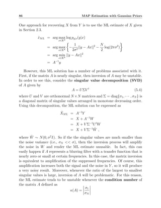

![88 MAP Estimation with Gaussian Priors
where µ(y) and R are given by
µ(y) = At
A + σ2
B
−1
At
y
R =
1
σ2
At
A + B
−1
,
and again c′
(y) is only a function of y. From the form of (5.7), we know that
px|y(x|y) must be conditionally Gaussian, with a conditional mean of µ(y)
and conditional variance of R. Therefore, the conditional density must have
the form
px|y(x|y) =
1
(2π)N/2
|R|−1/2
exp
−
1
2
(x − µ(y))t
R−1
(x − µ(y))
. (5.8)
Using the posterior distribution of (5.8), we can compute some typical
Bayesian estimators. Notice that the MMSE estimator is given by the con-
ditional mean,
x̂MMSE = E [X|Y = y] = µ(y) ,
and the MAP estimate is given by the conditional mode
x̂MAP = arg max
x∈RN
log pX|Y (x|y)
= arg min
x∈RN
1
2
(x − µ(y))t
R−1
(x − µ(y))
= µ(y) .
Notice that for this case, the MMSE and MAP estimates are the same. In
fact, this is always the case when all the random quantities in an estimation
problem are jointly Gaussian. However, we will find that the MMSE and
MAP are generally not the same when the distributions are non-Gaussian.
This will be important later since we will see that non-Gaussian distributions
are better models for image features such as edges.
5.2 Computing the MAP Estimate
So it seems that our problem is solved with the ubiquitous estimate
x̂ = At
A + σ2
B
−1
At
y . (5.9)](https://image.slidesharecdn.com/s6hfi7xht12wwcizuy0v-mbip-book-230123055619-8f2fce45/85/MBIP-book-pdf-98-320.jpg)

![90 MAP Estimation with Gaussian Priors
The general form of gradient descent iterations is given by
x(k+1)
= x(k)
− β∇f(x(k)
)
where x(k)
is the current image estimate, x(k+1)
is the updated image, and β
is a positive step size that determines how far one moves along the negative
gradiant direction. For the image restoration problem of (5.10), the gradient
of f(x) is given by
∇f(x) = −
1
σ2
At
(y − Ax) + Bx . (5.12)
So for this case, the gradient descent update equation is given by
x(k+1)
= x(k)
+ α[At
(y − Ax(k)
) − σ2
Bx(k)
] (5.13)
where α = β/σ2
is a scaled version of the step size. Rearranging terms, we
have the recursion
x(k+1)
= (I − α[At
A + σ2
B])x(k)
+ αAt
y . (5.14)
An important special case of (5.14) occurs when A represents a linear
space-invariant filter with 2-D impulse response as. When A represents a
space-invariant filter, then it has a Toeplitz-block-Toeplitz structure, and the
operation Ax is equivalent to the truncated 2-D convolution as ∗xs. Similarly,
multiplication by the transpose, At
y, is equivalent to 2-D convolution with the
space-reversed impulse response, a−s ∗ ys. In this case, the gradient descent
update equation of (5.13) has the form
x(k+1)
s = x(k)
s + α[a−s ∗ (ys − as ∗ x(k)
s ) − λ(δs − gs) ∗ x(k)
s ] , (5.15)
where gs is the non-causal predictor for the GMRF and λ = σ2
/σ2
x is a
measure of the noise-to-signal ratio. Here you can see that each iteration
of gradient descent is computed through the application of LSI filters; so as
long as the filter impulse response is spatially limited, the computation is not
excessive.
5.3.1 Convergence Analysis of Gradient Descent
Gradient descent is a simple algorithm, but it has a key disadvantage related
to the difficulty in selection of the step-size parameter. In order to better](https://image.slidesharecdn.com/s6hfi7xht12wwcizuy0v-mbip-book-230123055619-8f2fce45/85/MBIP-book-pdf-100-320.jpg)

![92 MAP Estimation with Gaussian Priors
To better understand why this is true, we can analyze the convergence
behavior of the gradient descent algorithm. Let us assume that the iteration
of (5.14) converges to the limit x(∞)
, then we can define the error in the
calculation of the MAP estimate to be ǫ(k)
= x(k)
− x(∞)
. In this case, we
know that taking the limit of (5.14) results in
x(∞)
= (I − α[At
A + σ2
B])x(∞)
+ αAt
y . (5.16)
Subtracting (5.14) and (5.16) results in
ǫ(k+1)
= I − α[At
A + σ2
B]
ǫ(k)
. (5.17)
We can further simplify the structure of (5.17) by using eigenvector analysis
of the matrix
H
△
= At
A + σ2
B .
Since H is symmetric, we know it can be diagonalized as H = EΛEt
where
columns of E are the orthonormal eigenvectors of H, and Λ = diag{h1, · · · , hN }
is a diagonal matrix containing the corresponding N eigenvalues of H. Notice
that the eigenvalues, hi, are all strictly positive because H is formed by the
sum of two positive-definite matrices. If we define the transformed error as
ǫ̃(k)
= Et
ǫ(k)
, then we may derive the following simple relationship for the
decay of the error in the gradient descent method.
ǫ̃(k)
= (I − αΛ)k
ǫ̃(0)
. (5.18)
Since Λ is diagonal, we can see that the ith
component of the error then
decays as
ǫ̃
(k)
i = (1 − αhi)k
ǫ̃
(0)
i . (5.19)
Equation (5.19) provides great insight into the convergence of gradient
descent to the MAP estimate. First, in order for convergence to be stable,
we must have that |1 − αhi| 1 for all i. Second, in order for convergence to
be rapid, we would like that 1 − αhi ≈ 0 for all i. As we will see, it is easy
to make convergence fast for one i, but it is generally not possible to make it
fast for all i.
A typical approach is to select α so that convergence is fast for the largest
eigenvalue, hmax = maxi{hi}. To do this we select α so that 1 − αhmax = 0,
which implies that
α =
1
hmax
.](https://image.slidesharecdn.com/s6hfi7xht12wwcizuy0v-mbip-book-230123055619-8f2fce45/85/MBIP-book-pdf-102-320.jpg)


![98 MAP Estimation with Gaussian Priors
converge faster at low spatial frequencies for problems that require deblurring
or deconvolution of an image. An alternative optimization approach with
faster convergence at high spatial frequencies is the iterative coordinate
descent (ICD) algorithm.1
ICD works by updating each pixel in sequence
while keeping the remaining pixels fixed. One full iteration of ICD then
consists of a sequence of single updates, were each pixel in x is updated
exactly once.
The ICD algorithm is most easily specified using the assignment notation
of a programming language. Using this notation, the value of the pixel xs is
updated using the rule
xs ← arg min
xs∈R
f(x)
while the remaining pixels xr for r 6= s remain unchanged. The result of an
ICD update of the pixel s can be compactly expressed as x + αεs where εs
is a vector that is 1 for element s, and 0 otherwise. Using this notation, we
have that
xs ← xs + arg min
α∈R
f(x + αεs) .
The ICD update can then be computed by solving the equation
0 =
∂f(x + αεs)
∂α
= [∇f(x + αεs)]t
εs ,
which results in
α =
(y − Ax)t
A∗,s − σ2
xt
B∗,s
||A∗,s||2 + σ2Bs,s
, (5.30)
where A∗,s and B∗,s denote the sth
column of A and B respectively. This then
results in the ICD update equation
xs ← xs +
(y − Ax)t
A∗,s − λ xs −
P
r∈∂s gs−rxr
||A∗,s||2 + λ
, (5.31)
where λ = σ2
σ2
x
is the effective noise-to-signal ratio.
Direct implementation of the ICD algorithm using (5.31) requires the eval-
uation of the term y − Ax with each pixel update. Typically, this requires
1
The Gauss-Seidel algorithm for solving differential equations works by updating each point in sequence
to meet the constraint of the differential equation. The Gauss-Seidel method is in many ways analogous to
ICD, and the techniques for analyzing the two algorithms are closely related.](https://image.slidesharecdn.com/s6hfi7xht12wwcizuy0v-mbip-book-230123055619-8f2fce45/85/MBIP-book-pdf-108-320.jpg)

![100 MAP Estimation with Gaussian Priors
−4 −2 0 2 4
0
0.5
1
1.5
2
2.5
3
3.5
4
Spectrum of Operator h(ω )
Frequency in Radians
Gain
−3 −2 −1 0 1 2 3
0
0.2
0.4
0.6
0.8
1
Spectrum of Operator P(ω) = U(ω )/( L(ω ) + h0
)
Frequency in Radians
Gain
−3 −2 −1 0 1 2 3
0
20
40
60
80
100
Number of ICD Iterations required for 99% Convergence
Frequency in Radians
Number
of
Iterations
(a) (b) (c)
Figure 5.6: Plots showing (a) the frequency response of h(ω), (b) the resulting func-
tion P(ω) = −L∗(ω)
L(ω)+h0
which determines the convergence rate of ICD, (c) the number
of iterations of ICD required for 99% convergence. Notice that ICD has more uni-
formly fast convergence across different frequencies as compared to gradient descent.
5.4.1 Convergence Analysis of Iterative Coordinate Descent
It is also possible to analyze the convergence of ICD, but the analysis is a bit
more tricky [67]. We first define the matrix
H
△
= At
A + σ2
B .
Using the gradient expression of (5.12), the scaled gradient of f(x) can then
be expressed as
σ2
∇f(x) = −At
y + Hx .
The objective of coordinate descent is to minimize the cost as a function of
the variable xs. So we enforce this condition by setting the sth
gradient term
to 0.
[∇f(x)]s =
−At
y + Hx
s
= 0
This can be more explicitly written as
−
X
r∈S
ar,syr +
X
r∈S
Hs,rxr = 0 . (5.33)
Now, let us assume that the ICD updates are performed in order. When
we update the pixel xs, the values of the previous pixels xr for r s will have
already been updated, and the values of xr for r s have yet to be updated.
This means that at the kth
iteration, the past pixels (i.e., r s) take on their
new value, xr = x
(k+1)
r , and the future pixels (i.e., r s) still retain their old](https://image.slidesharecdn.com/s6hfi7xht12wwcizuy0v-mbip-book-230123055619-8f2fce45/85/MBIP-book-pdf-110-320.jpg)


![5.6 Chapter Problems 105
5.6 Chapter Problems
1. Derive the expressions for µ(y) and R used in equation (5.7).
2. Consider a MAP estimation problem where the observations are given by
Y = AX + W where A ∈ RM×N
and X and W are independent jointly
Gaussian random vectors with distributions given by X ∼ N(0, B−1
),
W ∼ N(0, Λ−1
), where both B ∈ RN×N
and Λ ∈ RM×M
are symmetric
and positive-definite matrix.
a) Write an expression for the conditional density, py|x(y|x).
b) Write an expression for the prior density, px(x).
c) Write an expression for the MAP cost function, f(x), for this problem.
3. Consider the function
f(x) =
1
2
||y − Ax||2
Λ +
1
2
xt
Bx ,
where y ∈ RM
, x ∈ RN
, and B ∈ RN×N
is a symmetric positive semi-
definite matrix.
a) Calculate ∇f(x), the gradient of the cost function.
b) Calculate H(x), the Hessian matrix of the cost function given by
[H(x)]s,r =
∂2
f(x)
∂xs∂xr
c) Calculate the global minimum of the cost function.
4. Show that the update step for gradient descent with line search is given
by equations (5.27) and (5.29).
5. Show that the ICD update step is given by equation (5.30).
6. Let X ∈ RN
be an N pixel image that we would like to measure, and
let Y ∈ RN
be the noisy measurements given by
Y = AX + W
where A is an N × N nonsingular matrix, W is a vector of i.i.d. Gaus-
sian noise with W ∼ N(0, Λ−1
). Furthermore, in a Bayesian framework,](https://image.slidesharecdn.com/s6hfi7xht12wwcizuy0v-mbip-book-230123055619-8f2fce45/85/MBIP-book-pdf-115-320.jpg)


![114 Non-Gaussian MRF Models
6.2 Selection of Potential and Influence Functions
The question remains of how to select a potential function that best models
real images? One place to start is to look at the conditional distribution of a
pixel, xs, given its neighbors, x∂s. In particular, the most probable value of
xs given its neighbors is the solution to the optimization problem,
x̂s = arg max
xs∈R
log pxs|x∂s
(xs|x∂s)
= arg min
xs∈R
X
r∈∂s
bs,rρ(xs − xr) , (6.8)
which can be in turn computed as the solution to the equation
X
r∈∂s
bs,rρ′
(x̂s − xr) = 0 . (6.9)
Equation (6.8) has an interpretation of energy minimization where the terms
ρ(xs − xr) represent the potential energy associated with the two pixels xs
and xr. Alternatively, equation (6.9) has the interpretation of a force balance
equation where the terms ρ′
(x̂s − xr) represent the force that the pixel xr
exerts on the estimate x̂s.
This interpretation of ρ(xs − xr) as energy and ρ′
(xs − xr) as force serves
as a useful tool for the design and selection of these potential functions.
The function ρ′
(∆) is usually referred to as the influence function because
it determines how much influence a pixel xr has on the MAP estimate of a
pixel x̂s.
Figure 6.1 shows the potential and influence functions for two possible
choices of the potential function which we will refer to as the Gaussian
potential and Weak-spring potential [12, 11] functions.
Gaussian potential: ρ(∆) = |∆|2
Weak-spring potential: ρ(∆) = min
|∆|2
, T2
Notice that the weak-spring potential requires the choice of an additional
parameter T that we set to 1 for the plots. Along with each potential function,
we also show the associated influence function since this gives an indication of
the “force” resulting from neighboring pixels. Notice that with the Gaussian
prior, the influence of a pixel is linearly proportional to the value of ∆ =](https://image.slidesharecdn.com/s6hfi7xht12wwcizuy0v-mbip-book-230123055619-8f2fce45/85/MBIP-book-pdf-124-320.jpg)

![116 Non-Gaussian MRF Models
ture to the weak-spring potential. Each of these potential functions has the
property that ρ(∆) is a non-convex function of ∆. (Appendix A contains a
review of convexity including precise definitions and important properties.)
In fact, all non-convex potential functions have the property that their influ-
ence functions (i.e., derivatives) must sometimes decrease as ∆ increases.
Non-convex potential functions do a good job of precisely defining edges.
Intuitively, non-convex functions typically have a region |∆| Tc such that
ρ′
(∆) is strictly increasing (i.e., ρ(∆) is locally convex), and a region |∆| Tc
such that ρ′
(∆) is decreasing (i.e., ρ(∆) is locally concave). These two regions
clearly delineate between the “edge” and “non-edge” cases. However, in the
next section, we will also see that non-convex cost functions have limitations.
ρ(∆) Reference Potential Function Influence Function
min {|∆|2
, T}
Blake Zisserman [12,
11]
“Weak spring”
−2 0 2
0
1
2
3
Blake and Zisserman Potential
−2 0 2
−3
−2
−1
0
1
2
3
Blake and Zisserman Influence
∆2
T2+∆2 Geman McClure [35, 36]
−2 0 2
0
1
2
3
Geman and McClure Potential
−2 0 2
−3
−2
−1
0
1
2
3
Geman and McClure Influence
log (T2
+ ∆2
) Hebert Leahy [41]
−2 0 2
0
1
2
3
Hebert and Leahy Potential
−2 0 2
−3
−2
−1
0
1
2
3
Hebert and Leahy Influence
|∆|
T+|∆|
Geman Reynolds [31]
−2 0 2
0
1
2
3
Geman and Reynolds Potential
−2 0 2
−3
−2
−1
0
1
2
3
Geman and Reynolds Influence
Figure 6.2: List of the potential and influence functions for a variety of non-convex
potential functions plotted for T = 1.
While non-convex potential functions can preserve edges better than a
GMRF model, they also tend to generate discontinuous estimates at image
boundaries which are typically perceived as undesirable visual artifacts. For](https://image.slidesharecdn.com/s6hfi7xht12wwcizuy0v-mbip-book-230123055619-8f2fce45/85/MBIP-book-pdf-126-320.jpg)
![6.3 Convex Potential Functions 117
some applications, such as edge detection, this type of abrupt change at
edges can be desirable. However, in applications where the output needs to
be viewed as a physical image (i.e., photography, medical imaging, etc.), then
this type of very abrupt change can be undesirable.
Figures 6.3 illustrates how this discontinuous behavior can affect the result
of MAP estimation. Figure 6.3(a) shows two slightly different signals that
are used as input to a MAP cost function which uses the non-convex weak-
spring prior model. (See [15] for details of the experiment and model.) Notice
that only a slight change in the input, y, results in a discontinuous jump in
the MAP estimate shown in Figure 6.3(b). While this type of discontinuous
behavior can be desirable in applications such as edge detection, it is typically
not good when the result, x, is to be viewed as an image, or when it is
important to preserveF subtle details of continuous variation in the original
data.
-2
-1
0
1
2
3
4
5
6
0 5 10 15 20 25 30 35 40 45 50
Noisy Signals
signal #1
signal #2
Unstable Reconstructions
signal #1
signal #2
-2
-1
0
1
2
3
4
5
6
0 5 10 15 20 25 30 35 40 45 50
(a) (b)
Figure 6.3: Illustration of how the MAP estimate can actually be unstable in prac-
tice. Figure a) shows two slightly different signals that are used as input to a MAP
cost function incorporating non-convex potential functions. Notice that only a slight
change in the input, y, results in a discontinuous jump in the MAP estimate shown
in Figure b).
6.3 Convex Potential Functions
In this section, we introduce convex potential functions. Convexity is a very
important property of functions that is discussed in detail in Appendix A. A
potential function is convex if ∀a, b ∈ R and ∀λ ∈ R
ρ (λa + (1 − λ)) ≤ λρ(a) + (1 − λ)ρ(b) .](https://image.slidesharecdn.com/s6hfi7xht12wwcizuy0v-mbip-book-230123055619-8f2fce45/85/MBIP-book-pdf-127-320.jpg)
![118 Non-Gaussian MRF Models
Convex potential functions have two major advantages when the data term
is also convex. First, they result in continuous or stable MAP estimates, so
the resulting images tend to have fewer undesirable artifacts. And second,
the resulting optimization problem for MAP estimation is also convex, so it
is typically possible to compute the global maximum of the posterior density
in tractable time.
ρ(∆) Reference Potential Function Influence Function
∆2
2
Gaussian MRF
“Quadratic”
−2 0 2
0
1
2
3
Gaussian (L2
) Potential
−2 0 2
−3
−2
−1
0
1
2
3
Gaussian (L
2
) Influence
|∆| Besag[10]
“Total Variation”
−2 0 2
0
1
2
3
Total Variation (L
1
) Potential
−2 0 2
−3
−2
−1
0
1
2
3
Total Variation (L
1
) Influence
|∆|p
p
Bouman Sauer[15]
“Generalized Gaussian
MRF”
−2 0 2
0
1
2
3
Generalized Gaussian Potential
−2 0 2
−3
−2
−1
0
1
2
3
Generalized Gaussian Influence
(∆2
2 for |∆|T
T|∆|− T2
2 for |∆|≥T
Stevenson Delp[73]
“Huber function”
−2 0 2
0
1
2
3
Huber Function Potential
−2 0 2
−3
−2
−1
0
1
2
3
Huber Function Influence
T2
log cosh
|∆|
T
Green [37]
−2 0 2
0
1
2
3
log cosh Potential
−2 0 2
−3
−2
−1
0
1
2
3
log cosh Influence
|∆|p
p
|∆/T|q−p
1 + |∆/T|q−p
Thibault, Sauer,
Bouman, Hsieh[74]
“Q-Generalized GMRF”
−2 0 2
0
1
2
3
Q−Generalized Gaussian Potential
−2 0 2
−3
−2
−1
0
1
2
3
Q−Generalized Gaussian Influence
Figure 6.4: List of the potential and influence functions for a variety of convex po-
tential functions for T = 1 and shape parameters p = 1.2 and q = 2.](https://image.slidesharecdn.com/s6hfi7xht12wwcizuy0v-mbip-book-230123055619-8f2fce45/85/MBIP-book-pdf-128-320.jpg)
![6.3 Convex Potential Functions 119
Over the years, a wide variety of convex potential functions have been
proposed with a correspondingly wide range of practical and theoretical ad-
vantages and disadvantages to consider. Figure 6.4 shows a representative
subset of these functions, although there are many more.
Of course, the simplest choice of potential function is the quadratic, ρ(∆) =
∆2
, which results in the Gaussian MRF model that was the subject of Chap-
ter 4. While this model has the advantage of being the most analytically
tractable, its primary disadvantage is that it does not accurately characterize
the sharp discontinuities that typically occur in images and other real signals.
One of the earliest and most interesting alternative potential functions is
the absolute value function initially proposed by Besag [10], which is some-
times referred to as a L1 norm regularizer. In this case, the potential function
is given by
ρ(∆) = |∆| , (6.10)
with associated influence function
ρ′
(∆) = sign(∆) . (6.11)
This potential function has the advantages that it is convex; it does not grow
as quickly as a quadratic function, so it is edge preserving; and it does not
require the choice of a specific T parameter that determines the value of ∆
that will likely occur across edges.
The absolute value potential function represents a special case because it
is convex, but not strictly convex; and because it has a discontinuous second
derivative at 0. This results in many very unique properties to the MAP
estimate. For example, because the MAP cost function is not continuously
differentiable, gradient based algorithms such as gradient descent, conjugate
gradient and ICD are generally not convergent when used with the abso-
lute value potential function, and more complex optimization algorithms are
required that often are not guaranteed to achieve the global minimum [66].
We should note that the absolute value potential function is very closely
related to the total variation regularization of [65] in which image esti-
mates are regularized using the integral of the gradient magnitude. The total
variation norm is defined for continuous functions on R2
by
TV (x) =
Z
R2
|∇x(r)|dr .](https://image.slidesharecdn.com/s6hfi7xht12wwcizuy0v-mbip-book-230123055619-8f2fce45/85/MBIP-book-pdf-129-320.jpg)
![120 Non-Gaussian MRF Models
But of course in applications, it is necessary to discretely sample the function
x(r). So the TV norm can be discretely approximated, using a rectangular
sampling lattice, by either the isotropic total variation given by
TV (x) =
X
i,j
q
(xi+1,j − xi,j)2
+ (xi,j+1 − xi,j)2
, (6.12)
or the anisotropic total variation given by
TV (x) =
X
i,j
|xi+1,j − xi,j| + |xi,j+1 − xi,j| . (6.13)
Notice that the anisotropic total variation of (6.13) is a special case of the
pair-wise Gibbs distribution with the absolute value potential function. How-
ever, as the name implies, the anisotropic total variation of (6.13) does not
accurately approximate the total variation for all orientations of the gradient.
Nonetheless, its simplified form sometimes has computational advantages.
Figure 6.5 illustrates what typically happens when absolute value poten-
tials are used. Notice that the minimum of the cost function typically falls
along these edges of discontinuity. Since the edges of discontinuity occur with
|xr − xs| = 0 or equivalently, xr = xs, the MAP estimate tends to contain
groups of neighboring pixels that are of equal value. This means that the
absolute value potential tends to produce large flat regions with sharp transi-
tions. In some cases, this may be good, but in other cases, these flat regions
can appear artificial and are often described as “waxy” by naive observers.
In some applications, this tendency of the absolute value potential function
or L1 norm log prior model to drive values to zero can be quite useful. For ex-
ample, the least absolute shrinkage and selection operator (LASSO)
uses this property of the L1 norm to drive model parameter values to 0,
thereby reducing model order [75].
However, in other applications, the L1 norm’s tendency to zero out reg-
ularized quantities can result in image artifacts; so in these applications, a
less severe regularizing potential function is needed. There are two basic ap-
proaches to addressing this limitation of absolute value prior models. One
approach is to generalize the L1 norm to an Lp norm, and a second approach
is to “round out” the bottom of the L1 norm by making it quadratic for
|∆| 1.](https://image.slidesharecdn.com/s6hfi7xht12wwcizuy0v-mbip-book-230123055619-8f2fce45/85/MBIP-book-pdf-130-320.jpg)
![6.3 Convex Potential Functions 121
xr
f(xs, xr; y)
xs
xs = xr
x̂MAP = arg min
xs,xr
f(xs, xr; y)
Figure 6.5: Figure showing a typical MAP cost function resulting from the use of a
absolute value potential function (i.e., total variation regularization). Notice that the
cost function is convex, but that it is not continuously differentiable, so that the min-
imum of the cost function typically occurs at a point of discontinuity corresponding
to xs = xr where r ∈ ∂s.
An example of the first approach is the potential function used for the
Generalized Gaussian MRF (GGMRF) [15]. In this case, the potential
function is given by
ρ(∆) =
|∆|p
p
, (6.14)
with associated influence function
ρ′
(∆) = |∆|p−1
sign(∆) . (6.15)
For p 1 this potential function is strictly convex and continuously differ-
entiable; so gradient based algorithms can achieve a global minimum of the
cost function. In addition, these potential functions have the advantage that,
as with the case of the absolute value potential, there is no longer an explicit
value of T to choose, but there is instead a general shape parameter p. In
practice, p is often chosen to be in the range of 1.1 to 1.2.
Another approach to generalizing the absolute value potential is to round
out the point of the function by using a local quadratic near ∆ = 0. Perhaps
the best example of this approach is the Huber function [73]. This potential
function is given by
ρ(∆) =
(
∆2
2 for |∆| T
T|∆|−T2
2 for |∆| ≥ T ,
(6.16)](https://image.slidesharecdn.com/s6hfi7xht12wwcizuy0v-mbip-book-230123055619-8f2fce45/85/MBIP-book-pdf-131-320.jpg)
![122 Non-Gaussian MRF Models
with associated influence function
ρ′
(∆) = clip{∆, [−T, T]} , (6.17)
where the function clip{x, [a, b]} simply clips the value x to the interval [a, b].
The Huber function has the advantage that near ∆ = 0 it maintains many
of the properties of the GMRF. This can be very important because the
images generated with Huber function potentials tend to better maintain
low-contrast details, and they also result in MAP cost functions that are
more amenable to optimization. However, the Huber function does have
some disadvantages. First, it again requires the choice of a threshold T.
Second, for values of |∆| T, the function is not strictly convex, so the
global minimum of the MAP cost function may not be unique; and finally,
the function does not have a continuous second derivative at |∆| = T. This
last disadvantage is easily addressed by a wide variety of alternative potential
functions which are approximately quadratic at ∆ = 0, and approximately
linear as |∆| → ∞. One such example is the function
ρ(∆) = T2
log cosh
|∆|
T
, (6.18)
with associated influence function
ρ′
(∆) = T tanh
|∆|
T
, (6.19)
where again the constant T is introduced to control the placement of the
transition from quadratic to linear behavior [37].
Finally, the Q-Generalized GMRF (QGGMRF) is a generalization of
the GGMRF potential function that allows for parameters to control both
the low-contrast character of the function when ∆ ≈ 0, and the high-contrast
character as |∆| → ∞ [74]. The QGGMRF potential function is given by
ρ(∆) =
|∆|p
p
∆
T
q−p
1 + ∆
T
q−p
!
(6.20)
and its associated influence function is given by
ρ′
(∆) = |∆|p−1
∆
T
q−p
q
p + ∆
T
q−p
1 + ∆
T
q−p
2 sign(∆) (6.21)](https://image.slidesharecdn.com/s6hfi7xht12wwcizuy0v-mbip-book-230123055619-8f2fce45/85/MBIP-book-pdf-132-320.jpg)
![6.4 Scaling Parameters for Non-Gaussian MRFs 123
where p and q are chosen so that 1 ≤ p q in order to ensure that the
function is convex.4
Along high contrast edges, when |∆| T, the shape
of the QGGMRF is approximately the same as the GGMRF with ρ(∆) ≈
|∆|p
p . However, in low-contrast regions when |∆| T, then the potential
function is approximately given by ρ(∆) ≈ |∆|q
pTq−p . In a typical application,
one might choose q = 2 and 1 ≤ p q. In this case, the potential function
is quadratic near ∆ = 0 and is ensured to have a continuous first and second
derivative. Notice that this is not the case for the function |∆|p
, which has an
unbounded second derivative near ∆ = 0 when 1 ≤ p 2. Later we will see
that a continuous second derivative is a valuable property in optimization,
particularly when using the majorization techniques of Chapter 8.
6.4 Scaling Parameters for Non-Gaussian MRFs
In practical problems, it is almost always necessary to scale the range of values
for a MRF model. So for example, if an MRF, X, represent a conventional
raster image, then the values, Xs, should fall in a range from 0 to 255.
However, if X is being used to represent ocean depth in meters, then a range
of 0 to 11,000 might be more appropriate. So for each physical phenomena,
we must be able to scale the typical range of values in a MRF model, without
necessarily changing the basic characteristics of the model.
To do this, we can introduce a scaling parameter, σx, to the pair-wise Gibbs
distribution of equation (6.5). We do this by directly scaling the values inside
the potential functions of the Gibbs distribution.
p(x|σx) =
1
z
exp
−
X
{s,r}∈P
bs,rρ
xs − xr
σx
Using this convention, notice that if X has distribution p(x|σx), then X̃ =
X/σx must have a distribution given by p(x|σx = 1).
Even though parameter estimation for MRFs is known to be a classically
difficult problem, estimation of the scale parameter, σx, is more tractable
then one might imagine. This is because the partition function, z, turns
4
Our definition of the QGGMRF swaps the roles for the variables q and p relative to the form used in
[74].](https://image.slidesharecdn.com/s6hfi7xht12wwcizuy0v-mbip-book-230123055619-8f2fce45/85/MBIP-book-pdf-133-320.jpg)

![6.4 Scaling Parameters for Non-Gaussian MRFs 125
Name Potential Function ρ(∆) Influence Function ρ′(∆)
Quadratic
∆2
2σ2
x
∆
σ2
x
Total
Variation
|∆|
σx
sign(∆)
σx
Huber
∆2
2σ2
x
for |∆|Tσx
T ∆
σx
− T2
2 for |∆|≥Tσx
1
σ2
x
clip{∆, [−Tσx, Tσx]}
log cosh T2
log cosh
∆
Tσx
T
σx
tanh
∆
Tσx
GGMRF
|∆|p
pσp
x
|∆|p−1
σp
x
sign(∆)
QGGMRF
|∆|p
pσp
x
∆
Tσx
q−p
1 + ∆
Tσx
q−p
|∆|p−1
σp
x
∆
Tσx
q−p
q
p + ∆
Tσx
q−p
1 + ∆
Tσx
q−p
2 sign(∆)
Table 6.1: Analytical expressions for a number of convex potential functions and
their associated influence function. Each potential function is parameterized by a
scale parameter, σx, and a threshold parameter, T. The scale parameter changes the
range of values in X, and the threshold parameter determines the point of transition
in the potential functions.
Notice, that the very simple form of equation (6.23) is reminiscent of the
expression for the variance of a Gaussian random variable, except that the
sum is over all cliques and the differences are raised to the power p rather
than simply squared.
The setting of the single parameter σx can be a major practical concern
when using p(x) as a prior model in, say, MAP estimation. If σx is too large,
then the image will be “under regularized” or in other words, it will over-fit
the measured data and have too much noisy variation. Alternatively, if σx is
too small, the image will be “over regularized” and important detail may be
removed due to over smoothing.
For notational simplicity, we can just include this parameter, σx, in the
definition of the potential function. So for example, in the quadratic case the
potential function becomes
ρ(∆) =
1
2
∆
σx
2
=
∆2
2σ2
x](https://image.slidesharecdn.com/s6hfi7xht12wwcizuy0v-mbip-book-230123055619-8f2fce45/85/MBIP-book-pdf-135-320.jpg)


![130 MAP Estimation with Non-Gaussian Priors
properties that restrict the image to a convex set Ω ⊂ RN
. For example, in
many physical problems we know that the solution must by non-negative, so
we would like to enforce a positivity constraint when solving the problem.
To do this, we first define the set R+
= {x ∈ R : x ≥ 0}, and then the convex
set is given by
Ω = R+N
=
x ∈ RN
: xi ≥ 0 for all i . (7.1)
Using this framework, the MAP estimate of X given Y is given by
x̂ = arg min
x∈Ω
f(x; y) , (7.2)
where we will refer to the function f(x; y) as the MAP cost function given
by
f(x; y) = − log py|x(y|x) − log p(x) . (7.3)
So the three key steps required for MAP estimation are:
1. Select the forward model py|x(y|x);
2. Select the prior model p(x);
3. Minimize the cost function.
In principle, only steps 1 and 2 determine the quality of the MAP estimate,
and the choice of optimization procedure only affects the computation re-
quired to compute the estimate. However, in practice if the optimization
method does not achieve the exact global minimum of the MAP cost func-
tion (which is typically the case), then step 3 will also have some impact on
the quality of the solution.
Convexity of the MAP cost function, f(x; y), as a function of x will be a
very powerful concept in understanding the existence, uniqueness, and stabil-
ity of the MAP estimate.1
Appendix A provides a review of convex functions
and sets, and it also provides some basic results on how convexity can be
used to ensure existence and uniqueness of minima in general, and the MAP
estimate in particular. Loosely speaking, the key results are that, for a con-
vex function, any local minimum must also be a global minimum; and for a
strictly convex function, any global minimum must be unique.
1
Existence, uniqueness, and stability are the three properties of a well-posed inverse as defined by
Tikhonov[76].](https://image.slidesharecdn.com/s6hfi7xht12wwcizuy0v-mbip-book-230123055619-8f2fce45/85/MBIP-book-pdf-140-320.jpg)

![132 MAP Estimation with Non-Gaussian Priors
the data y. The following theorem makes this statement more precise [15].
Theorem 7.1.1. Stability/Continuity of MAP Estimates
Let the MAP cost function, f(x; y), be a continuous function of (x, y) ∈
Ω × RM
; and for all y ∈ RM
, let f(·, y) be a strictly convex function of x ∈ Ω
with a local minimum. Then the MAP estimate is a unique and continuous
(i.e., stable) function of the data y.
This raises the question of what conditions will ensure convexity of the
MAP cost function? In order to provide a practical answer to this question,
we will consider a slightly more general example than the one considered in
Chapter 5. Let us assume that Y ∈ RM
has the form
Y = AX + W , (7.4)
where W ∈ RM
is assumed to be independent zero-mean additive Gaussian
noise with distribution N(0, Λ−1
), X ∈ RN
, and A is an M × N matrix.
Typically, the inverse covariance Λ is diagonal because the noise for each
scalar observation is independent; however, this is not absolutely necessary
for the formulation of our problem. In addition, it may happen that M N,
M N, or M = N depending on the specific experimental scenario.
Given this framework, the likelihood of the observations, Y , given the
unknown, X, has a form similar to equation (5.3).
py|x(y|x) =
1
(2π)M/2
|Λ|1/2
exp
−
1
2
||y − Ax||2
Λ
(7.5)
In addition, we assume that X is an MRF, so that the prior is given by a
pair-wise Gibbs distribution similar to that of equation (6.5),
p(x) =
1
z
exp
−
X
{s,r}∈P
bs,rρ(xs − xr)
, (7.6)
where in this case the potential function ρ(∆) includes the scaling constant
σx as shown in Table 6.1 of Section 6.4. Putting the forward and prior models
into equation (7.3), we get the MAP cost function of
f(x; y) =
1
2
||y − Ax||2
Λ +
X
{s,r}∈P
bs,rρ(xs − xr) . (7.7)](https://image.slidesharecdn.com/s6hfi7xht12wwcizuy0v-mbip-book-230123055619-8f2fce45/85/MBIP-book-pdf-142-320.jpg)


![7.2 General Approaches to Optimization 137
In fact, the ICD algorithm we have studied is guaranteed to converge to the
global minimum under some fairly general conditions. The following theorem
states this result more precisely.
Theorem 7.2.1. ICD Convergence
Let f : Ω → R be a strictly convex and continuously differentiable function on
the convex set Ω ⊂ RN
. Then the ICD iterations of equation (7.10) converge
to the global minimum of f.
Proof. See for example Proposition 3.9 page 219 of [6].
However, while this result appears to be strong, the limitation to con-
tinuously differentiable functions is a practical restriction. If the function
is convex but not differentiable, then the ICD algorithm can routinely fail
to converge. For example, when using the total variation regularization of
Section 6.3, the MAP cost function is not continuously differentiable, so the
ICD algorithm will typically stall before reaching the global minimum. The
Problems 7 and 5 at the end of this chapter present two examples of the ap-
plication of ICD to functions that are not continuously differentiable. In the
first problem, ICD can be shown to converge to the global minimum, while
in the second problem it stalls.
One important advantage of ICD is that positivity is easily enforced by
simply restricting each update to take on a non-negative value. In this case,
the ICD optimization procedure is given by
xs ← xs + arg min
α≥−xs
f(x + αεs) ,
where εs is a vector which is 1 at its sth
coordinate and zero elsewhere.
Figure 7.3 shows a pseudo-code specification of the general ICD optimization
algorithm with positivity constraints.
If the function f(x) is continuously differentiable and convex, then the
solution to the optimization problem with positivity constraints can be ex-
pressed using the KKT conditions. In this case, the KKT conditions reduce](https://image.slidesharecdn.com/s6hfi7xht12wwcizuy0v-mbip-book-230123055619-8f2fce45/85/MBIP-book-pdf-147-320.jpg)

![7.3 Optimization of the MAP Cost Function 139
the log likelihood term has a quadratic form, equation (7.12) can be more
compactly expressed as a simple quadratic function of the scalar value α.
We can do this by simply computing the first two terms of the Taylor series
expansion, which in this case, will be an exact representation of the true log
likelihood. This results in the following simpler expression for the MAP cost
function
f(x + αd) = c + θ1α +
1
2
θ2α2
+
X
{s,r}∈P
bs,rρ(∆xs,r + α∆ds,r) (7.13)
where
θ1 = −et
ΛAd (7.14)
θ2 = dt
At
ΛAd , (7.15)
where e = y − Ax. So our objective is then to minimize this function over α,
and then to use this minimized value to update x. The optimal value of α is
then given by
α∗
= arg min
α∈[a,b]
f(x + αd) (7.16)
= arg min
α∈[a,b]
θ1α +
1
2
θ2α2
+
X
{s,r}∈P
bs,rρ(∆xs,r + α∆ds,r)
(7.17)
where [a, b] is the interval over which α can vary. For example, in gradient
descent [a, b] = [0, ∞]. However, in practice it is usually possible to find
tighter limits which result in a bounded interval. Once the value of α∗
is
computed, then the value of x is updated,
x ← x + α∗
d ,
and the entire optimization procedure is repeated until sufficient convergence
is achieved.
The following example considers the special case of ICD optimization and
derives an efficient algorithm for computing the required updates.
Example 7.1. In order to illustrate the concept of non-quadratic line search,
consider the example of ICD updates with a non-quadratic log prior model.](https://image.slidesharecdn.com/s6hfi7xht12wwcizuy0v-mbip-book-230123055619-8f2fce45/85/MBIP-book-pdf-149-320.jpg)


![142 MAP Estimation with Non-Gaussian Priors
Half Interval Line-Search Algorithm:
Initialize a and b so that g(a) 0 and g(b) 0.
For k = 1 to K {
c ← (a + b)/2
If g(c) ≤ 0, then a ← c
If g(c) 0, then b ← c
}
α∗
= −g(a)
g(b)−g(a)
(b − a) + a
Figure 7.5: This figure provides a pseudocode specification of half-interval line search.
The algorithm requires an initial specification of the search interval, [a, b], and then
it iteratively halves the interval to reduce the uncertainly of the solutions.
then c is taken as the new right hand end of the interval. After K iterations,
the algorithm is guaranteed to have achieved an accuracy of at least b−a
2K .
Notice that the last step performs an interpolation of the function in order
to estimate the location of the root. If the function is smooth, then this step
can greatly improve the rooting accuracy.
However, half interval search has a number of disadvantages. First, it
requires that a finite interval, [a, b], for the solution be known in advance.
There are a number of practical approaches to solving this problem. One
approach is to first check the values of g(a) and g(b). If both g(a) 0 and
g(b) 0, then a ← b can be taken as the new left-hand value, since it is
the better of the two solutions, and the value of b can be increased. This
process can then be repeated until g(b) 0. A similar approach can be taken
if g(a) 0 and g(b) 0. In this case, b ← a and a is decreased.
Perhaps a more serious disadvantage of half-interval search is that it re-
quires repeated evaluation of the function g(α). Typically, evaluation of g(α)
requires significant computation, so this may represent an unacceptable com-
putational overhead. This overhead can be reduced by the judicious design
of a line search algorithm which converges in a small number of iterations.
Furthermore, it is important that with each iteration the value of the cost
function, f(x + αd), is monotonically decreased from its starting value, f(x).
This ensures that, even if the iterations are terminated early, the cost function
will still be reduced. The following chapter presents such an approach.](https://image.slidesharecdn.com/s6hfi7xht12wwcizuy0v-mbip-book-230123055619-8f2fce45/85/MBIP-book-pdf-152-320.jpg)


![Chapter 8
Surrogate Functions and Majorization
As non-quadratic optimization has grown in importance, a very powerful set
of methods have emerged known as majorization techniques, which allow
non-quadratic optimization problems to be converted into iterative quadratic
optimization. These methods go by a variety of names, but they all share a
similar framework.1
The idea behind majorization techniques is to approxi-
mate the true function being minimized by a much simpler function known
as a surrogate or substitute function.
In this chapter, we introduce the concepts of surrogate functions and ma-
jorization as powerful tools for efficiently computing the solution to the non-
quadratic optimization problems resulting from MAP estimation with non-
Gaussian models. We will see that surrogate functions can be very effective
in a broad range of optimization problems because they allow for dramatic
simplification of problems without sacrificing accuracy or convergence speed.
Later in Chapter 12, we will also see that surrogate functions play a central
role in understanding the EM algorithm.
1
Over the years, roughly equivalent methods have been “rediscovered” for differing purposes, and many
of these rediscoveries have resulted in new names for the method. One of the earliest references is the
majorant technique of Kantorovich in [45] as a method for insuring the convergence of Newton iterations.
Of course, the EM algorithm first introduced in its general form in [3, 2] implicitly uses this method for
the iterative computation of the ML estimate. Ortega and Rheinboldt later discussed the method in the
context of line search and referred to it as the “majorization principal” [56]. In [43], Huber used the concept
of “global” curvature to minimize 1-D functions resulting from robust estimation procedures. This same
concept was called “half-quadratic optimization” and applied to the problem of regularization or MAP
estimation using non-quadratic priors by Geman in [32]. And, De Pierro introduced the concept to the
image reconstruction community for the purposes of parallel optimization in tomographic reconstruction in
[60]. The terms surrogate function [26] and substitute function [83] were later used to describe a technique
for the parallelization of coordinate descent optimization in tomographic reconstruction.](https://image.slidesharecdn.com/s6hfi7xht12wwcizuy0v-mbip-book-230123055619-8f2fce45/85/MBIP-book-pdf-157-320.jpg)


![156 Surrogate Functions and Majorization
Name ρ(∆)
ρ′(∆′)
2∆′
ρ′′(0)
2
Quadratic
∆2
2σ2
x
1
2σ2
x
1
2σ2
x
Total
Variation
|∆|
σx
1
2σx|∆′|
∞
Huber
∆2
2σ2
x
for |∆|Tσx
T ∆
σx
− T2
2 for |∆|≥Tσx
clip{∆′, [−Tσx, Tσx]}
2σ2
x∆′
1
2σ2
x
log cosh T2
log cosh
∆
Tσx
T tanh
∆′
Tσx
2σx∆′
1
2σ2
x
GGMRF
|∆|p
pσp
x
|∆′|p−2
2σp
x
∞ for 1 ≤ p 2
QGGMRF
(p ≤ q)
|∆|p
pσp
x
∆
Tσx
q−p
1 + ∆
Tσx
q−p
|∆′|p−2
2σp
x
∆′
Tσx
q−p
q
p + ∆′
Tσx
q−p
1 + ∆′
Tσx
q−p
2
1
pσ2
xT2−p
for q = 2
Table 8.1: Analytical expressions for the coefficients used in the symmetric bound of
equation (8.17).
practice, this is a common property for practical potential functions since
it means that the influence of pixels will decrease as the difference between
pixels increases.
Table 8.1 lists out the analytical expressions for the terms of equation (8.17)
for each of the potential functions we have discussed. Notice that some of
the expressions for ρ′′
(0)/2 are unbounded. For example, this is the case for
the total variation potential function because its second derivative becomes
unbounded at zero. This represents a real practical problem when using sur-
rogate functions. In fact, a major advantage of the Huber and QGGMRF
potentials is that they have bounded second derivatives at zero; so both these
potential functions are compatible with surrogate optimization methods. In
Chapter 9 we will address this problem by introducing new algorithms that
can be used when computing the MAP estimate with potential functions such
as the total variation prior.
Substituting the symmetric bound surrogate function of (8.17) into equa-](https://image.slidesharecdn.com/s6hfi7xht12wwcizuy0v-mbip-book-230123055619-8f2fce45/85/MBIP-book-pdf-166-320.jpg)
![8.3 Minimizing the MAP Cost Function 157
tion (8.12) results in the following MAP surrogate cost function,
Q(x; x′
) =
1
2
||y − Ax||2
Λ +
X
{s,r}∈P
bs,rρ′
(x′
s − x′
r)
2(x′
s − x′
r)
(xs − xr)2
, (8.18)
where for simplicity we assume that x′
s −x′
r 6= 0. Below is an example of how
this method can be applied for a particular choice of potential function.
Name Surrogate Function Coefficient b̃s,r of Equation (8.19)
General b̃s,r ← bs,r
ρ′(x′
s − x′
r)
2(x′
s − x′
r)
Quadratic b̃s,r ← bs,r
1
2σ2
x
Total
Variation
b̃s,r ← bs,r
1
2σx|x′
s − x′
r|
Huber b̃s,r ← bs,r
clip{x′
s − x′
r, [−Tσx, Tσx]}
2σ2
x(x′
s − x′
r)
log cosh b̃s,r ← bs,r
T tanh
x′
s−x′
r
Tσx
2σx(x′
s − x′
r)
GGMRF b̃s,r ← bs,r
|x′
s − x′
r|p−2
2σp
x
QGGMRF b̃s,r ← bs,r
|x′
s − x′
r|p−2
2σp
x
x′
s−x′
r
Tσx
q−p
q
p + x′
s−x′
r
Tσx
q−p
1 + x′
s−x′
r
Tσx
q−p
2
Table 8.2: Analytical expressions for the coefficient b̃s,r required for computing the
surrogate function using the symmetric bound method. Each expression corresponds
to a potential function given in Table 6.1 of Section 6.4.
An alternative way to think about the surrogate function approach is that
with each iteration, we recompute the local coefficients, bs,r. Using this point
of view, we can express the surrogate MAP cost function as
b̃s,r ← bs,r
ρ′
(x′
s − x′
r)
2(x′
s − x′
r)
(8.19)
Q(x; x′
) =
1
2
||y − Ax||2
Λ +
X
{s,r}∈P
b̃s,r (xs − xr)2
, (8.20)](https://image.slidesharecdn.com/s6hfi7xht12wwcizuy0v-mbip-book-230123055619-8f2fce45/85/MBIP-book-pdf-167-320.jpg)
![158 Surrogate Functions and Majorization
where the coefficients, b̃s,r, are the modified coefficients that are updated with
each iteration of an optimization algorithm.
So in practice, in order to implement a particular potential function one
simply computes the values of b̃s,r corresponding to their desired choice of po-
tential function. Table 8.2 lists out the specific formulas for the coefficients,
b̃s,r, for each of the potential functions we have considered in Table 6.1. While
the formulas might seem a bit messy, the approach is straightforward. One
simply calculates the value of b̃s,r corresponding to the desired potential func-
tion, and then minimizes the quadratic cost function of equation (8.20) with
respect to x.
Example 8.1. In this example, we find the symmetric bound surrogate func-
tion for the Huber potential listed in Table 6.1 of Section 6.4. In this case,
the potential function is given by
ρ(∆) =
∆2
2σ2
x
for |∆| Tσx
T ∆
σx
−T2
2 for |∆| ≥ Tσx
,
and its associated influence function is given by
ρ′
(∆) =
1
σ2
x
clip{∆, [−Tσx, Tσx]} ,
where the function clip{x, [a, b]} clips the value x to the interval [a, b]. For
the symmetric bound, the surrogate function of equation (8.17) is given by
ρ(∆; ∆′
) =
clip{∆′
, [−Tσx, Tσx]}
2σ2
x∆′
∆2
. (8.21)
Notice that the result of equation (8.21) corresponds to the entry labeled
“Huber” in Table 8.2. So in practice, we could have skipped this analysis,
and referred directly to the Table to find the update for the b̃s,r terms given
by
b̃s,r ←
bs,r
clip{x′
s − x′
r, [−Tσx, Tσx]}
2σ2
x(x′
s − x′
r)
for x′
s 6= x′
r
bs,r
2σ2
x
for x′
s = x′
r
,](https://image.slidesharecdn.com/s6hfi7xht12wwcizuy0v-mbip-book-230123055619-8f2fce45/85/MBIP-book-pdf-168-320.jpg)
![8.4 Application to Line Search 159
where we explicitly add the case when x′
s = x′
r. From this, the symmetric
bound MAP surrogate cost function is given by
Q(x; x′
) =
1
2
||y − Ax||2
Λ +
X
{s,r}∈P
b̃s,r (xs − xr)2
. (8.22)
The MAP estimate can then be computed though repeated minimization of
(8.22). Since the function is now a quadratic function of x, a wide variety of
optimization algorithms can be used for this purpose.
8.4 Application to Line Search
In order to better understand how surrogate functions can be used, let us
next consider its application to the important problem of line-search opti-
mization discussed in Section 7.2. In this case, our objective is to solve the
1-D minimization problem
α∗
= arg min
α∈[a,b]
f(x + αd) ,
where x ∈ RN
is the current value of the solution, d ∈ RN
is the update
direction, α is the unknown update step size, and [a, b] is a search interval
that includes 0.
Using a surrogate function in place of f(x), we compute the modified line
search
α∗
= arg min
α∈[a,b]
Q(x + αd; x) ,
where we assume that α ∈ [a, b]. Now since the surrogate MAP cost function
of equation (8.22) is a quadratic function of x, we can use the same trick and
express the line search function as a quadratic function of α,
Q(x + αd; x) = c + θ1α +
1
2
θ2α2
,
where it can be shown that (See problem 4)
θ1 = −(y − Ax)t
ΛAd +
X
{s,r}∈P
2b̃s,r (xs − xr) (ds − dr) (8.23)
θ2 = dt
At
ΛAd +
X
{s,r}∈P
2b̃s,r (ds − dr)2
. (8.24)](https://image.slidesharecdn.com/s6hfi7xht12wwcizuy0v-mbip-book-230123055619-8f2fce45/85/MBIP-book-pdf-169-320.jpg)
![160 Surrogate Functions and Majorization
General MAP Optimization using Majorization of Prior:
Initialize x
For K iterations {
{d, a, b} ← SelectSearchDirectionAndInterval(x)
b̃s,r ←
bs,rρ′
(xs − xr)
2(xs − xr)
θ1 ← −(y − Ax)t
ΛAd +
X
{s,r}∈P
2b̃s,r (xs − xr) (ds − dr)
θ2 ← dt
At
ΛAd +
X
{s,r}∈P
2b̃s,r (ds − dr)2
α∗
← clip
−θ1
θ2
, [a, b]
x ← x + dα∗
}
Figure 8.4: Pseudocode for the implementation of a general MAP optimization pro-
cedure that uses majorization of the prior term. Each line search is approximately
solved by replacing the true prior term with a surrogate function.
In this case, the line search solution has the very simple form of
α∗
= clip
−θ1
θ2
, [a, b]
.
Figure 8.4 provides a pseudocode specification of a generic optimization
algorithm which uses this majorization approach in the line search step. The
search direction may vary based on the specific choice of optimization al-
gorithm, but the computation of the line search always follows the same
procedure. Notice that the resulting value of α∗
guarantees that
f(x + α∗
d) − f(x) ≤ Q(x + α∗
d; x) − Q(x; x) ≤ 0 ,
so we know that the true cost function decreases with each iteration of this
algorithm. The advantage of this modified line search is that the 1-D opti-
mization can be computed very efficiently in one step. This is in contrast
to the many iterations that may be required of the half-interval search of
Section 7.2.
Example 8.2. In this example, we derive the explicit expressions for ICD
updates using a symmetric surrogate function. For the ICD algorithm, the](https://image.slidesharecdn.com/s6hfi7xht12wwcizuy0v-mbip-book-230123055619-8f2fce45/85/MBIP-book-pdf-170-320.jpg)


![9.2 The Lagrangian and Dual Function 171
In this case, equation (9.6) represents a convex optimization problem. Of
course, this is not the most general form of the constrained optimization
problem. For example, the constraint could be non-linear with the form
C(x) = b, or the function f(x) might be non-convex. Nonetheless, the prob-
lem of equation (9.6) covers a wide range of important practical problems
including linear programing.
The form of equation (9.6) implicitly assumes that the global minimum
exists and is unique. However, this may not be the case, even when f(x)
is a convex function. In order to handle this more general case, we may
reformulate the constrained optimization problem as
p∗
= inf
x∈Ω
Cx=b
f(x) , (9.7)
where p∗
∈ [−∞, ∞) is the infimum of the function subject to the con-
straints.1
Then if the function takes on its minimum, we have that p∗
= f(x∗
).
The classic approach to constrained optimization is the method of La-
grange multipliers. The Lagrange method converts a constrained problem to
an unconstrained one by adding a linear term that drives the solution to the
constraint. To do this, we first define the Lagrangian for the constrained
optimization problem as
L(x; λ) = f(x) + λt
(Cx − b) , (9.8)
where λ ∈ RK
is the so-called Lagrange multiplier; we then compute the
solution to the unconstrained optimization problem as
x(λ) = arg min
x∈Ω
L(x; λ) , (9.9)
where x(λ) denotes a solution for a specific value of λ. Of course, the difficulty
with this approach is the selection of the correct value for λ. On the simplest
level, the value of λ must be chosen so that the constraint is met.
Cx(λ) = b (9.10)
However, this is typically not a practical approach since it is often difficult
to analytically or numerically solve this equation.
1
The operations a = infx∈Ω f(x) and b = supx∈Ω f(x) refer to the greatest lower bound and least upper
bound, respectively. The infimum and supremum always exist for any real-valued function f(x) and any set
Ω, but the results, a and b, take vales in the extended real line [−∞, ∞].](https://image.slidesharecdn.com/s6hfi7xht12wwcizuy0v-mbip-book-230123055619-8f2fce45/85/MBIP-book-pdf-181-320.jpg)


![9.2 The Lagrangian and Dual Function 175
the solution to the dual problem, and then using λ∗
as the correct Lagrange
multiplier in unconstrained optimization of equation (9.9).
As it turns out, strong duality holds in most practical situations. However,
finding conditions that ensure this can be a challenge. We can develop more
intuition for this problem by first considering the simplified case when both
the primal function and its dual are continuously differentiable. In this highly
regular case, the gradient of the dual function is given by [49]
∇g(λ∗
) = Cx(λ∗
) − b ,
where the function x(λ) is defined in equation (9.9). (See problem 4) Using
this result and the fact that g(λ) is concave, we know that λ∗
is the global
maximum of g(λ) if and only if ∇g(λ∗
) = Cx(λ∗
) − b = 0. From this we can
then show that d∗
≥ p∗
through the following set of inequalities.
d∗
= g(λ∗
)
= min
x∈Ω
f(x) + [λ∗
]t
(Cx − b)
= f(x(λ∗
)) + [λ∗
]t
(Cx(λ∗
) − b)
= f(x(λ∗
))
≥ f(x∗
) = p∗
Putting this together with Property 9.2, we must have that d∗
= p∗
and
strong duality holds. So we see that strong duality holds when the function
f(x) is sufficiently regular on RN
.
Fortunately, there exists a relatively general set of technical conditions
known as Slater’s conditions that can be used to ensure strong duality
for just about any reasonable convex optimization problem [70, 17]. The
following definition states a simplified form of Slater’s conditions for our
particular problem.
Definition 11. Slater’s Conditions
The optimization problem with the form of equation (9.7) is said to
meet Slater’s conditions if there exists an x′
in the interior of Ω such
that Cx′
= b.
Stated differently, Slater’s conditions require that there is at least one
strictly feasible solution to the optimization problem. We say that the
solution is strictly feasible because it falls in the interior of Ω and it meets](https://image.slidesharecdn.com/s6hfi7xht12wwcizuy0v-mbip-book-230123055619-8f2fce45/85/MBIP-book-pdf-185-320.jpg)
![176 Constrained Optimization and Proximal Methods
the constraint of Cx′
= b. For most practical problems, it is easy to find
a feasible solution that falls within the interior of the domain. So typically,
this is a technical constraint that can be easily verified.
The following theorem proved by Slater provides a powerful tool for en-
suring that strong duality holds in practical situations.
Property 9.4. Slater’s Theorem - Consider a constrained optimization problem
with the form of equation (9.7) such that Slater’s conditions hold and f(x)
is a convex function on a closed convex set Ω. Then
• Strong duality holds with p∗
= d∗
;
• There exists λ∗
∈ RK
such that d∗
= g(λ∗
).
Proof. See for example [17] page 234.
Intuitively, Slater’s Theorem states that if a convex optimization problem
meets Slater’s conditions, then it has strong duality, and by Property 9.3 this
ensures that λ∗
is the correct Lagrange multiplier to enforce the constraint.
From a theoretical perspective, Property 9.4 tells us how to solve any con-
vex optimization problems when Slater’s conditions hold. First, we determine
λ∗
by solving the dual problem,
λ∗
= arg max
λ∈RK
g(λ) . (9.14)
Then we use the resulting value of λ∗
to solve the unconstrained optimization
problem
x∗
= arg min
x∈Ω
f(x) + [λ∗
]t
(Cx − b) , (9.15)
where x∗
is then the solution to the constrained optimization problem of
equation (9.6). However, the difficulty with this approach is that the dual
function, g(λ), typically does not have closed form. So it is still not clear
how to determine λ∗
. The following section provides a practical solution to
this problem.](https://image.slidesharecdn.com/s6hfi7xht12wwcizuy0v-mbip-book-230123055619-8f2fce45/85/MBIP-book-pdf-186-320.jpg)
![9.3 The Augmented Lagrangian 177
9.3 The Augmented Lagrangian
Lagrange multipliers provide a beautiful theory for solving constrained opti-
mization problems. However, at this point, it is unclear how to practically
compute the value of λ∗
that will properly enforce the constraint. In some
analytical problems, it is possible to explicitly solve the constraint of equa-
tion (9.10) for the desired value of λ∗
. However, for large numerical problems,
this is not possible. Another approach is to determine λ∗
by maximizing the
dual function of g(λ). However, the function g(λ) usually does not have an
explicit form that can be easily maximized. So at this point, the framework of
Lagrange multipliers and primal-dual functions seems beautiful but perhaps
somewhat useless.
Fortunately, the augmented Lagrangian method [42, 61] solves this
problem by providing a numerically stable approach for computing λ∗
by
simultaneously solving both the primal and dual problems. More specifically,
we will see that the augmented Lagrangian approach results in an explicated
algorithm that is easily implemented and that is theoretically guaranteed to
converge to the optimal Lagrange multiplier λ∗
.
The augmented Lagrangian approach works by augmenting the basic op-
timization problem with an additional quadratic term that helps drive the
solution towards the constraint. However, an unexpected result of adding this
additional term is that we can then derive a recursion for λ that converges
to the desired value of λ∗
.
Now, in order to derive the methods and theory of augmented Lagrangian
optimization, we will first define the following canonical convex optimization
problem as the basis for our results,
p∗
= inf
x∈Ω
Cx=b
f(x) , (9.16)
with the following properties:
• f : Ω → R is a convex function on a closed convex set Ω ⊂ RN
;
• Slater’s conditions hold;
• there exists a solution x∗
∈ Ω such that p∗
= f(x∗
) and Cx∗
= b.](https://image.slidesharecdn.com/s6hfi7xht12wwcizuy0v-mbip-book-230123055619-8f2fce45/85/MBIP-book-pdf-187-320.jpg)
![178 Constrained Optimization and Proximal Methods
The associated dual function for this problem is then given by
g(λ) = inf
x∈Ω
f(x) + λt
(Cx − b) . (9.17)
By Property 9.4, we know that the dual function takes on its maximum.
λ∗
= arg max
λ∈RK
g(λ) . (9.18)
Using this framework, we first define a cost function for the augmented
Lagrangian as
L(x; a, λ) = f(x) + λt
(Cx − b) +
a
2
||Cx − b||2
, (9.19)
where the additional term a
2||Cx − b||2
is added in order to drive the solu-
tion towards the constraint of Cx = b. Notice that as a becomes larger,
optimization will naturally tend to reduce the value of ||Cx − b||2
, and there-
fore enforce the constraint of Cx = b. This would appear to be an effective
practical technique to enforce the desired constraint. However, if a is chosen
to be too large, then the optimization problem can become very stiff and
convergence will be very slow.
So our goal will be to find a tractable recursion for λ that will produce the
correct value of the Lagrange multiplier. To achieve this goal, we will first
prove the following very valuable lemma.
Lemma 1. Consider the convex optimization problem of (9.16) with dual
function of (9.17) and augmented Lagrangian of (9.19). Then for all λ ∈ RK
inf
x∈Ω
L(x; a, λ) = sup
λ′∈RK
g(λ′
) −
1
2a
||λ′
− λ||2
, (9.20)
where the infimum and supremum are achieved. Furthermore, the values
x∗∗
∈ Ω and λ∗∗
∈ RK
that achieve the infimum and supremum satisfy the
recursion
λ∗∗
= λ + a(Cx∗∗
− b) . (9.21)
Proof. The proof we present is adapted from [6] page 244.
We start by proving that x∗∗
and λ∗∗
must exist. First, notice that g(λ) is
concave and due to Slater’s conditions, it achieves its maximum. Therefore,](https://image.slidesharecdn.com/s6hfi7xht12wwcizuy0v-mbip-book-230123055619-8f2fce45/85/MBIP-book-pdf-188-320.jpg)
![9.3 The Augmented Lagrangian 179
g(λ′
) − 1
2a||λ′
− λ||2
must be strictly concave and must also uniquely achieve
its maximum. Next, since f(x) is convex and x∗
achieves the constrained
minimum, the set {x ∈ Ω : L(x; a, λ) ≤ T} must be compact for some T.
Therefore, L(x; a, λ) must take on a global minimum.
Next we present a sequence of equalities that prove the equality of equa-
tion (9.20).
inf
x∈Ω
L(x; a, λ)
= inf
x∈Ω
n
f(x) + λt
(Cx − b) +
a
2
||Cx − b||2
o
= inf
x∈Ω,z∈RK
z=Cx−b
n
f(x) + λt
z +
a
2
||z||2
o
= sup
λ′
inf
z∈RK,x∈Ω
n
f(x) + [λ′
]t
(Cx − b − z) + λt
z +
a
2
||z||2
o
= sup
λ′
inf
x∈Ω
f(x) + [λ′
]t
(Cx − b) + inf
z∈RK
n
(λ − λ′
)t
z +
a
2
||z||2
o
= sup
λ′
g(λ′
) + inf
z∈RK
n
(λ − λ′
)t
z +
a
2
||z||2
o
The first equality follows from the definition of the function L(x; a, λ). The
second equality holds by substituting z for the expression Cx−b and applying
the constraint that z = Cx − b. The third equality holds by introducing a
new Lagrange multiplier, λ′
, to enforce the constraint z = Cx − b and then
applying the strong duality property. The fourth equality holds by collecting
terms in x and z. The fifth equality holds by the definition of g(λ).
Next, we can simplify the expression in the last term by calculating the
explicit minimum. This yields the result that
g(λ′
) + inf
z∈RK
n
(λ − λ′
)t
z +
a
2
||z||2
o
= g(λ′
) −
1
2a
||λ − λ′
||2
where it is easily shown that the minimization over z results when
z =
λ′
− λ
a
. (9.22)](https://image.slidesharecdn.com/s6hfi7xht12wwcizuy0v-mbip-book-230123055619-8f2fce45/85/MBIP-book-pdf-189-320.jpg)


![9.4 Proximal Maps and Shrinkage 187
where xold is the previous value of xs, and θ1 and θ2 are given in equa-
tions (7.14) and (7.15) as
θ1 = −(y − Ax)t
ΛA∗,s
θ2 = At
∗,sΛA∗,s .
Using this simplified expression, it is possible to write the ICD update as
xs ← arg min
xs
(
1
2
xs −
xold −
θ1
θ2
2
+
λ
θ2
|xs|
)
.
Notice that this update now has the form of the shrinkage operator given in
equation (9.34); so the ICD update can be written as
xs ← Sλ/θ2
xold −
θ1
θ2
.
Figure 9.4 shows the pseudocode algorithm for computing the ICD updates
of this L1 regularized optimization problem of equation (9.37). Interestingly,
in this case the ICD algorithm is provably convergent to the global minimum
[1] even though the MAP cost function is not continuously differentiable and
therefore does not meet the conditions of Theorem 7.2.1. Intuitively, the ICD
algorithm converges in this case because the updated directions of the ICD
algorithm are perpendicular to the discontinuous manifolds of the L1 norm
that occur when xi = 0 for any i.
However, in the more general problem with the form
x̂ = arg min
x∈RN
1
2
||y − Ax||2
Λ + ||Bx||1
, (9.38)
where B is an N × N matrix, then the ICD updates are not in general
convergent to the global minimum. This means that the ICD updates can
not be used to guarantee a solution to important problems such as the total-
variation regularization problem of Section 6.3.
Fortunately, in the Section 9.5.1, we will introduce a very clever method
for constrained optimization that can be used to solve problems with the
form of equation (9.38).](https://image.slidesharecdn.com/s6hfi7xht12wwcizuy0v-mbip-book-230123055619-8f2fce45/85/MBIP-book-pdf-197-320.jpg)
![188 Constrained Optimization and Proximal Methods
ICD Algorithm using L1 Prior:
Initialize e ← y − Ax
For K iterations {
For each pixel s ∈ S {
xold ← xs
θ1 ← −et
ΛA∗,s
θ2 ← At
∗,sΛA∗,s
xs ← Sλ/θ2
xold −
θ1
θ2
e ← e − A∗,s(xs − xold) .
}
}
Figure 9.4: Pseudocode for fast implementation of the ICD algorithm with an L1
prior as shown in equation (9.37). The algorithm in guaranteed to converge to the
global minimum of the convex cost function.
9.5 Variable Splitting and the ADMM Algorithm
In this section, we will show how constrained optimization can be used to
solve a number of practical problems in MAP optimization through the use
of two synergistic methods: Variable splitting and the ADMM algorithm
[28, 30]. In fact, the two methods were informally introduced in Section 9.1
in the context of enforcing positivity constraints. However, in this section,
we will reexamine these two methods in a bit more general context.
So for example, consider any optimization problem with the general form
x̂ = arg min
x∈Ω
{f(x) + g(Bx)} , (9.39)
where B is a K × N matrix, and f(x) and g(v) are convex functions.
Now to solve this problem, we will split the variable x into two variables,
x and v, with the constraint that Bx = v. So then the new problem is given
by
(x̂, v̂) = arg min
(x,v)
Bx=v
{f(x) + g(v)} . (9.40)
Given the constraint it must be that v̂ = Bx̂, so therefore that the solution
to equations (9.39) and (9.40) must be the same.](https://image.slidesharecdn.com/s6hfi7xht12wwcizuy0v-mbip-book-230123055619-8f2fce45/85/MBIP-book-pdf-198-320.jpg)

![190 Constrained Optimization and Proximal Methods
ADMM algorithm for minimizing f(x) + g(Bx):
Initialize a 0, u ← 0, and v̂ ← 0
For K iterations {
x̂ ← arg min
x∈Ω
n
f(x) +
a
2
||Bx − (v̂ − u)||2
o
(9.46)
v̂ ← arg min
v∈RK
n
g(v) +
a
2
||v − (Bx̂ + u)||2
o
(9.47)
u ← u + Bx̂ − v̂ (9.48)
}
Figure 9.5: Pseudocode for ADMM optimization of equation (9.39). The first two
equations provide alternating optimization of the variables x and v, while the last
equation updates u according to the augmented Lagrangian method to enforce the
constraint that Bx = v.
as good irreverent engineers, and we assume that one iteration of the alter-
nating minimization should be “enough”. Perhaps surprisingly, our unsavory
engineering instincts are quite correct in this case. In fact, the algorithm
that results from a single iteration of alternating minimization is the ADMM
algorithm, and it can be proved that ADMM still has guaranteed convergence
[16, 23].
Figure 9.5 shows the general form of the ADMM algorithm for the prob-
lem of equation (9.39). The algorithm consists of three updates performed
repeatedly until convergence. The first update of equation (9.46) minimizes
the augmented Lagrangian cost function with respect to the variable x. The
second update of equation (9.47) does the same for v, and the third of equa-
tion (9.48) updates the variable u of the augmented Lagrangian in order to
enforce the required constraint that v = Bx. One subtle but important point
is that the optimization with respect to v no longer requires the enforcement
of the constraint x ∈ Ω. As we will soon see, this can provide an important
simplification in some circumstances.
So we see that the ADMM algorithm results from a series of three tricks:
• Split a single variable into two variables in order to separate the two
terms in the optimization
• Apply the augmented Lagrangian method to enforce consistency of the](https://image.slidesharecdn.com/s6hfi7xht12wwcizuy0v-mbip-book-230123055619-8f2fce45/85/MBIP-book-pdf-200-320.jpg)


![194 Constrained Optimization and Proximal Methods
where A ⊂ RN
is a non-empty convex set and f is a convex function. Then
following the logic of Section 9.1, we can express this problem in the form
x̂ = arg min
x
{f(x) + g̃(x)} , (9.62)
where
g̃(x) =
0 if x ∈ A
∞ if x 6∈ A
is a proper, closed, convex function on RN
.
In order to enforce the constraint, we will first split the variable x into
two variables, x and v, such that x = v. Formally, we then represent the
optimization problem as
(x̂, v̂) = arg min
(x,v)∈RN ×A
x=v
{f(x) + g̃(v)} .
From this, we can derive the associated augmented Lagrangian optimization
algorithm.
Repeat{
(x̂, v̂) ← arg min
(x,v)∈RN ×A
n
f(x) + g̃(v) +
a
2
||x − v + u||2
o
(9.63)
u ← u + x̂ − v̂ (9.64)
}
If we replace the optimization of equation (9.63) with the alternating mini-
mization of x and v, we get the resulting ADMM algorithm minimization of
f with a convex constraint.
9.5.3 Convergence of ADMM Algorithm
We finish this chapter by presenting some formal results for guaranteeing
convergence of the ADMM algorithm. Our results are based on [16], but
with some additional context that adapts them for imaging applications.
In order to do this, we first define the following canonical constrained
optimization,
p∗
= inf
x∈Ω,z∈Φ
Ax+Bz=b
{f(x) + h(z)} , (9.65)
where A ∈ RK×N
; B ∈ RK×L
; b ∈ RK
with the following three properties,](https://image.slidesharecdn.com/s6hfi7xht12wwcizuy0v-mbip-book-230123055619-8f2fce45/85/MBIP-book-pdf-204-320.jpg)


![9.5 Variable Splitting and the ADMM Algorithm 197
Property 9.7. Convergence of ADMM Algorithm - Consider a constrained con-
vex optimization problem with the canonical form of equation (9.65). Then
the ADMM iterations specified in Figure 9.8 converge for this problem in the
following precise sense,
lim
k→∞
n
Ax̂(k)
+ Bẑ(k)
− b
o
= 0
lim
k→∞
n
f(x̂(k)
) + h(ẑ(k)
)
o
= p∗
lim
k→∞
u(k)
=
λ∗
a
,
where x̂(k)
, ẑ(k)
, and u(k)
denote the result of the kth
ADMM update.
Proof. The canonical problem of equation (9.65) makes the assumption that
x∗
and z∗
exist that are solutions to the constrained optimization prob-
lem. Therefore, by Property 9.6 there must also exists a λ∗
∈ RK
such
that (x∗
, z∗
, λ∗
) is a saddle point to the constrained optimization problem of
equation (9.65). In [16], it is shown that the stated convergence properties
hold when f(x) and h(x) are closed proper convex functions, and (x∗
, z∗
, λ∗
)
is a saddle point solution. So the proof is complete.](https://image.slidesharecdn.com/s6hfi7xht12wwcizuy0v-mbip-book-230123055619-8f2fce45/85/MBIP-book-pdf-207-320.jpg)


![208 Plug-and-Play and Advanced Priors
PnP-ADMM Algorithm
Initialize u ← 0 and v ← 0
Until Converged {
x ← F(v − u)
v ← H(x + u)
u ← u + (x − v)
}
Return(x)
Figure 10.4: Pseudo-code for the PnP-ADMM algorithm: When F(x) and H(x) are
proximal maps for f(x) and h(x), then this results in the conventional MAP estimate.
However, the PnP prior replaces H(x) with an action designed or trained to remove
AWGN with variance σ2
. The optimized denoiser then serves as a much better prior
model, resulting in a much more effective reconstruction algorithm. The power of
PnP is that it can use advanced machine learning methods, such as DNNs, that much
more accurately model real images.
results in the movement of the cart.
As discussed in Section 9.1, we can use the proximal maps to split the
optimization problem into two parts and iteratively solve the part separately
using the ADMM algorithm. Figure 10.4 shows the PnP-ADMM algorithm
that results from applying ADMM to our problem [77, 72]. When F(x)
and H(x) are the proximal maps from equation (10.3), then this is exactly
the ADMM algorithm of the previous chapter. However, the power of PnP
comes when we replace these functions F(x) and H(x) with more general
actions. This is a huge conceptual step because when F(x) and H(x) are no
longer proximal maps, then this algorithm is no longer solving an optimization
problem. This is why we refer to this algorithm as “Plug-and-Play” ADMM,
because we have simply plugged-in a different action where the proximal map
should have been.
Figure 10.5 provides some intuition as to what the PnP algorithm is actu-
ally doing. Each iteration applies an action F that moves the solution closer
to the sensor manifold and an action H that moves the solution closer to the
data manifold. The hope is that these iterations will eventually converge to
a solution that balances these two actions.](https://image.slidesharecdn.com/s6hfi7xht12wwcizuy0v-mbip-book-230123055619-8f2fce45/85/MBIP-book-pdf-218-320.jpg)


![212 Plug-and-Play and Advanced Priors
still be a proximal map? In most cases, the answer will turn out to be a
definitive “no”. But in order to answer this question, we first present some
pioneering work first done by Moreau in the 1960’s [54, 72].
Theorem 10.2.1. Moreau’s Theorem
Let H : RN
→ RN
be a function. Then H is a proximal map of a proper
closed convex function if and only if
• H is non-expansive;
• H is conservative.
The precise definitions of non-expansive and conservative are given in
Definitions 40 and 42 of Appendix B. However, the essential idea is that if H
is non-expansive, then ∀x ∈ RN
,
kH(x) − H(y)k ≤ kx − yk ,
and it is conservative if there exists an φ : RN
→ R such that ∀x ∈ RN
H(x) = ∇φ(x) .
The theorem also depends on the assumption that H is the proximal map of
a proper closed convex function, where these terms are given in Definitions 36
and 37.
So when is a particular H a proximal map? Well from Theorem 10.2.1,
we see that it must be conservative. In addition, from Theorem B.0.1, we
see that H must also have a self-adjoint gradient. More specifically, we must
have that
∇H(x) = [∇H(x)]t
.
For example, consider the special choice of a linear function H(x) = Ax for
some square matrix A. In this case, ∇H(x) = A, so the self-adjoint condition
is that the matrix is symmetric, i.e., At
= A. Generally speaking, this is
a strong constraint that you would not necessarily expect to hold for many
functions. In fact, this is analogous to the classic problem in electromagnetics
of determining when a particular vector field can possibly be a valid electric
field. Students of electro magnetics know that the answer is that such a
potential field only exists when the electric field has “zero curl”, which is
exactly a statement that the gradient of the field is self-adjoint.](https://image.slidesharecdn.com/s6hfi7xht12wwcizuy0v-mbip-book-230123055619-8f2fce45/85/MBIP-book-pdf-222-320.jpg)

![214 Plug-and-Play and Advanced Priors
We refer to equations (10.5) and (10.6) as the consensus equilibrium (CE)
equations for our inverse problem [19]. The CE equations are the defining
criteria or formulation for the solution, x∗
, of our inverse problem. Intuitively,
this set of equations replaces the optimization of equation (10.1) as our goal
in solving the inverse problem.
10.3.1 When F and H are Proximal Maps
In the special case when F(x) and H(x) are proximal maps corresponding to
the convex functions f(x) and h(x), then the solution to the CE equations,
x∗
, is exactly the solution to the MAP optimization problem. This is true
because we know that the ADMM algorithm converges to the global minimum
of a convex problem. So in this case, we know that the equilibrium between
the action operations of the CE equations is equivalent to the minimization
of the objective functions of the MAP estimate.
We can also make a more direct connection between the solution to the CE
equations and the MAP estimate by taking the gradient of the CE equations
with respect to x∗
. In this case, we can easily show that
∇x [f(x) + h(x)]|x=x∗ = 0 ,
where x∗
denotes the solution to the CE equations. So from this we can see
that if the functions f(x) and h(x) are convex, then x∗
must also be the MAP
estimate. (See Problem 1)
In some important cases such as when using a TV prior, the functions f
and h may not be convex, but not continuously differentiable. In this case,
we can still relate the CE equations to the MAP estimate, however, we must
use the concept of subgradients as defined in Definition 38.
Theorem 10.3.1. Equivalence of CE and MAP Estimates
Let F and H be proximal maps of proper closed convex functions f and h.
Then x∗
is a solution to the CE equations of (10.5) and (10.6) if and only if
x∗
is a global minimum to the optimization problem of (10.1).
Proof. We first prove the forward direction. It is easily shown that if (x∗
, u∗
)
is a solution to the CE equations, then we have that
0 ∈ ∇x [f(x) + h(x)]|x=x∗ .](https://image.slidesharecdn.com/s6hfi7xht12wwcizuy0v-mbip-book-230123055619-8f2fce45/85/MBIP-book-pdf-224-320.jpg)
![10.3 Consensus Equilibrium for Two Models 215
This then implies that x∗
must be a global minimum to the proper closed
convex function f(x) + h(x). We next prove the reverse direction. If x∗
is a
global minimum of f(x) + h(x) and and we choose u∗
∈ σ2
∇f(x∗
), then it
can be shown that 0 ∈ ∇ [f(x∗
) + h(x∗
)] and therefore x∗
must be a global
minimum of f(x) + h(x).
(a) CE solution when F(x) and H(x) are proximal maps
Force Balance
!
! #
! $ #
%! $ #' !! #'
(b) General CE solution
Figure 10.7: (a) A graphical interpretation of the solution to the CE equations when
the agents are proximal maps. The minimum of the sum of the two functions occurs
when the two carts fall to the same location, and their respective stakes are located at
x∗
−u and x∗
+u for some u. In this case, it is easy to show that ∇x [f(x) + h(x)] = 0;
so for strictly convex optimization problems, the CE solution is the unique solution to
the MAP estimate. (b) A graphical interpretation of the solution to the CE equations
when the agents are not proximal maps. In this case, the CE solution represents an
equilibrium between opposing and equal actions.
Figure 10.7a graphically illustrates why the solution to the MAP opti-
mization problem of equation (10.1) is equivalent to the solution to the CE
equations of (10.5) and (10.6) when the two agents are proximal maps. The
figure shows the two functions f(x) and h(x) separately, each with their own
proximal map solution represented by the position of a cart, with each spring](https://image.slidesharecdn.com/s6hfi7xht12wwcizuy0v-mbip-book-230123055619-8f2fce45/85/MBIP-book-pdf-225-320.jpg)

![10.3 Consensus Equilibrium for Two Models 217
Of course, we can always convert back to the original variables x and u using
the transformation
x∗
=
w∗
1 + w∗
2
2
(10.9)
u∗
=
w∗
2 − w∗
1
2
. (10.10)
Next, we can rewrite these equations using simple algebra in the following
new form.
(2F − I) w∗
1 = w∗
2 (10.11)
(2H − I) w∗
2 = w∗
1 , (10.12)
where for simplicity we use the notation Fw = F(w) to denote the application
of the function F. Substituting in for w2 in equation (10.12) then results in
(2H − I) (2F − I) w∗
1 = w∗
1 (10.13)
So in other words, w∗
1 is the CE solution if and only if it is a fixed point of
the operator T = (2H − I) (2F − I), where a fixed point of T is any solution
to the equation
Tw∗
1 = w∗
1 . (10.14)
This is important because there are many robust algorithms for computing
the fixed points of operators; so this will be an effective method for computing
the CE solution to a problem.
In particular, we will use the Douglas-Rachford (DR) algorithm [22, 24]
with Mann iterations [13, 63] to solve the fixed point problem. The Mann
iterations have the form
w1 ← (1 − ρ)w1 + ρTw1 , (10.15)
where ρ ∈ (0, 1) is a user selectable parameter. When the operator T is non-
expansive, then the Mann iterations are guaranteed to converge to a fixed
point of T if one exists.4
Once the value of w∗
1 is computed, the value of
w∗
2 can be obtained from (10.11), and then the solution to the CE equations
can be computed using equations (10.9) and 10.10. The formal statement for
convergence of the Mann iterations is given in Theorem B.0.2 of Appendix B.
4
If T is contractive, then a fixed point is also guaranteed to exist and ρ ∈ (0, 1].](https://image.slidesharecdn.com/s6hfi7xht12wwcizuy0v-mbip-book-230123055619-8f2fce45/85/MBIP-book-pdf-227-320.jpg)


![10.3 Consensus Equilibrium for Two Models 221
PnP-DR-Parallel Algorithm
Initialize Reconstruction: x(0)
∈ RN
w ←
x(0)
x(0)
Until Converged {
w′
← (2G − I)(2F − I)w
w ← ρw′
+ (1 − ρ)w ,
}
x∗
← w1+w2
2
Return(x∗
)
Figure 10.9: Pseudo-Code for the PnP-DR-Parallel Algorithm: This algorithm com-
putes the solution to the CE equations for plug-in forward or prior agents F(x) and
H(x) using the Douglas-Rachford Algorithm with Mann iterations. The algorithm is
provably convergent when T = (2G − I)(2F − I) is non-expansive.
(10.1) using variable splitting along with the consensus ADMM algorithm
[72].
However, the PnP-DR algorithm as two important advantages as com-
pared to consensus ADMM. The first and perhaps most important advantage
is that PnP-DR has a well defined solution even when the operators F and
H are not proximal maps. Remember, the ADMM algorithm is designed to
minimize a cost function, but if the operators F and H are not proximal
maps, then there is no underlying cost function to minimize! Nonetheless,
even when F and H are not proximal maps, the PnP-DR algorithm is still
designed to solve the CE equations.
The second advantage of PnP-DR-Parallel is that by using larger values of
ρ it is typically possible to get much more rapid convergence, thereby saving
computation. Moreover, we can borrow a wide array of known properties of
the DR algorithm in order to understand both the convergence of the PnP-
DR algorithm and the existence of a CE solution. The most basic result is
that the PnP-DR-Parallel algorithm converges when T = (2G − I)(2F − I)
is non-expansive. This is a far weaker condition than being a proximal map,
which is assumed by ADMM.](https://image.slidesharecdn.com/s6hfi7xht12wwcizuy0v-mbip-book-230123055619-8f2fce45/85/MBIP-book-pdf-231-320.jpg)
![222 Plug-and-Play and Advanced Priors
10.4 Multi-Agent Consensus Equilibrium
We next consider the more general case in which we will solve for the con-
sensus equilibrium solution when there are multiple heterogeneous agents.
Some of these agents will have the form of proximal maps corresponding
to underlying objective functions; and some of these agents will be directly
implemented as operations performing actions. We refer to this problem as
multi-agent consensus equilibrium (MACE) [19, 50].
In order to best understand MACE, we start by assuming the special case
that there are K agents, each with a corresponding cost function, fk(x). In
this special case, the complete cost function has the form
f(x) =
K
X
k=1
µk fk(x) (10.23)
where µk are weights such that 1 =
PK
k=1 µk. Intuitively, the functions fk(x)
may represent different soft or even hard constraints that one would like to
incorporate into the solution of the inverse problem. The desired solution to
the problem is then given by
x∗
= arg min
x
( K
X
k=1
µk fk(x)
)
. (10.24)
When each agent has a cost function, then each of the K agents must also
have an associated proximal map given by
F1(v) = arg min
x
f1(x) +
1
2σ2
kx − vk2
.
.
.
FK(v) = arg min
x
fK(x) +
1
2σ2
kx − vk2
,
where σ2
is a user selectable parameter that does not effect the final solution.
Using the notation from the previous section, the stacked state is given by
w =
w1
.
.
.
wK
,](https://image.slidesharecdn.com/s6hfi7xht12wwcizuy0v-mbip-book-230123055619-8f2fce45/85/MBIP-book-pdf-232-320.jpg)


![230 Model Parameter Estimation
X
Random Field
Model
θ
Physical System
Y
Data Collection
φ
Figure 11.1: A very powerful aspect of model-based methods is that they provide a
framework for the estimation of unknown hyper-parameters as part of the inversion
process. These hyper-parameters can represent either unknown parameters of the
system model, φ, or unknown parameters of the prior model, θ.
parameter in an MRF prior model, as discussed in Section 6.4, is a classic
example of an unknown parameter that is essential to know in order to ob-
tain an accurate MAP estimate. These extra parameters, collectively known
as hyper-parameters or perhaps more classically as nuisance parame-
ters, are often not of direct interest, but are required in order to make good
estimates of X.
Figure 11.1 illustrates our basic approach. The variable φ will be used
to represent unknown parameters of the imaging system. So for example,
parameters dealing with the system PSF, noise calibration, or data offsets
might be parameterized by φ. The variable θ will be used to represent un-
known parameters of the prior model. This will include the all important
regularization parameters that must typically be estimated in order to get a
estimate of X that is neither over nor under smoothed.
One relatively simple and intuitive approach to estimating φ and θ is to
jointly minimize the MAP cost function with respect to all the unknown
quantities [53]. This results in
(x̂, θ̂, φ̂) = arg min
x,θ,φ
{− log p(y|x, φ) − log p(x|θ)} . (11.1)
We will refer to this as the joint-MAP estimate of (x, θ, φ) because it can
be viewed as a MAP estimate using uniform priors on the parameters1
. This
joint estimate has the intuitive appeal of seeming to be a joint MAP estimate
of X and a ML estimate of (θ, φ); however, in fact it is neither, and therefore
it inherits the properties of neither. In fact, we will see that in many typical
cases, this estimator is not even consistent. This is perhaps surprising since
1
Such a prior is, of course, improper, but nonetheless can be convenient to assume in practice.](https://image.slidesharecdn.com/s6hfi7xht12wwcizuy0v-mbip-book-230123055619-8f2fce45/85/MBIP-book-pdf-240-320.jpg)

![232 Model Parameter Estimation
but the overall gain of the noise is unknown. For example, it is common in
imaging systems for the conditional distribution of Y given X to have a Pois-
son distribution with mean AX. The Poisson noise model often results from
the “shot” or photon counting noise when quanta of energy are detected in
physical sensors. In this case, the noise can be approximated by indepen-
dent additive Gaussian noise with mean zero and variance proportional to
the amplitude of the signal Y [67].
So consider a system where each measurement Yi is formed by amplifying
a Poisson random variable λi by an unknown gain constant α. In practice,
this happens in an “integrating detector” system in which the underlying
signal, λi, is the Poisson random variable generated by some kind of photon
counting process. An analog amplifier with a gain of α then produces the
signal Yi = αλi that is converted to digital form and processed on a computer.
Using this model, it can be easily shown that
Var[Yi|X] = αE[Yi|X]
where α is an unknown gain constant that affects the overall level of noise
variance.
A common assumption in this case is to assume that Yi are indepen-
dent Gaussian random variables. So then the vector is distributed as Y ∼
N(AX, αΛ−1
) where Λ is a diagonal matrix with diagonal entries of
αΛ−1
i,i ∝ E[Yi|X] .
However, even though Λ is known, it is often the case that the gain, α
must still be estimated. In order to do this, we first write out the MAP cost
function.
f(x, α; y) = − log p(y|x, α) − log p(x)
=
1
2α
||y − Ax||2
Λ +
M
2
log (α) −
1
2
log (|Λ|) − log p(x)(11.3)
Interestingly, this function can be minimized with respect to α in closed form
to yield
α̂ = arg min
σ2
f(x, α; y)
=
1
M
||y − Ax||2
Λ .](https://image.slidesharecdn.com/s6hfi7xht12wwcizuy0v-mbip-book-230123055619-8f2fce45/85/MBIP-book-pdf-242-320.jpg)


![12.1 Motivation and Intuition 241
true mean
mean
estimated
mean
fertilized plants
unfertilized plants
Histogram of Labeled Plant Heights
all plants
Histogram of Unlabeled Plant Height
decision boundary
assumed to be unfertilized assumed to be fertilized
true mean
estimated
Figure 12.1: Example of the distribution we might expect in plant height for the
two populations. Notice that the distributions for fertilized and unfertilized plants
are different, with the fertilized plants having a larger mean height. However, if the
labels of the plants are unknown, then the distribution appears to have two modes, as
shown in the second plot. Notice that naive estimates of the mean, are systematically
offset from the true values.
Xn will be Gaussian,
p(yn|xn) =
1
√
2πσ2
exp
−
1
2σ2
(yn − µ1)2
for xn = 1
1
√
2πσ2
exp
−
1
2σ2
(yn − µ0)2
for xn = 0 ,
with µ0 and µ1 denoting the means of the two different classes.
It might also be reasonable to assume the class labels of the plants, Xn,
are i.i.d. Bernoulli random variables with
p(xn) =
π1 for xn = 1
π0 = 1 − π1 for xn = 0 ,
where πi parameterizes the Bernoulli distribution.
This type of stochastic process is sometimes referred to as a doubly
stochastic process due to its hierarchical structure, with the distribu-
tion of Yn being dependent on the value of the random variable Xn. The
parameters of this doubly stochastic process, (Xn, Yn), are then given by
θ = [π0, µ0, π1, µ1] where π0 + π1 = 1.](https://image.slidesharecdn.com/s6hfi7xht12wwcizuy0v-mbip-book-230123055619-8f2fce45/85/MBIP-book-pdf-251-320.jpg)
![242 The Expectation-Maximization (EM) Algorithm
The question arises of how to estimate the parameter θ of this distribution?
This is an important practical problem because we may want to measure the
effect of fertilization on plant growth, so we would like to know how much
µ0 and µ1 differ. Figure 12.1 illustrates the situation. Notice that the two
populations create two modes in the distribution of plant height. In order
to estimate the mean of each mode, it seems that we would need to know
Xn, the label of each plant. However, casual inspection of the distribution of
Figure 12.1 suggests that one might be able to estimate the unknown means,
µ0 and µ1, by looking at the combined distribution of the two populations.
One possibility for estimating µ0 and µ1 is to first estimate the labels
Xn. This can be done by applying a threshold at the valley between the
two modes, and assigning a class of “fertilized” (Xn = 1) or “unfertilized”
(Xn = 0) to each plant.
X̂n =
1 Yn ≥ threshold
0 Yn threshold
(12.1)
The result of this classification can be compactly represented by the two sets
S0 = {n : X̂n = 0} and S1 = {n : X̂n = 1}. Using this notation, we can
estimate the two unknown means as
µ̂0 =
1
|S0|
X
n∈S0
Yn
µ̂1 =
1
|S1|
X
n∈S1
Yn ,
where |S0| and |S1| denote the number of plants that have been classified as
unfertilized and fertilized respectively.
While this is an intuitively appealing approach, it has a very serious flaw.
Since we have separated the two groups by their height, it is inevitable that
we will measure a larger value for µ̂1 than we should (and also a smaller value
of µ̂0 than we should). In fact, even when the two means are quite different
the resulting estimates of µ̂0 and µ̂1 will be systematically shifted no matter
how many plants, N, are measured. This is much worse than simply being
biased. These estimates are inconsistent because the estimated values do not
converge to the true parameters as N → ∞.
Another approach to solving this estimation problem is to attempt to
directly estimate the value of the parameter vector θ = [π0, µ0, π1, µ1] from](https://image.slidesharecdn.com/s6hfi7xht12wwcizuy0v-mbip-book-230123055619-8f2fce45/85/MBIP-book-pdf-252-320.jpg)

![244 The Expectation-Maximization (EM) Algorithm
Yn
Gaussian N(µ0, σ2
0) Random Variable
Gaussian N(µM−1, σ2
M−1) Random Variable
Xn control selection
Gaussian N(µ1, σ2
1) Random Variable
Figure 12.2: This figure graphically illustrates the creation of a random variable Yn
with a Gaussian mixture distribution. The output is selected among M possible
Gaussian distributions using a switch. The switch is controlled using an independent
random variable, Xn, that represents the class label.
and variance are denoted by µm and σ2
m and the distribution is denoted by
N(µm, σ2
m). Using this notation, if the control variable takes on the value
m = xn, then Yn is conditionally Gaussian with mean µxn
and variance σ2
xn
.
With this model and notation, the conditional distribution of Yn given Xn
can be explicitly written as
p(yn|xn) =
1
p
2πσ2
xn
exp
−
1
2σ2
xn
(yn − µxn
)2
,
where µxn
and σ2
xn
are the mean and variance of the sample when xn is the
label. From this, we can calculate the marginal distribution of yn given by
p(yn) =
M−1
X
m=0
p(yn|m)πm
=
M−1
X
m=0
πm
p
2πσ2
m
exp
−
1
2σ2
m
(yn − µm)2
, (12.2)
where πm = P{Xn = m}. If we further assume that the samples, Yn, are
i.i.d., then the distribution of the entire sequence, {Yn}N
n=1, can be written as
p(y) =
N
Y
n=1
M−1
X
m=0
πm
p
2πσ2
m
exp
−
1
2σ2
m
(yn − µm)2
. (12.3)
A distribution with this form of (12.2) is known as a Gaussian mixture
distribution with parameter vector θ = [π0, µ0, σ2
0, · · · , πM−1, µM−1, σ2
M−1].](https://image.slidesharecdn.com/s6hfi7xht12wwcizuy0v-mbip-book-230123055619-8f2fce45/85/MBIP-book-pdf-254-320.jpg)

![246 The Expectation-Maximization (EM) Algorithm
12.3 Theoretical Foundation of the EM Algorithm
In this section, we derive the mathematical relationships that serve as a foun-
dation for the EM algorithm. While these relationships may seem abstract,
they are relatively simple to derive, and are very powerful, so the reader is
strongly encouraged to take the time to understand them. An early, succinct,
general, and clear presentation of these results can be found in [3, 2].
The EM algorithm is based on two non-obvious mathematical insights.
The first insight is that one can separate the log likelihood into the sum of
two functions. In particular, the log likelihood can be expressed as
log p(y|θ) = Q(θ; θ′
) + H(θ; θ′
) (12.4)
where θ′
is any value of the parameter, and the functions Q and H are defined
as
Q(θ; θ′
) , E[log p(y, X|θ)|Y = y, θ′
] (12.5)
H(θ; θ′
) , −E[log p(X|y, θ)|Y = y, θ′
] . (12.6)
where p(y, x|θ) is assumed to be strictly positive density function. In order
to prove that the result of (12.4) holds, we first observe the following two
equalities.
p(y|θ) =
p(y, x|θ)
p(x|y, θ)
=
p(y, X|θ)
p(X|y, θ)
The first equality is simply a result of conditional probability that must hold
for all values of x. Since this equality holds for all x, it must in particular
hold if we substitute in the random variable X. Using these identities, the
following sequence of equalities then proves the desired result.
log p(y|θ) = E[log p(y|θ)| Y = y, θ′
]
= E
log
p(y, X|θ)
p(X|y, θ)
Y = y, θ′
= E[log p(y, X|θ)|Y = y, θ′
] − E[log p(X|y, θ)|Y = y, θ′
]
= Q(θ; θ′
) + H(θ; θ′
)
The second insight is that the function H(θ; θ′
) takes on its minimum value
when θ = θ′
. More precisely, for all θ, θ′
∈ Ω, we have that
H(θ; θ′
) ≥ H(θ′
; θ′
) . (12.7)](https://image.slidesharecdn.com/s6hfi7xht12wwcizuy0v-mbip-book-230123055619-8f2fce45/85/MBIP-book-pdf-256-320.jpg)
![12.3 Theoretical Foundation of the EM Algorithm 247
To see that this is true, we have the following set of inequalities
0 = log
Z
p(x|y, θ)dx
= log
Z
p(x|y, θ)
p(x|y, θ′)
p(x|y, θ′
)dx
≥
Z
log
p(x|y, θ)
p(x|y, θ′)
p(x|y, θ′
)dx
=
Z
log p(x|y, θ)p(x|y, θ′
)dx −
Z
log p(x|y, θ′
)p(x|y, θ′
)dx
= −H(θ; θ′
) + H(θ′
; θ′
) ,
where the third line depends on the famous Jensen’s inequality which
states that a concave function of the expectation is greater than or equal to
the expectation of the concave function.
The two results of equations (12.4) and (12.7) now admit the foundation
of the EM algorithm. If we adjust the parameter from an initial value of θ′
to a new value of θ, then the change in the log likelihood is lower bounded
by the change in the Q function. This is formally stated as
log p(y|θ) − log p(y|θ′
) ≥ Q(θ; θ′
) − Q(θ′
; θ′
) . (12.8)
The proof of this key result is then quite simple.
log p(y|θ) − log p(y|θ′
) = Q(θ; θ′
) + H(θ; θ′
) − [Q(θ′
; θ′
) + H(θ′
; θ′
)]
= Q(θ; θ′
) − Q(θ′
; θ′
) + H(θ; θ′
) − H(θ′
; θ′
)
≥ Q(θ; θ′
) − Q(θ′
; θ′
)
In fact, by rearranging the terms of equation (12.8), we obtain the defining
property of a surrogate function, as defined in equation (8.7) of Chapter 8.
log p(y|θ) ≥ Q(θ; θ′
) − Q(θ′
; θ′
) + log p(y|θ′
) . (12.9)
So we see that the function Q(θ; θ′
) is a surrogate function for the maximiza-
tion of log p(y|θ). As with any surrogate function, optimization of Q ensures
optimization of the likelihood; so we have the following.
Q(θ; θ′
) Q(θ′
; θ′
) ⇒ p(y|θ) p(y|θ′
) (12.10)](https://image.slidesharecdn.com/s6hfi7xht12wwcizuy0v-mbip-book-230123055619-8f2fce45/85/MBIP-book-pdf-257-320.jpg)

![12.4 EM for Gaussian Mixtures 249
in Section 12.2. In order to calculate the Q function for this problem, we
will need a more suitable expression for the joint distribution of Yn and Xn.
Recalling that the Gaussian mixture is parameterized by
θ = [π0, µ0, σ2
0, · · · , πM−1, µM−1, σ2
M−1] ,
then it is easily verified that the following equalities holds
log p(yn, xn|θ) = log {p(yn|µxn
, σxn
)πxn
}
=
M−1
X
m=0
δ(xn − m) {log p(yn|µm, σm) + log πm} ,
where p(yn|µm, σm) denotes a Gaussian density with mean µm and standard
deviation σm. Notice, that the delta function in the sum is only 1 when
xn = m, otherwise it is zero. Since the values of Yn and Xn are assumed
independent for different n, we know that
log p(y, x|θ) =
N
X
n=1
log p(yn, xn|θ)
=
N
X
n=1
M−1
X
m=0
δ(xn − m) {log p(yn|µm, σm) + log πm} .
Using this expression, we can now calculate the Q function.
Q(θ; θ′
) = E[log p(y, X|θ)|Y = y, θ′
]
= E
N
X
n=1
M−1
X
m=0
δ(Xn − m) {log p(yn|µm, σm) + log πm} Y = y, θ′
#
=
N
X
n=1
M−1
X
m=0
E[δ(Xn − m)|Y = y, θ′
] {log p(yn|µm, σm) + log πm}
=
N
X
n=1
M−1
X
m=0
P{Xn =m|Y =y, θ′
} {log p(yn|µm, σm) + log πm}
Now plugging in the explicit expression for the Gaussian distribution, we get
the final expression for the Q function.
Q(θ; θ′
) =
N
X
n=1
M−1
X
m=0
−1
2σ2
m
(yn−µm)2
−
1
2
log 2πσ2
m
+ log πm
P{Xn =m|Y =y, θ′
}](https://image.slidesharecdn.com/s6hfi7xht12wwcizuy0v-mbip-book-230123055619-8f2fce45/85/MBIP-book-pdf-259-320.jpg)

![12.5 Algorithmic Implementation of EM Clustering 251
current value of the parameter. Also, let Pn,m be the program variable that
contains the current value of the posterior probability P{Xn =m|Y =y, θ}.
Using these variables, the E-step is computed by evaluating the following
expression for all values of n and m.
E-step: Pn,m ←
1
p
2πσ2
m
exp
−
1
2σ2
m
(yn − µm)2
πm
M−1
X
j=0
1
q
2πσ2
j
exp
(
−
1
2σ2
j
(yn − µj)2
)
πj
Notice that ← indicates that the value is assigned to the program variable
Pn,m. Once this is computed, we can update the model parameters by eval-
uating the following expressions for all values of m.
M-step: Nm ←
N
X
n=1
Pn,m (12.17)
πm ←
Nm
N
(12.18)
µm ←
1
Nm
N
X
n=1
ynPn,m (12.19)
σ2
m ←
1
Nm
N
X
n=1
(yn − µm)2
Pn,m (12.20)
In this form, the meaning of the EM algorithm starts to become more clear
as shown in Figure 12.3. With each update, we use the current estimate of the
parameter, θ, to compute the matrix Pn,m, the probability that Xn has label
m. These posterior probabilities are then used to assign each data point, Yn,
to the associated M clusters. Since the assignment is soft, each data point
has partial membership in each cluster.
Once the data points are assigned to the clusters, then the parameters
of each cluster, [πm, µm, σ2
m], can be updated based on the weighted contri-
butions of each sample. This results in an updated value for the parameter
θ. However, with this new parameter, we must compute new entries for the
matrix Pn,m, and the iterative process repeats.
In fact, this is a generalization of the heuristic method described in the
beginning of the chapter, except the hard classification heuristic of (12.1) is](https://image.slidesharecdn.com/s6hfi7xht12wwcizuy0v-mbip-book-230123055619-8f2fce45/85/MBIP-book-pdf-261-320.jpg)
![252 The Expectation-Maximization (EM) Algorithm
yN
y1
y2
P1,0
P1,1
P2,1
P2,0
P
1
,
M
−
1
P2,M
−1
P
N
,
0
P
N
,
1
PN,M−1
Cluster M −1
[πM−1, µM−1, σM−1]
[π1, µ1, σ1]
Cluster 1
Cluster 0
[π0, µ0, σ0]
Figure 12.3: This figure illustrates the structure of the EM algorithm updates. In the
E-step, the matrix Pn,m is computed which contains the posterior probability that
Xn = m. The entries Pn,m represent the soft assignment of each sample, Yn, to a
cluster m. Armed with this inform, the parameters of each cluster, (πm, µm, σm),
may be updated in the M-step.
replaced with the soft classification of the posterior probability. So the E-
step can be viewed as a form of soft classification of the data to the available
categories, while the M-step can be viewed as ML parameter estimation given
those soft classifications.
12.6 EM Convergence and Majorization
In this section, we provide some insight into the convergence properties of
the EM algorithm. From Property 12.2, we know that Q(θ; θ′
) is a surro-
gate function for the maximization of the log likelihood. So we know that
the iterations of the EM algorithm will produce a monotone non-decreasing
sequence of log likelihoods.
However, this raises the question, does the EM algorithm actually converge
to the ML estimate of θ? It is difficult to give a simple and clear answer to
this question because in optimization (as in life) many things can go wrong.
For example, the iterations can become trapped in a local maximum of the
likelihood that is not a global maximum. Even if the likelihood has no local
maximum, there are strange technical problems that can occur, so it is diffi-
cult to make a simple statement about the convergence to the ML estimate](https://image.slidesharecdn.com/s6hfi7xht12wwcizuy0v-mbip-book-230123055619-8f2fce45/85/MBIP-book-pdf-262-320.jpg)
![12.6 EM Convergence and Majorization 253
that is absolutely true under all conditions.
But with that said, as a practical matter, the EM algorithm generally
does converge to a local maximum of the log likelihood in typical estima-
tion problems. For interested readers, the two references [81, 62] provide a
more detailed introduction to the theory of convergence for the EM algo-
rithm. However, in order to give some intuition regarding the convergence,
we present some simplified results to illustrate the methods of proof.
Define the function L(θ) = log p(y|θ), then we know that for each iteration
of the EM algorithm
L(θ(k+1)
) ≥ L(θ(k)
) .
If the ML estimate exists, then for all k, we also know that L(θ(k)
) ≤
L(θML) ∞. Therefore, the sequence L(θ(k)
) must be a monotone increas-
ing sequence that is bounded above, so it must therefore reach a limit which
we denote by L∗
= limk→∞ L(θ(k)
). However, even though the limit exists,
proving that the value L∗
is the maximum of the likelihood estimate, or that
the limk→∞ θ(k)
exists is a much more difficult matter.
The following simplified theorem gives some insight into the convergence
of the EM algorithm. The basic result is that under normal conditions, the
EM algorithm converges to a parameter value for which the gradient of the
likelihood is zero. Typically, this means that the EM algorithm converges to
a local or global maximum of the likelihood function.
Theorem 12.6.1. Let θ(k)
∈ Ω be a sequence of parameter values generated
by the EM updates. Assume that a) Ω is a open set, b) the functions Q and H
are continuously differentiable on Ω2
, c) limk→∞ θ(k)
= θ∗
exists for θ∗
∈ Ω.
Then
∇ log p(y|θ∗
) = 0 .
Proof. First, we know that by the nature of the M-step, the updated parame-
ter value, θ(k+1)
, is a global, and therefore, local maximum of the Q function.](https://image.slidesharecdn.com/s6hfi7xht12wwcizuy0v-mbip-book-230123055619-8f2fce45/85/MBIP-book-pdf-263-320.jpg)


![256 The Expectation-Maximization (EM) Algorithm
where S and b are defined by
b =
N
X
i=1
yi (12.24)
S =
N
X
i=1
y2
i . (12.25)
In order to see that T(Y ) = [b, S]t
is a sufficient statistic, we select the two
functions g(·, ·) and h(·) from equation (12.21) to be
h(y) = 1
g
b
S
,
µ
σ2
=
1
(2πσ2)N/2
exp
−S
1
2σ2
+ b
µ
σ2
−
Nµ2
2σ2
.
In practice, we know that we do not need all the data in Y to estimate µ and
σ. For example, we can compute the ML estimator of these parameters from
the sufficient statistics b and S as follows.
µ̂ =
b
N
σ̂2
=
S
N
−
b
N
2
,
Many commonly used distributions, such as Gaussian, exponential, Pois-
son, Bernoulli, and binomial, have a structure which makes them particularly
useful. These distributions are known as exponential families because their
density can be written in a particularly useful exponential form. Below we
give the formal definition of an exponential family of distributions.
Definition 13. Exponential Family
A family of density functions p(y|θ) for y ∈ RN
and θ ∈ Ω is said to be a
k-parameter exponential family if there exist functions η(θ) ∈ Rk
,
s(y), d(θ) and statistic T(y) ∈ Rk
such that
p(y|θ) = exp {hη(θ), T(y)i + d(θ) + s(y)} (12.26)
for all y ∈ RN
and θ ∈ Ω where ·, · denotes an inner product.
We refer to T(y) as the natural sufficient statistic or natural
statistic for the exponential distribution.](https://image.slidesharecdn.com/s6hfi7xht12wwcizuy0v-mbip-book-230123055619-8f2fce45/85/MBIP-book-pdf-266-320.jpg)
![12.7 Simplified Methods for Deriving EM Updates 257
Exponential families are extremely valuable because the log of their as-
sociated density functions form an inner product that is easily manipulated
when computing ML parameter estimates. In general, ML estimates for ex-
ponential families have the form
θ̂ML = arg max
θ∈Ω
log p(y|θ)
= arg max
θ∈Ω
{hη(θ), T(y)i + d(θ)}
= f(T(y)) ,
for some function f(·).
Referring back to the Example 12.1, we can see that the i.i.d. Gaussian
distribution of equation (12.22) is an example of an exponential family with
natural sufficient statistic T(y) = [b, S]t
where b and S are defined in equa-
tions (12.24) and (12.25). More specifically, if we define
η(θ) =
µ
σ2
− 1
2σ2
d(θ) = −
N
2
µ2
σ2
+ log(2πσ2
)
,
then the probability density of equation (12.22) has the form
p(y|θ) = exp
ηt
(θ)T(Y ) + d(θ) ,
which means that it is an exponential family of densities parameterized by
θ =
µ, σ2
t
with natural sufficient statistic T(Y ) = [b, S]t
.
Below we present some examples of other important exponential families,
and for each family we derive the natural sufficient statistic, T(Y ).
Example 12.2. Let {Yn}N
n=1 be i.i.d. random vectors of dimension p with multi-
variate Gaussian distribution N(µ, R) and parameter θ = [µ, R]. Then p(y|θ)
is an exponential distribution with natural sufficient statistics
b =
N
X
n=1
yn
S =
N
X
n=1
ynyt
n .](https://image.slidesharecdn.com/s6hfi7xht12wwcizuy0v-mbip-book-230123055619-8f2fce45/85/MBIP-book-pdf-267-320.jpg)
![258 The Expectation-Maximization (EM) Algorithm
To see why this is true, we can use the result of equation (2.6) to write the
density function for Y as
p(y|θ) =
1
(2π)Np/2
|R|−N/2
exp
−
1
2
tr
SR−1
− 2bt
R−1
µ + Nµt
R−1
µ
.
which has the form of (12.26) required by a natural sufficient statistic of the
distribution. From these sufficient statistics, we can also compute the ML
estimate, θ̂ = [µ̂, R̂], as
µ̂ = b/N
R̂ = (S/N) − µ̂µ̂t
.
Of course, i.i.d. Gaussian random variables are just a special case of this
example when the vector dimension is p = 1.
Example 12.3. Let {Xn}N−1
n=0 be i.i.d. random variables which take on the
discrete values in the set {0, · · · , M − 1}. The distribution of Xn is param-
eterized by θ = [π0, · · · , πM−1] where P{Xn = i} = πi. Then p(x|θ) is an
exponential distribution with natural sufficient statistics
Nm =
N
X
n=1
δ(Xn − m) .
To see why this is true, we can write the density function as
p(x|θ) =
M−1
Y
m=0
πNm
m
because Nm counts the number of times Xn takes on the value m. This can
then be rewritten as
p(x|θ) = exp
(M−1
X
m=0
Nm log πm
)
,
which has the form of (12.26) required by a natural sufficient statistic of the
distribution. Again, from these sufficient statistics we can compute the ML
estimate, θ̂ = [π̂0, · · · , π̂M−1], as
π̂m =
Nm
N
.](https://image.slidesharecdn.com/s6hfi7xht12wwcizuy0v-mbip-book-230123055619-8f2fce45/85/MBIP-book-pdf-268-320.jpg)

![260 The Expectation-Maximization (EM) Algorithm
Of course the problem with the ML estimates of (12.30), (12.31), and
(12.32) is that we may not know the labels Xn. This is the incomplete data
problem that the EM algorithm addresses. In the next section, we will see how
the EM algorithm can be easily applied for any such exponential distribution.
12.7.2 EM for Exponential Distributions
Now that we have the tools of exponential families firmly in hand, we can
use them to simplify the derivation of the EM update equations. To do
this, we will make the assumption that the joint distribution of (X, Y ) comes
from an exponential family, where Y is the observed or incomplete data, X
is the unobserved data, and θ is the parameter to be estimated by the EM
algorithm.
More specifically, let the distribution of (X, Y ) be from an exponential
family parameterized by θ, then we know that
p(y, x|θ) = exp{hg(θ), T(y, x)i + d(θ) + s(y, x)}
for some natural sufficient statistic T(y, x). Assuming the ML estimate of θ
exists, then it is given by
θML = arg max
θ∈Ω
{hg(θ), T(y, x)i + d(θ)}
= f(T(y, x)) (12.33)
where f(·) is some function of T(y, x).
Recalling the form of the Q function, we have
Q(θ; θ′
) = E[log p(y, X|θ)|Y = y, θ′
] ,
where Y is the observed data and X is the unknown data. Using the assumed
structure of the exponential distribution, we have that
Q(θ; θ′
) = E[log p(y, X|θ)|Y = y, θ′
]
= E[hg(θ), T(y, X)i + d(θ) + s(y, X)|Y = y, θ′
]
= g(θ), T̄(y) + d(θ) + const ,](https://image.slidesharecdn.com/s6hfi7xht12wwcizuy0v-mbip-book-230123055619-8f2fce45/85/MBIP-book-pdf-270-320.jpg)
![12.7 Simplified Methods for Deriving EM Updates 261
where
T̄(y) = E[T(y, X)|Y = y, θ′
] ,
is the conditional expectation of the sufficient statistic T(y, X), and “const”
is a constant which does not depend on θ. Since our objective is to maximize
Q with respect to θ, this constant can be dropped. A single update of the
EM algorithm is then given by the recursion
θ′′
= arg max
θ∈Ω
Q(θ; θ′
)
= arg max
θ∈Ω
g(θ), T̄(y) + d(θ)
= f(T̄(y)) . (12.34)
Intuitively, we see that the EM update of (12.34) has the same form as the
computation of the ML estimate in equation (12.33), but with the expected
value of the statistic, T̄, replacing the actual statistic, T.
12.7.3 EM for Multivariate Gaussian Mixtures
To see how useful the result of the previous Section 12.7.2 can be, we apply
it to extend the clustering example of Sections 12.4 and 12.5 to the problem
of EM estimation for multivariate Gaussian mixture distributions. So in this
case, each observation Yn ∈ Rp
is a p-dimensional vector that is conditionally
Gaussian given the unknown class, Xn ∈ {0, · · · , M − 1}.
Example 12.5. Let Yn and Xn be as in the previous Example 12.4 in this
chapter. So {Yn}N
n=1 are p-dimensional conditionally independent Gaussian
random vectors given the class labels {Xn}N
n=1 with conditional mean and
covariance given by µm and Rm when Xn = m; and Xn are assumed i.i.d.
with P{Xn = m} = πm for 0 ≤ m M − 1.
Then we know from Example 12.4 that p(y, x|θ) is an exponential distri-
bution with parameter
θ = (π0, µ0, R0, · · · , πM−1, µM−1, RM−1)
and natural sufficient statistics given by equations (12.27), (12.28), and (12.29).
In order to derive the EM update, we only need to replace the sufficient
statistics in the ML estimate by their expected values. So to compute the EM](https://image.slidesharecdn.com/s6hfi7xht12wwcizuy0v-mbip-book-230123055619-8f2fce45/85/MBIP-book-pdf-271-320.jpg)


![264 The Expectation-Maximization (EM) Algorithm
12.9 Chapter Problems
1. Let Y and X be random objects with non-negative density function2
p(y|θ) for θ ∈ Ω. Then derive the following relationships that form the
basis of the EM algorithm.
a) Show that for all parameter values θ, θ′
∈ Ω,
log p(y|θ) = Q(θ; θ′
) + H(θ; θ′
)
where the functions Q and H are defined as
Q(θ; θ′
) = E[log p(y, X|θ)|Y = y, θ′
] (12.35)
H(θ; θ′
) = −E[log p(X|y, θ)|Y = y, θ′
] . (12.36)
b) Show that for all parameter values θ, θ′
∈ Ω
H(θ; θ′
) ≥ H(θ′
; θ′
)
c) Show that for all parameter values θ, θ′
∈ Ω
log p(y|θ) − log p(y|θ′
) ≥ Q(θ; θ′
) − Q(θ′
; θ′
) .
2. Use the Q function in Section 12.4 to calculate the solutions to the M-
step shown in equations (12.14), (12.15), and (12.16).
3. Derive the expression for the multivariate Gaussian density of p(y|θ)
given in Example 12.2 with the following form.
p(y|θ) =
1
(2π)Np/2
|R|−N/2
exp
−1
2
tr
SR−1
− 2bt
R−1
µ + Nµt
R−1
µ
.
4. Show that the result stated in Example 12.4 is correct.
5. Let X and Y be two random vectors of dimensions N and p respectively
that are jointly distributed with a Gaussian mixture. More specifically,
the column vector Z =
X
Y
has mixture density given by
p(z) =
M−1
X
i=0
πif(z|µi, B−1
i )
2
More generally, this can also be a probability mass function or a mixed probability density/mass
function.](https://image.slidesharecdn.com/s6hfi7xht12wwcizuy0v-mbip-book-230123055619-8f2fce45/85/MBIP-book-pdf-274-320.jpg)
![12.9 Chapter Problems 265
where f(z|µ, B−1
) is general notation for an N dimensional multivariate
Gaussian density with mean µ ∈ RN
and inverse covariance B ∈ RN×N
given by
f(z|µ, B−1
) =
1
(2π)N/2
|B|1/2
exp
−
1
2
(z − µ)t
B(z − µ)
.
Furthermore, assume that
µi =
µx,i
µy,i
where µx,i has dimension N and µy,i has dimension p, and that Bi has a
block structure with the form
Bi =
Bxx,i Bxy,i
Bt
xy,i Byy,i
,
Ri = B−1
i =
Rxx,i Cxy,i
Ct
xy,i Ryy,i
,
where Bxx,i and Rxx,i are N × N, Bxy,i and Cxy,i are N × p, and Byy,i
and Ryy,i are p × p.
a) Show that the distribution of X is a Gaussian mixture.
b) Show that the conditional distribution of X given Y is a Gaussian
mixture with the form
p(x|y) =
M−1
X
i=0
πi(y)f(x|µi(y), B−1
xx,i) ,
and find expressions for its parameters µi(y) and πi(y).
c) Use the result of b) above to find an expression for the function g(y)
so that
E[X|Y ] = g(Y ) .
d) Is g(Y ) a linear function of Y ? Why or why not?
6. Let {Xn}N
n=1 be i.i.d. random variables with P{Xn = i} = πi for i =
0, · · · , M − 1. Also, assume that Yn ∈ Rp
are conditionally independent
Gaussian random vectors given Xn and that the conditional distribution
of Yn given Xn is distributed as N(µxn
, γxn
).](https://image.slidesharecdn.com/s6hfi7xht12wwcizuy0v-mbip-book-230123055619-8f2fce45/85/MBIP-book-pdf-275-320.jpg)
![266 The Expectation-Maximization (EM) Algorithm
a) Derive an expression for the maximum likelihood estimates of the
parameters {πi, µi, γi}M−1
i=0 given the complete data {Xn, Yn}N
n=1.
b) Derive an expression for the posterior distribution of Xn given {Yn}N
n=1.
c) Derive an expression for the expectation and maximization steps of
the EM algorithm for estimating the parameters {πi, µi, γi}M−1
i=0 from the
observations {Yn}N
n=1.
7. Let Xn, Wn, and Yn each be i.i.d. discrete time random processes with
Yn = Xn + Wn
where Xn ∼ N(µ, R) and Wn ∼ N(0, I).
a) Show that given N realizations, X1, X2, · · · , XN , the ML estimates of
R and µ are
µ̂ =
1
N
N
X
n=1
Xn
and
R̂ =
1
N
N
X
n=1
(Xn − µ̂)(Xn − µ̂)t
.
b) Derive the EM algorithm for computing the ML estimates of R and
µ from {Yn}N
n=1.
8. Let Xn be a sequence of i.i.d. random variables for n = 1, · · · , N, and let
Yn be a sequence of random variables that are conditionally independent
and exponentially distributed with mean µi for i = 0, · · · , M − 1 given
the corresponding values of Xn. More specifically, the distributions of
X and Y are given by
P{Xn = i} = πi
p(yn|xn) =
1
µxn
e−yn/µxn u(yn)
where i ∈ {0, · · · , M − 1} and u(·) is the unit step function. Further-
more, let θ = [π0, µ0, · · · , πM−1, µM−1] be the parameter vector of the
distribution.](https://image.slidesharecdn.com/s6hfi7xht12wwcizuy0v-mbip-book-230123055619-8f2fce45/85/MBIP-book-pdf-276-320.jpg)


![13.2 Parameter Estimation for Markov Chains 273
Markov chains are homogeneous. However, even when the Markov chain is
homogeneous, there are M2
parameters to choose, where M = |Ω| is the
number of states.1
Therefore, it is important to have effective methods to
estimate these parameters.
Fortunately, we will see that Markov chains are exponential distributions,
so parameters are easily estimated from natural sufficient statistics (See Sec-
tion 12.7.1 for details). Let {Xn}N
n=0 be a Markov chain parameterized by
θ = [τj, Pi,j :for i, j ∈ Ω], and define the statistics
Nj = δ(X0 − j)
Ki,j =
N
X
n=1
δ(Xn − j)δ(Xn−1 − i) .
The statistic Ki,j essentially counts the number of times that the Markov
chain transitions from state i to j, and the statistic Nj counts the number of
times the initial state has value j. Using these statistics, we can express the
probability of the Markov chain sequence as
p(x) =
Y
j∈Ω
τ
Nj
j
Y
i∈Ω
Y
j∈Ω
P
Ki,j
i,j
,
which means that the log likelihood has the form2
log p(x) =
X
j∈Ω
(
Nj log(τj) +
X
i∈Ω
Ki,j log(Pi,j)
)
. (13.2)
Based on this, it is easy to see that the distribution of the Markov chain
Xn with parameter θ is from an exponential family, and that Ni and Ki,j
are its natural sufficient statistics. From (13.2), we can derive the maximum
likelihood estimates of the parameter θ in much the same manner as is done
for the ML estimates of the parameters of a Bernoulli sequence. This results
1
The quantity M2
results from the sum of M parameters for the initial state plus M(M − 1) parameters
for the transition probabilities. The value M(M − 1) results form the fact that there are M rows to the
transition matrix and each row has M − 1 degrees of freedom since it must sum to 1.
2
This expression assumes that the parameters are non-zero, but the results for the ML parameter estimates
still hold in the general case.](https://image.slidesharecdn.com/s6hfi7xht12wwcizuy0v-mbip-book-230123055619-8f2fce45/85/MBIP-book-pdf-283-320.jpg)

![13.3 Hidden Markov Models 275
specific phoneme or sound that is being voiced in the pronunciation of a
word.
In order to analyze the HMM, we start by defining some notation. Let the
density function for Yn given Xn be given by
f(y|k) = P{Yn ∈ dy|Xn = k} ,
and let the Markov chain Xn be parameterized by θ = [τj, Pi,j : for i, j ∈ Ω],
then the joint density function for the sequences Y and X is given by 3
p(y, x|θ) = τx0
N
Y
n=1
f(yn|xn)Pxn−1,xn
.
and assuming that no quantities are zero, the log likelihood is given by
log p(y, x|θ) = log τx0
+
N
X
n=1
log f(yn|xn) + log Pxn−1,xn
.
There are two basic tasks which one typically needs to perform using
HMMs. The first task is to estimate the unknown states, Xn, from the
observed data, Yn, and the second task is to estimate the parameters, θ,
from the observations, Yn. The following two sections explain how these
problems can be solved using dynamic programing and the EM algorithm of
Chapter 12.
13.3.1 State Sequence Estimation and Dynamic Programming
When using HMMs, it is often important to be able to estimate the unob-
served discrete state sequence, X, from the full set of observations, Y . This
problem is known as state sequence estimation. While different estima-
tors present different strengths and weaknesses, one commonly used estimate
for the state sequence is the MAP estimate given by
x̂ = arg max
x∈ΩN
p(x|y, θ)
= arg max
x∈ΩN
log p(y, x|θ) .
3
This is actually a mixed probability density and probability mass function. This is fine as long as one
remembers to integrate over y and sum over x.](https://image.slidesharecdn.com/s6hfi7xht12wwcizuy0v-mbip-book-230123055619-8f2fce45/85/MBIP-book-pdf-285-320.jpg)


![280 Markov Chains and Hidden Markov Models
Forward-Backward Algorithm:
/* forward step */
For j ∈ Ω, α0(j) = τj
For n = 1 to N {
For j ∈ Ω,
αn(j) =
P
i∈Ω αn−1(i)Pi,j f(yn|j)
}
/* backwards step */
For i ∈ Ω, βN (i) = 1
For n = N to 1{
For i ∈ Ω,
βn(i) =
P
j∈Ω Pi,jf(yn+1|j)βn+1(j)
}
/* calculate probabilities */
For n = 1 to N and i, j ∈ Ω, {
p(y) =
X
i∈Ω
α0(i)β0(i)
P{Xn = i|Y = y, θ} =
αn(i)βn(i)
p(y)
P{Xn = j, Xn−1 = i|Y = y, θ} =
αn−1(i)Pi,j f(yn|j)βn(i)
p(y)
}
Figure 13.5: A pseudocode specification of the forward-backward algorithm required
for computing the marginal and conditional distributions of states in an HMM.
the unknown states, Xn, may not be available at any cost. For example, in
speech modeling, Xn could represent the phoneme being voiced and Yn the
spectral features of the auditory signal. In this example, there is no way to
directly measure the phoneme being voiced, so any training must estimate the
parameters of the HMM model while simultaneously estimating the unknown
states, Xn. This problem of parameter estimation from incomplete data is
a classic example for which EM the algorithm, as described Chapter 12, is
perfectly suited.
In a typical application, the observed quantity Yn is an p dimensional mul-
tivariate Gaussian random vector with conditional distribution N(µxn
, Rxn
).
So the complete set of parameters for the HMM will be θ = [µj, Rj, τj, Pi,j :
for i, j ∈ Ω]. In this case it can be shown that the joint distribution, p(x, y|θ),](https://image.slidesharecdn.com/s6hfi7xht12wwcizuy0v-mbip-book-230123055619-8f2fce45/85/MBIP-book-pdf-290-320.jpg)

![282 Markov Chains and Hidden Markov Models
as
b̄j ←
N
X
n=1
ynP{Xn = j|Y = y, θ}
S̄j ←
N
X
n=1
ynyt
nP{Xn = j|Y = y, θ}
N̄j ← P{X0 = j|Y = y, θ}
K̄i,j ←
N
X
n=1
P{Xn = j, Xn−1 = i|Y = y, θ}
K̄j ←
N
X
n=1
P{Xn = j|Y = y, θ} .
Then the HMM model parameters, θ = [µj, Rj, τj, Pi,j : for i, j ∈ Ω], are
updated using the M-step
µ̂j ←
b̄j
K̄j
R̂j ←
S̄j
K̄j
−
b̄j b̄t
j
K̄2
j
τ̂j ← N̄j
P̂i,j ←
K̄i,j
P
j∈Ω K̄i,j
.
Notice that the E-step requires the computation of the posterior probability
of Xn given Y . Fortunately, this may be easily computed using the forward-
backward algorithm shown in Figure 13.5 of the previous section.
13.4 Stationary Distributions of Markov Chains
In addition to using Markov chains as models of data, they can also serve as
a very powerful computational tool. For example, in Chapter 14 we will use
Monte Carlo Markov chains techniques to generate samples from very general
posterior distributions. Similar methods can also be used to numerically
compute expectations/integrals or to solve optimization problems.](https://image.slidesharecdn.com/s6hfi7xht12wwcizuy0v-mbip-book-230123055619-8f2fce45/85/MBIP-book-pdf-292-320.jpg)
![13.4 Stationary Distributions of Markov Chains 283
In order to provide a framework for these methods, we will first need to
introduce a theory of ergodic Markov chains [64]. The key concept in this
theory is that a well behaved Markov chain should eventually reach a stable
stationary distribution after the transient behavior dies away. So we will need
tools for both guaranteeing that such a steady state distribution is reached,
and determining precisely what that steady state distribution is.
Again, let {Xn}∞
n=0 be a homogeneous Markov chain with marginal density
given by π
(n)
j = P{Xn = j} and transitions probabilities given by Pi,j =
P{Xn = j|Xn−1 = i}. Then a fundamental property of Markov chains is that
the marginal probability density for time n + 1 can be expressed as
π
(n+1)
j =
X
i∈Ω
π
(n)
i Pi,j . (13.20)
When the number of states is finite, then we can more compactly express
these ideas using vector/matrix notation. To do this, let π(n)
be a 1 × M
row vector containing the marginal densities, and let P be an M ×M matrix
containing the transition probabilities. Then in matrix notation, we have
that
π(n+1)
= π(n)
P . (13.21)
Repeated application of (13.21) results in the equation
π(n+m)
= π(n)
Pm
, (13.22)
where Pm
denotes the matrix raised to the mth
power. So we can compute the
marginal distribution at any time in the future by repeated multiplication by
the transition matrix P. In particular, we can compute the marginal density
at any time n as
π(n)
= π(0)
Pn
.
Intuitively, we might expect that as n grows large, the Markov chain should
reach some type of steady state. If that were to hold, then we must have that
limn→∞ Pn
exists and that
π∞
= lim
n→∞
π(0)
Pn
= π(0)
P∞
.
Moreover, we might expect that the steady state behavior should not depend
on the initial distribution, π(0)
. So if this holds, then we know two important](https://image.slidesharecdn.com/s6hfi7xht12wwcizuy0v-mbip-book-230123055619-8f2fce45/85/MBIP-book-pdf-293-320.jpg)


![286 Markov Chains and Hidden Markov Models
The next condition is used to guard against periodic repetition of states
that can last indefinitely and will not allow convergence to steady state.
Definition 17. Periodic state
We denote the period of a state i ∈ Ω by the value d(i) where d(i) is the largest
integer so that [Pn
]i,i = 0 whenever n is not divisible by d(i). If d(i) 1,
then we say that the state i is periodic.
It can be shown that states of a Markov chain that communicate must
have the same period. Therefore, all the states of an irreducible Markov
chain must have the same period. We say that an irreducible Markov chain
is aperiodic if all the states have period 1.
Using these definitions, we may now state a theorem which gives basic
conditions for convergence of the distribution of the Markov chain.
Theorem 13.4.1. Limit Theorem for Markov Chains
Let Xn ∈ Ω be a discrete-state discrete-time homogeneous Markov chain with
transition probabilities Pi,j and the following additional properties
• Ω is a finite set
• The Markov chain is irreducible
• The Markov chain is aperiodic
Then there exists a unique stationary distribution π, which for all states i is
given by
πj = lim
n→∞
[Pn
]i,j 0 , (13.24)
and which is the unique solution to the following set of equations.
1 =
X
i∈Ω
πi (13.25)
πj =
X
i∈Ω
πiPi,j (13.26)
The relations of (13.26) are called the full-balance equations. Any
probability density which solves the full-balance equations is guaranteed to
be the stationary distribution of the Markov chain. Furthermore, in the limit
as n → ∞, the Markov chain is guaranteed to converge to this stationary](https://image.slidesharecdn.com/s6hfi7xht12wwcizuy0v-mbip-book-230123055619-8f2fce45/85/MBIP-book-pdf-296-320.jpg)
![13.5 Properties of Markov Chains 287
distribution independently of the initial state. Markov chains that have this
property of (13.24) are said to be ergodic. It can be shown that for er-
godic Markov chains, expectations of state variables can be replaced by time
averages, which will be very useful in later sections.
13.5 Properties of Markov Chains
Theorem 13.4.1 provides relatively simple conditions to establish that a Markov
chain has a stationary distribution. However, while it may be known that a
stationary distribution exists, it may be very difficult to compute the solution
of the full-balance equations in order to determine the precise form of that
distribution. Fortunately, Markov chains have a variety of properties that
can be extremely useful in both quantifying and understanding their conver-
gence. The following section presents a sampling of some of the most useful
properties.
First we derive some basic properties of Markov chains. Our first property
is that the conditional distribution of Xn given some past set of samples, Xr
for r k, is only dependent on the most recent sample, Xk. Stated formally,
we have the following.
Property 13.1. Conditioning on past of a Markov Chain - Let {Xn}∞
n=0 be a
Markov chain taking values on Ω, and let k n be two integers. Then
P{Xn = xn|Xr r ≤ k} = P{Xn = xn|Xk} .
Intuitively, the present sample is only dependent on the most recent sample
that is available in the Markov chain.
This property can be used recursively to show that any subsampling of
a Markov chain must also be a Markov chain. So for example, if Yn = Xdn
where d is a positive integer, then we have that
P{Yn = yn|Yr r n} = P{Xdn = xdn|Xdr r n}
= E[P{Xdn = xdn|Xr r ≤ d(n − 1)}|Xdr r n]
= E
P{Xdn = xdn|Xd(n−1)}|Xdr r n
= P{Xdn = xdn|Xd(n−1)}
= P{Yn = yn|Yn−1} ,](https://image.slidesharecdn.com/s6hfi7xht12wwcizuy0v-mbip-book-230123055619-8f2fce45/85/MBIP-book-pdf-297-320.jpg)


![294 Markov Chains and Hidden Markov Models
distribution, p(x, y|θ), with parameters θ = [µj, Rj, τj, Pi,j : for i, j ∈ Ω].
bj =
N
X
n=1
ynδ(xn − j)
Sj =
N
X
n=1
ynyt
nδ(xn − j)
Nj = δ(x0 − j)
Ki,j =
N
X
n=1
δ(xn − j)δ(xn−1 − i) .
7. Prove Property 13.1.
8. Prove Property 13.2.
9. Property 13.3.
10. Let Xn be a Markov chain (not necessarily homogeneous) that takes
values on the discrete set Ω. And let Yn = XDn be a subsampled version
of Xn where D is a positive integer.
a) Show that Yn is also a Markov chain.
b) Show that if Xn is a homogeneous Markov chain, then Yn is a homo-
geneous Markov chain.
c) Show that if Xn is a reversible Markov chain, then Yn is a reversible
Markov chain.
11. Consider the homogeneous Markov chain {Xn}∞
n=0 with parameters
τj = P{X0 = j}
Pi,j = P{Xn = j|Xn−1 = i}
where i, j ∈ {0, · · · , M − 1}. Furthermore, assume that the transition
parameters are given by
Pi,j =
1/2 if j = (i + 1)modM
1/2 if j = i
0 otherwise](https://image.slidesharecdn.com/s6hfi7xht12wwcizuy0v-mbip-book-230123055619-8f2fce45/85/MBIP-book-pdf-304-320.jpg)
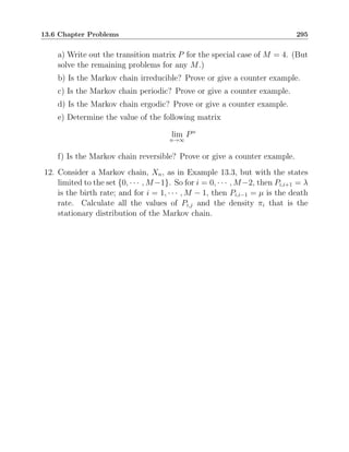


![300 General MRF Models
illustrated in Figure 14.1b. Notice, that any individual point, s ∈ S, forms a
clique with the single member, c = {s}.
In fact, cliques and neighborhood systems are alternative specifications
of the same information because for each neighborhood system, there is a
unique corresponding maximal set of cliques, and for each set of cliques there
is a unique corresponding minimal neighborhood system. (See problem 1)
With this definition of cliques, we may now define the concept of a Gibbs
distribution.
Definition 22. Gibbs Distribution
Let p(x) be the probability mass (density) function of a discrete (continuous)
valued random field Xs ∈ Ω defined on the lattice S with neighborhood system
∂s. Then we say that p(x) is a Gibbs distribution if it can be written in the
form
p(x) =
1
z
exp
(
−
X
c∈C
Vc(xc)
)
(14.1)
where z is a normalizing constant known as the partition function, C is
the set of all cliques, xc is the vector containing values of x on the set c, and
Vc(xc) is any functions of xc.
We sometimes refer to the function Vc(xc) as a potential function and
the function
u(x) =
X
c∈C
Vc(xc)
as the associated energy function.
The important result that relates MRFs and Gibbs distributions is the
Hammersley-Clifford Theorem[7] stated below.
Theorem 14.1.1. Hammersley-Clifford Theorem
Let S be an N point lattice with neighborhood system ∂s, and X be a dis-
crete (continuously) valued random process on S with strictly positive prob-
ability mass (density) function p(x) 0. Then X is an MRF if and only if
p(x) is a Gibbs distribution.
So the Hammersley-Clifford Theorem states that X is an MRF if and only
if its density function, p(x), is a Gibbs distribution. Since, Gibbs distributions
are restricted to be strictly positive, this result comes along with the technical](https://image.slidesharecdn.com/s6hfi7xht12wwcizuy0v-mbip-book-230123055619-8f2fce45/85/MBIP-book-pdf-310-320.jpg)


![308 General MRF Models
14.3 Discrete MRFs and the Ising Model
Perhaps the first serious attempts to generalize Markov chains to multiple di-
mensions came from the physics community in an effort to model the behavior
and properties of magnetic dipoles in real materials. Amazingly enough, some
of this early research resulted in closed form expressions for the behavior of
these highly non-linear systems, but they achieved this goal by restricting
their analysis to simple 2-D models with 4-point neighborhoods.
In the 1920’s, it was well known that magnetic materials exhibit a phase
transition when the temperature falls below the Curie temperature. Below
this critical temperature, the magnetic material will spontaneously mag-
netize itself, but above the critical temperature it will not. Wilhelm Lenz
[48] and his student, Ernst Ising [44], proposed what is now known as the
Ising model in an attempt to mathematically model this unique physical
behavior.
The Ising model is formed by a lattice of binary random variables that are
used to model the states of magnetic dipoles. Each binary variable, Xs, can
take on the value +1 or −1, indicating either a North or South orientation
of the corresponding dipole. The potential energy associated with a pair of
neighboring dipoles is then approximated as −Jxsxr where s ∈ ∂r and J
is a positive constant. So if the neighboring dipoles are misaligned, (i.e.,
xs = −xr), then the potential energy is J; and if they are aligned, (i.e.,
xs = xr), then the potential energy falls to −J. Using this model, the total
energy of the lattice is given by
u(x) = −
X
{s,r}∈C
Jxsxr ,
where C is the set of all neighboring pixel pairs (i.e., cliques).
The question that next arrises is, what is the distribution of the dipole
states in the Ising model? For a physical system, the question is answered
by the Boltzmann distribution (also known as the Gibbs distribution) of
thermodynamics. The Boltzmann distribution has the form
p(x) =
1
z
exp
−
1
kbT
u(x)
,
where u(x) is the energy associated with the state x. The Boltzmann distri-
bution is derived for a system in thermodynamic equilibrium by finding the](https://image.slidesharecdn.com/s6hfi7xht12wwcizuy0v-mbip-book-230123055619-8f2fce45/85/MBIP-book-pdf-318-320.jpg)
![14.3 Discrete MRFs and the Ising Model 309
distribution of states that maximizes the entropy of the system subject to a
constraint that the expected energy be constant. (See Appendix C and prob-
lem 6 for a derivation of this result.) So for the Ising model, the Boltzmann
distribution of states has the form
p(x) =
1
z
exp
1
kbT
X
{s,r}∈C
Jxsxr
. (14.6)
Since this is a Gibbs distribution, then we know that p(x) must be the dis-
tribution of an MRF with cliques given by C.
In order to be able to analyze the properties of this model, Ising first
assumed the lattice to be only one dimensional. Now we know from Sec-
tion 14.2 that any 1-D MRF of order P is a 1-D Markov chain of order P.
So this 1-D approximation allowed Ising to exactly analyze the behavior of
the lattice. However, in 1-D, the Ising model no longer exhibits the critical
temperature behavior! So let Xn be the 1-D random process resulting from
the Ising model, and assume that we know that X0 = 1. Then as n → ∞, we
know that the Markov chain will converge to a stationary distribution and
Xn will be independent of the initial value, X0. This means that in 1-D the
initial state has no lasting effect.
However, in 2-D, Gibbs distributions no longer can be represented as sim-
ple Markov chains. So the analysis is much more difficult, but also turns
out to yield much richer behavior. In fact in 1936, Peierls first provided a
precise argument that in 2-D the Ising model exhibits the expected critical
temperature behavior [58]. So below a specific critical temperature, dipoles
in the random field remain correlated regardless of how far apart they are.
Later this analysis was made more precise when in 1944 Onsager was able to
obtain a closed form expression for the infinite lattice case [55].
In order to better understand the Ising model, we first make the standard
modeling assumption of a 2-D rectangular lattice with a 4-point neighborhood
system, and cliques formed by neighboring horizontal or vertical pixel pairs.
If we use the notation, δ(xr 6= xs), as an indicator function for the event](https://image.slidesharecdn.com/s6hfi7xht12wwcizuy0v-mbip-book-230123055619-8f2fce45/85/MBIP-book-pdf-319-320.jpg)
![310 General MRF Models
xr 6= xs, then we can rewrite the Ising distribution in the form
p(x) =
1
z
exp
J
kbT
X
{r,s}∈C
xrxs
=
1
z
exp
J
kbT
X
{r,s}∈C
(1 − 2δ(xr 6= xs))
.
This results in a new expression for the distribution of an Ising model
p(x) =
1
z(β)
exp
−β
X
{r,s}∈C
δ(xr 6= xs)
, (14.7)
where
β ,
2J
kbT
(14.8)
is a standard parameter of the Ising model that is inversely proportional to
the temperature. Notice that we write z(β) to emphasize the dependence of
the partition function on β. Generally, it is more convenient and intuitive to
work with the unitless parameter of β than to work with the temperature T
directly.
From the form of (14.7), we know that p(x) is a Gibbs distribution with
pair-wise cliques. In 2-D, the Ising model uses horizontal and vertical cliques,
so by the Hammersly-Clifford Theorem, we also know that X must be a MRF
with a 4-point neighborhood. More directly, we can compute the conditional
distribution of a pixel xs given its neighbors xr for r ∈ ∂s to yield
p(xs|xi6=s) =
exp
−β
P
r∈∂s δ(xs 6= xr)
exp
−β
P
r∈∂s δ(1 6= xr) + exp
−β
P
r∈∂s δ(−1 6= xr)
.
(14.9)
In order to further simplify this expression, we can define v(xs, ∂xs) to be the
number of horizontal/vertical neighbors that differ from xs.
v(xs, x∂s) ,
X
r∈∂s
δ(xs 6= xr) (14.10)
From this we can compute the conditional probability that xs = 1 as
p(1|xi6=s) =
1
1 + e2β[v(1,x∂s)−2]
. (14.11)](https://image.slidesharecdn.com/s6hfi7xht12wwcizuy0v-mbip-book-230123055619-8f2fce45/85/MBIP-book-pdf-320-320.jpg)

![312 General MRF Models
- - - -
- - - -
- - - +
- - - +
- - - -
- + + -
+ + + -
+ - -
- - - -
- - - -
- - - -
- - - -
- + - -
+ + - -
- + - -
- - - -
+
Cliques: Xr Xs Xr
Xs
Boundary:
Figure 14.4: Example of a 2-D Ising models structure using a 4-point neighborhood.
In this case, the energy is proportional to the boundary length traced between pixels
of opposite sign.
sarily the case because as the length of a boundary increases the total number
of possible boundaries of a given length can increase quite rapidly.
The complex nature of the 2-D Ising model is perhaps best illustrated by
the existence of a critical temperature below which the correlations in the
lattice extend to infinite distances. Figure 14.5a illustrates an Ising model
of size N × N with a boundary specified by the set of lattice points B. So
one might expect that as the size the the lattice, N, tends to infinity, then
the choice of the boundary as either XB = 1 or XB = −1 would not affect
the pixels in the center of the lattice. However, this is not true. In 1936,
Peierls first showed this surprising result using a clever proof based on argu-
ments about the probability of a boundary surrounding the center pixel [58].
Kinderman and Snell provide a simplified example of this proof technique
on page 13 of [47] to show that for β sufficiently large the probability of the
center pixel, X0, can be made arbitrarily small. For β βc, it can be shown
that
lim
N→∞
P{X0 = −1|XB = 1} 1/2 .
In fact, by choosing β sufficiently large, it can be shown that limN→∞ P{X0 =
−1|XB = 1} ǫ for any ǫ 0. This means that the choice of a boundary
effects the behavior of the Ising model even as the boundary goes to infinity.
This is a behavior which is distinctly different than the behavior of a ergodic
1-D Markov chain, in which the effect of the initial value decays with time.
Example 14.1. In this example, we provide a simple geometric proof originally](https://image.slidesharecdn.com/s6hfi7xht12wwcizuy0v-mbip-book-230123055619-8f2fce45/85/MBIP-book-pdf-322-320.jpg)
![14.3 Discrete MRFs and the Ising Model 313
from Kinderman and Snell (See [47] page 13) that there exists a critical value,
βc, above which correlations in the lattice extend to infinite distances. The
proof works by first bounding the correlation for the case of an N ×N lattice,
and then taking the limit as N → ∞.
Figure 14.5a illustrates the situation in which an N × N Ising MRF has a
center pixel X0 which is surrounded by a outer boundary of values B. Our ob-
jective will be to show that for β sufficiently large, PN {X0 =−1|B =1} 1/3.
Once we have proven this, we than know that
lim
N→∞
PN {X0 =B} ≥ 2/3 ,
which means that the value of X0 and the boundary B are correlated re-
gardless of how large the lattice becomes. So intuitively, this center pixel of
the random field is affected by the boundary regardless of how far away the
boundary moves.
In order to formulate the proof, we will first need to define some notation.
Consider a particular configuration x for which x0 = −1 and B = 1. Then
we know there must be a closed boundary that surrounds the lattice point at
0 and that contains all the pixels with label −1 that are connected through
4-point neighbor relation to the pixel X0 = −1. This boundary and the
associated set of pixels inside the boundary are illustrated in Figure 14.5a.
Now let Ω = {+1, −1}N2
denote the set of all binary images, and let L(x)
be the total boundary length associated with neighboring pixels of opposite
polarity. Then the probability distribution of X given B = 1 has the form
P{X = x|XB = 1} =
1
z
exp {−βL(x)} .
Now let c(x) denote the closed boundary around the pixel X0 that includes
all pixels of value −1. Notice that all pixels inside the curve, c(x), must have
value −1, and all values immediately outside the curve must be +1.5
In
addition, since the outer boundary is assumed to be all 1′
s (i.e., B = 1) and
X0 = −1, then c(x) must exist as a separation between the change in these
two states. We will denote the length of this separating curve by L(c(x)).
Figure 14.5a) illustrates the situation with X0 = −1 and c(x) denoted by a
bold line of length L(c(x)) = 24 enclosing 15 pixels each with the value −1.
5
Of course, diagonal neighbors to the curve can be −1, and so can pixels that do not neighbor the curve.](https://image.slidesharecdn.com/s6hfi7xht12wwcizuy0v-mbip-book-230123055619-8f2fce45/85/MBIP-book-pdf-323-320.jpg)


![14.3 Discrete MRFs and the Ising Model 317
Amazingly, in 1944, Onsager was able to obtain closed form expressions
for properties of the Ising model as N → ∞ [55]. One representative result
from this analysis is the following expression for the conditional expectation
of a pixel in the lattice given that the boundary at infinity is XB = 1.
lim
N→∞
EN [X0|B = 1] =
(
1 − 1
(sinh(β))4
1/8
if β βc
0 if β βc
(14.14)
This expression, plotted in Figure 14.5b, clearly illustrates the critical tem-
perature behavior of the Ising model. For values of β below a critical value
of βc ≈ 0.88, the expected value of a pixel in the field is zero. This is what
you would expect if the effect of the boundary were to become negligible as
it tends towards infinity. However, for β βc (i.e., T Tc) where βc ≈ 0.88,
this symmetry is broken, and the expectation moves towards 1. In fact, for
large values of β, the expectation approaches 1, which means that X0 = 1
with high probability.
Intuitively, this happens because when β is above the critical value, the
random field’s distribution becomes bi-modal, tending to be either nearly
all values of 1 or nearly all values of −1. Clearly, without the boundary
condition, the probability of X and −X (i.e., the random field with the sign
of each pixel reversed) must be the same due to the symmetry in the density
of equation 14.6. However, the assumption of a boundary of B = 1 breaks
this symmetry in the model, and favors the mode associated with a majority
of 1’s in the lattice. In this case, values of −1 only occur in primarily isolated
locations.
The Ising model can be generalized to a wider range of similar models,
but typically in these more general cases, it is no longer possible to compute
closed form solutions to properties of the model. A simple and very useful
generalization of the Ising model is to an M-level discrete MRF with
typically an 8-point neighborhood. So for a 2-D lattice, let C1 denote the set
of horizontal and vertical cliques and let C2 denote the set of diagonal cliques.
Then we may define the following two statistics
t1(x) ,
X
{s,r}∈C1
δ(xr 6= xs) (14.15)
t2(x) ,
X
{s,r}∈C2
δ(xr 6= xs) , (14.16)](https://image.slidesharecdn.com/s6hfi7xht12wwcizuy0v-mbip-book-230123055619-8f2fce45/85/MBIP-book-pdf-327-320.jpg)
![318 General MRF Models
where t1(x) counts the number of vertically and horizontally adjacent pixels
with different values, t2(x) counts the number of diagonally adjacent pixels
with different values, and the pixels xs are assumed to take values in the set
{0, · · · , M − 1}. From this, we can express the distribution of an M-level
MRF as
p(x) =
1
z
exp {−(β1t1(x) + β2t2(x))} . (14.17)
We can also compute the conditional distribution of a pixel, Xs, given
its neighbors, X∂s. In order to compactly express this, we can first define
the functions v1 and v2 which count the number of horizontal/vertical and
diagonal neighbors with a different value from Xs. These functions are given
by
v1(xs, x∂s) ,
X
r∈[∂s]1
δ(xs 6= xr)
v2(xs, x∂s) ,
X
r∈[∂s]2
δ(xs 6= xr) ,
where [∂s]1 is the set of horizontally and vertically adjacent neighbors to s,
and [∂s]2 is the set of diagonally adjacent neighbors to s. Using this notation,
we can then express the conditional distribution of Xs given its neighbors as
p(xs|xr6=s) =
exp {−β1v1(xs, x∂s) − β2v2(xs, x∂s)}
PM−1
m=0 exp {−β1v1(m, x∂s) − β2v2(m, x∂s)}
.
In this form, it is clear that when β1, β2 0, the pixel Xs is more likely to
take on a value that is shared by a number of its neighbors.
14.4 2-D Markov Chains and MRFs
In Section 14.2, we showed that the 1-D Markov chain and 1-D MRF represent
equivalent models. Therefore, as a practical matter, a Markov chain model
is almost always preferred in 1-D since, in many ways, it is more tractable.
So this raises the question, are 2-D Markov chains and 2-D MRFs equiva-
lent? The answer to this is “no”. We will show that MRFs are more general
in two or more dimensions, or when the lattice forms a general graph rather
than a 1-D sequence or tree. In fact the relationship of Markov chains to](https://image.slidesharecdn.com/s6hfi7xht12wwcizuy0v-mbip-book-230123055619-8f2fce45/85/MBIP-book-pdf-328-320.jpg)


![324 General MRF Models
It is often the case that the Gibbs distribution is parameterized as an expo-
nential family so that it can be written as
uθ(x) = T(x)θ
where T(x) is a 1×k row vector and θ is a k ×1 column vector. For instance,
this is the case in the example of equation (14.17) where T(x) = [t1(x), t2(x)]
and θ = [β1, β2]t
. In this case, ∇uθ(x) = T(x), and the relationship of
equation (14.19) becomes
T(x) = Eθ̂ [T(X)] . (14.20)
Equation (14.20) has the intuitively appealing interpretation that, to compute
the ML estimate, one must adjust the components of the parameter θ until
the expected values of the statistics, (i.e., Eθ [T(X)]) match the observed
values of the statistics, (i.e., T(x)).
Of course, the difficulty in solving equation (14.20) is computing the re-
quired expectation. One approach to solving this problem numerically is
to approximately compute the expectation using the simulation techniques
of that will be introduced in Chapter 15. Methods such as the Metropo-
lis, Hastings-Metropolis, and Gibbs sampler provide techniques to generate
sequences of samples from the distribution of X using parameter θ. So for
example, simulation methods can be used to generate M samples from the
Gibbs distribution with the parameter θ. Then the following error can be
computed as
∆T ← T(x) −
1
M
M
X
m=1
T(X
(m)
θ ) ,
where {X
(m)
θ }M
m=1 are the M samples of X generated from the distribution
with parameter θ. Using this error, the parameters of θ can be adjusted by
decreasing its components in proportion to the error
θ ← θ − α∆T ,
where α is a user selected step size. In any case, this approach to ML es-
timation can be very computationally expensive since it requires the use of
stochastic sampling techniques, and its convergence can be fragile.
A much more commonly used approach to ML estimation for MRF pa-
rameters is the so called maximum pseudo-likelihood (MPL) estimator](https://image.slidesharecdn.com/s6hfi7xht12wwcizuy0v-mbip-book-230123055619-8f2fce45/85/MBIP-book-pdf-334-320.jpg)
![14.5 MRF Parameter Estimation 325
[8, 9]. The MPL estimator works by replacing the true likelihood with the so-
called pseudo likelihood that does not include the dreaded partition function.
Since X is a assumed to be an MRF, we know that it is possible to write the
conditional distributions of pixels given all other pixels as pθ(xs|x∂s), where
∂s is the set of neighbors to the pixel s. So the pseudo-likelihood function is
defined as
PL(θ) =
Y
s∈S
pθ(xs|x∂s) .
Of course, the pseudo-likelihood is not the actual likelihood because the
dependencies in the MRF are loopy. Nonetheless, we can use the pseudo-
likelihood as a criteria for optimization in parameter estimation. More specif-
ically, the maximum pseudo-likelihood estimate of the parameter θ is then
given by
θ̂ = arg max
θ
(
X
s∈S
log pθ(xs|x∂s)
)
So the maximum pseudo-likelihood estimate is based on the strategy of sim-
ply ignoring the loopy nature of the MRF dependencies and computing the
likelihood as if the probabilities formed a Markov chain.
However, one glitch in the approach is that in applications the parameter
θ typically is used to parameterize the Gibbs distribution rather than the
conditional probabilities themselves.7
So therefore, using the MPL approach
requires that the conditional distributions must be expressed in terms of the
associated Gibbs distribution using Bayes’ rule. This results in a complex and
typically nonlinear relationship between the parameters, θ, and the psuedo-
likelihood expression to be optimized. So consider a Gibbs distribution with
the form
pθ(x) =
1
z
exp
(
−
X
c∈C
Vc(xc|θ)
)
.
Once again, we can define Cs to be the set of all cliques that contain the pixel
xs. With this notation, it is easily shown that
pθ(xs|x∂s) =
exp
−
P
c∈Cs
Vc(xc|θ)
P
xs∈Ω exp
−
P
c∈Cs
Vc(xc|θ)
.
7
It is generally necessary to parameterize the Gibbs distribution rather than the conditional probabilities
because the Hammersley-Clifford Theorem does not say how to construct the full distribution from the con-
ditional distributions. Also, a given set of conditional distributions are not likely to consistently correspond
to any overall joint distribution.](https://image.slidesharecdn.com/s6hfi7xht12wwcizuy0v-mbip-book-230123055619-8f2fce45/85/MBIP-book-pdf-335-320.jpg)
![326 General MRF Models
So using this expression, the functional form of the maximum pseudo-likelihood
estimate is given by
θ̂ = arg max
θ
(
X
s∈S
log
exp −
P
c∈Cs
Vc(xc|θ)
P
xs∈Ω exp
−
P
c∈Cs
Vc(xc|θ)
!)
. (14.21)
While this expression is not very pretty, it can be numerically optimized. In
particular, it is tractable because the sum in the denominator of each term is
only over individual pixels, xs, rather than the entire MRF. However in prac-
tice, this expression tends to be a highly nonlinear function of the parameter
θ, so numerical optimization can be tricky. Nonetheless, an important advan-
tage of the maximum pseudo-likelihood estimate is that it has been shown to
be consistent [34], so it is typically better than completely ad-hoc parameter
estimates, which often are not.](https://image.slidesharecdn.com/s6hfi7xht12wwcizuy0v-mbip-book-230123055619-8f2fce45/85/MBIP-book-pdf-336-320.jpg)

![328 General MRF Models
a) Show that in 2-D the conditional distribution of a pixel given its
neighbors has the form of equation 14.11;
b) Plot the conditional probability p(xs = 1|xi6=s) as a function of
v(1, x∂s) with β = −1, 0, 0.5, and 1.
c) What would a “typical” sample of the X look like when β = −2?
8. Answer the following questions using results from Example 14.1 and
equation (14.14).
a) From the example, calculate a value of β which guarantees that
PN {X0 =−1|XB =1} 1/3 for all N 3.
b) Find a value of β which ensures that the limN→∞ EN [Xs|XB = 1] ≥
0.9 for all lattice points s.
c) Does the proof of Example 14.1 hold for a 1-D Ising model? If so,
prove the result. If not, explain why?
9. Let X be a binary valued 2-D random field with N × N points. Assume
that for 0 i, j ≤ N − 1
P{X(0,j) = 0} = P{X(i,0) = 0} =
1
2
and for
P{X(i,j) = x(i,j)|Xr = xr r (i, j)}
= g(x(i,j)|x(i−1,j), x(i,j−1))
=
1
3
δ(x(i,j), x(i−1,j)) +
1
3
δ(x(i,j), x(i,j−1)) +
1
6
a) Compute the complete density function for X.
b) Show that X is an MRF. Give the cliques and the neighborhood for
X.](https://image.slidesharecdn.com/s6hfi7xht12wwcizuy0v-mbip-book-230123055619-8f2fce45/85/MBIP-book-pdf-338-320.jpg)
![Chapter 15
Stochastic Simulation
So far, we have reviewed many non-causal image and signal models, and we
have shown how they can be of great value as prior distributions in inverse
problems such as image restoration and deconvolution. However, we have not
yet given any approach for generating samples from these distributions.
The objective of this chapter is to present a general class of techniques for
stochastic sampling from complex and high-dimensional distributions. These
techniques, which we broadly refer to as stochastic simulation, are based on
the use of Monte Carlo methods for pseudo-random sampling of distributions.
While we present stochastic simulation as a method for generating samples
of random objects, the methods can be used to simulate a broad range of
practical stochastic systems in applications ranging from signal processing,
to communications, to chemistry and material science. In addition, these
methods also serve as a basic tool used in a wide range of techniques including
stochastic optimization, stochastic integration, and stochastic EM parameter
estimation.
15.1 Motivation for Simulation Methods
In order to understand the motivation for stochastic simulation methods,
consider a situation in which one would like to use a computer to generate
a sample of a random variable X with a CDF of F(x) = P{X ≤ x}. The
classic approach to this problem is to first generate a pseudo-random number
which is uniformly distributed on the interval [0, 1],
U ← Rand([0, 1])](https://image.slidesharecdn.com/s6hfi7xht12wwcizuy0v-mbip-book-230123055619-8f2fce45/85/MBIP-book-pdf-339-320.jpg)
![330 Stochastic Simulation
where Rand([0, 1]) denotes a process for generating such a random variable.
Next, one calculates the inverse CDF defined by
F−1
(u) , inf{x|F(x) ≥ u} .
Then it can be shown that the desired random variable can be generated by
applying the inverse CDF to the uniform random variable.
X ← F−1
(U) (15.1)
In fact, it can be proven that this inverse transform sampling method
works for any random variable. (See problem 2 of Chapter 2)
With this result, one might think it would be easy enough to generate a
random variable with any desired distribution. However, this is not always
the case. For some distributions, like for example exponential or Gaussian
random variables,1
it is possible to calculate the inverse CDF in closed form,
so that the inverse transform method of equation (15.1) can be directly imple-
mented. However, for a general random variable, the inverse CDF typically
does not have any simple form; so that direct implementation is not tractable.
For example, consider the random variable, X, with a density function
given by
p(x) =
1
z
exp
n
−
4(x − 1)2
(x + 1)2
+
x
2
o
. (15.2)
where z is a normalizing constant for the density. In fact, this density has
the form of a Gibbs distribution, p(x) = 1
z e−u(x)
, where
u(x) = 4(x − 1)2
(x + 1)2
+
x
2
.
From Figure 15.1, we can see that both the energy function and its asso-
ciated density are bimodal for this distribution, with modes peaking at ap-
proximately x = ±1. Not surprisingly, the CDF of this density does not
have closed analytical form, so neither does its inverse. So how might one
efficiently generate samples of this random variable on a computer?
In the following sections, we present a set of tools broadly termed as
stochastic simulation methods, that can be used to generate samples from
1
It is interesting to note that the inverse CDF does not have closed form for the Gaussian distribution, but
this problem can be circumvented by generating the distribution of pairs of independent Gaussian random
variables since their vector norm is exponentially distributed.](https://image.slidesharecdn.com/s6hfi7xht12wwcizuy0v-mbip-book-230123055619-8f2fce45/85/MBIP-book-pdf-340-320.jpg)
![15.2 The Metropolis Sampler 331
−2 −1 0 1 2
0
1
2
Probability Density Function
−2 −1 0 1 2
0
10
20
30
Energy Function u(x)
Figure 15.1: Example of the energy function and density for a random variable with
the distribution specified in equation (15.2).
general distributions such as the one in equation (15.2). While we motivate
the method with this problem of generating a single random variable, the
technique has its greatest application in the generation of samples from very
complex high-dimensional distributions. As a matter of fact, the methods
were first introduced to generate samples from chemical systems in thermo-
dynamic equilibrium; so the approaches are quite generally useful.
The first subsection will introduce the Metropolis sampler, perhaps the
original example of a stochastic sampling method. Then we will extend this
approach to the more general Hastings-Metropolis sampler, and finally show
that the very useful Gibbs sampler is in fact a special case.
15.2 The Metropolis Sampler
The Metropolis sampler is a very clever method that allows samples to be
generated from any Boltzmann or equivalently Gibbs distribution [52]. Con-](https://image.slidesharecdn.com/s6hfi7xht12wwcizuy0v-mbip-book-230123055619-8f2fce45/85/MBIP-book-pdf-341-320.jpg)
![332 Stochastic Simulation
sider the discrete distribution on the set Ω with a PMF of the form2
p(x) =
1
z
exp {−u(x)} , (15.3)
where u(x) is an energy function and z is the associated partition function.
So any strictly positive PMF can be put in this form since it is always possible
to take the energy function as
u(x) = − log p(x) + const .
In fact, the random quantity X may be a random variable, or it may be a
higher dimensional random object such as a vector or random field.
The objective of a simulation algorithm is to generate a sequence of random
objects, denoted by X(k)
, whose distribution converges to the desired Gibbs
distribution, p(x). The strategy of the Metropolis algorithm is to use the
current sample, X(k)
, to generate a “proposal” for a new sample denoted by,
W. The proposal, W, is generated randomly, but its distribution is dependent
on the current sample, X(k)
. More specifically, the proposed sample W is
chosen from some conditional distribution q(w|X(k)
). However, this proposal
density, q(w|x(k)
), must obey the symmetry property that for all w, x ∈ Ω,
q(w|x) = q(x|w) . (15.4)
While the condition of (15.4) is quite restrictive, there are reasonable methods
for generating proposals that fulfill the condition. For example, we can set
the proposal to be W ← X(k)
+ Z, where Z is a random variable with a
symmetric PDF that is independently generated at each new time k. In this
case, it is easy to show that the condition applies.
In practice, the proposal W can be generated with the inverse transform
sampling method of equation (15.1). In pseudocode, this can be expressed as
U ← Rand([0, 1])
W ← Q−1
(U|X(k)
) ,
where Q−1
(·|x(k)
) is the inverse CDF corresponding to the density q(w|x(k)
).
The proposal density is typically chosen to be relatively simple, so that gen-
erating samples from this distribution is easy.
2
The theory we develop here assumes discrete random variables, but the methods equally apply to the
sampling of continuously valued random variables. In fact, the extension to continuous random variable is
largely intuitive since the continuous random variables can be quantized to form discrete ones.](https://image.slidesharecdn.com/s6hfi7xht12wwcizuy0v-mbip-book-230123055619-8f2fce45/85/MBIP-book-pdf-342-320.jpg)
![15.2 The Metropolis Sampler 333
The clever trick of the Metropolis algorithm is then to accept or reject
these proposals in a very particular way. To do this, we first compute the
change in the energy given by ∆E ← u(W)−u(X(k)
). If the change in energy
is negative, ∆E 0, then we immediately accept the proposal, so that
X(k+1)
← W if ∆E 0 .
However, if the change in energy is positive, ∆E ≥ 0, then we accept the
proposal with a probability of e−∆E
and reject it with probability 1 − e−∆E
.
In practice, this is done with the following two steps.
U ← Rand([0, 1])
X(k+1)
← W if ∆E ≥ 0 and U e−∆E
X(k+1)
← X(k)
if ∆E ≥ 0 and U ≥ e−∆E
.
We can simplify this acceptance decision by introducing a function that
expresses the acceptance probability for each proposal.
α(w|x(k)
) = min
n
1, e−[u(w)−u(x(k)
)]
o
(15.5)
Using this function, the Metropolis sampling is performed in the following
steps. First, the proposal, W, is generated according to the sampling distri-
bution.
U ← Rand([0, 1])
W ← Q−1
(U|X(k)
)
Then the sample is either accepted or rejected according to the acceptance
probability α(W|X(k)
).
U ← Rand([0, 1])
X(k+1)
← W if U α(W|X(k)
)
X(k+1)
← X(k)
if U ≥ α(W|X(k)
) .
Figure 15.2 lays out the Metropolis algorithm in pseudocode format. The
intuition behind the algorithm is that decreases in energy are always ac-
cepted but the probability of accepting a proposal with an increasing energy
decreases exponentially as the energy increases.](https://image.slidesharecdn.com/s6hfi7xht12wwcizuy0v-mbip-book-230123055619-8f2fce45/85/MBIP-book-pdf-343-320.jpg)
![334 Stochastic Simulation
Metropolis Algorithm:
Initialize X(0)
For k = 0 to K − 1 {
/*Generate proposal*/
W ∼ q(w|X(k)
) /*Use proposal distribution to generate W*/
/*Accept or reject proposal*/
α ← min
n
1, e−[u(W)−u(X(k))]
o
/*Compute acceptance probability*/
X(k+1)
←
W with probability α
X(k)
with probability 1 − α
}
Figure 15.2: A pseudocode specification of the Metropolis algorithm for stochastic
simulation from Gibbs distributions.
While this may all seem reasonable, how do we know that the Metropolis
algorithm converges to the desired distribution of equation (15.3)? The proof
of convergence depends on a clever use of ergodic theory for Markov chains.
First notice that the sequence {X(k)
}N
k=1 is a Markov chain. This is because
each new sample, X(k+1)
, is only dependent on the previous sample, X(k)
,
and other independently generated random variables.
Next, we can show (perhaps surprisingly) that this Markov chain is re-
versible as defined in Section 13.4. To see why this is true, consider the
transition probabilities for the Markov chain denoted by p(x(k+1)
|x(k)
). With
a little thought it is clear that the transition probability is given by
p(x(k+1)
|x(k)
) =
(
q(x(k+1)
|x(k)
)α(x(k+1)
|x(k)
) if x(k+1)
6= x(k)
1 −
P
w6=x(k) q(w|x(k)
) α(w|x(k)
) if x(k+1)
= x(k)
. (15.6)
The justification for this expression is that when x(k+1)
6= x(k)
, then the
probability of the transition is the product of the probabilities that you will
generate the proposal multiplied by the probability that you will accept the
proposal. Of course, since the transition probabilities must sum to one, the
probability that x(k+1)
= x(k)
is just one minus the sum of the alternative
cases.
In order to show that these transition probabilities are reversible, we must
show that for all state combinations, (x, x′
), the detailed balance equations](https://image.slidesharecdn.com/s6hfi7xht12wwcizuy0v-mbip-book-230123055619-8f2fce45/85/MBIP-book-pdf-344-320.jpg)
![15.2 The Metropolis Sampler 335
of (13.29) hold. For our problem, these are given by
p(x′
|x)
1
z
e−u(x)
= p(x|x′
)
1
z
e−u(x′
)
,
where p(x) = 1
z e−u(x)
is the stationary distribution of the ergodic Markov
chain.
To show this, we will consider three cases: case 1 in which u(x′
) ≤ u(x)
and x′
6= x; case 2 in which u(x′
) u(x) and x′
6= x; and case 3 in which
x′
= x. For case 1, we have have that
p(x′
|x) = q(x′
|x) α(x′
|x)
= q(x′
|x)
= q(x|x′
)
= q(x|x′
) e−[u(x)−u(x′
)]
e[u(x)−u(x′
)]
= q(x|x′
) α(x|x′
) e[u(x)−u(x′
)]
= p(x|x′
) e[u(x)−u(x′
)]
. (15.7)
Rearranging terms and normalizing by the partition function z then provides
the desired result.
p(x′
|x)
1
z
e−u(x)
= p(x|x′
)
1
z
e−u(x′
)
(15.8)
Now there are two additional cases to consider. Case 2 results from swap-
ping the roles of x and x′
. However, the symmetry of equation (15.8) then
immediately yields the desired result. For case 3, substituting in x = x′
results in the two sides of equation (15.8) being identical; so the required
equality holds trivially.
The detailed balance equations of (15.8), then imply the full balance equa-
tions hold by simply summing over the variable x.
X
x∈Ω
p(x′
|x)
1
z
e−u(x)
=
1
z
e−u(x′
)
(15.9)
So we can see that the Gibbs distribution p(x) = 1
z e−u(x)
is in fact the station-
ary distribution of the Markov chain generated by the Metropolis algorithm.
By Theorem 13.4.1 of Section 13.4, we now know that if the proposal
distribution q(x(k+1)
|x(k)
) is chosen so that all states can be accessed (i.e.,](https://image.slidesharecdn.com/s6hfi7xht12wwcizuy0v-mbip-book-230123055619-8f2fce45/85/MBIP-book-pdf-345-320.jpg)
![336 Stochastic Simulation
Hastings-Metropolis Algorithm:
Initialize X(0)
For k = 0 to K − 1 {
/*Generate proposal*/
W ∼ q(w|X(k)
) /*Use proposal distribution to generate W*/
/*Accept or reject proposal*/
α ← min
1,
q(X(k)
|W)
q(W|X(k))
exp
−[u(W) − u(X(k)
)]
/*Acceptance prob.*/
X(k+1)
←
W with probability α
X(k)
with probability 1 − α
}
Figure 15.3: A pseudocode specification of the Hastings-Metropolis algorithm for
stochastic simulation from Gibbs distributions. The Hastings-Metropolis algorithm
improves on the more basic Metropolis algorithm by allowing for an asymmetric
proposal distribution.
the Markov chain is irreducible), the probability of remaining in the same
state is greater than zero (i.e., the Markov chain is aperiodic), and if the
number of states are finite, then the Metropolis algorithm must generate an
ergodic Markov chain that converges to the desired Gibbs distribution.
In this case, we have that
lim
k→∞
P{X(k)
= x} =
1
z
exp{−u(x)} .
In fact, the Metropolis algorithm is commonly used even when these tech-
nical conditions do not hold. For example, it is commonly used to generate
samples from high-dimensional continuous distributions with densities, such
as non-Gaussian MRF models like those discussed in Chapter 6. In fact,
much stronger convergence results exist for stochastic simulation methods
and ergodic Markov chains, so our convergence result is simply provided to
illustrate the basic concept.
15.3 The Hastings-Metropolis Sampler
While the Metropolis algorithm is a very powerful method, it can be slow
to converge to the desired distribution. This is a problem for two important](https://image.slidesharecdn.com/s6hfi7xht12wwcizuy0v-mbip-book-230123055619-8f2fce45/85/MBIP-book-pdf-346-320.jpg)
![15.3 The Hastings-Metropolis Sampler 337
reasons. First, it means that one might need to generate many samples be-
fore the ergodic distribution is reached. This time need to run the Markov
chain until it approximately converges to its ergodic distribution is some-
times referred to as the burn-in time. But a second equally important
consequence of slow convergence is that it requires more samples to be gen-
erated before the random variables Xk
become approximately independent.
Naive users sometime assume that subsequent samples of the Markov chain
are independent, but this is not true. So if the object is to produce inde-
pendent stochastic samples from the Markov chain, as is often the case, then
a slowly converging Markov chain will require more samples between each
approximately independent sample.
A crucial limitation in the Metropolis algorithm is the requirement that
the proposal distribution be symmetric. That is
q(x(k+1)
|x(k)
) = q(x(k)
|x(k+1)
) .
Intuitively, it is best if the proposal distribution closely approximates the
desired ergodic distribution. However, this restriction to a symmetric distri-
bution is severe because it is often the case that we might want to “bias”
the proposals towards ones that more closely match the desired distribution
and are therefore more likely to be accepted.3
Intuitively, proposals that are
rejected do not lead to any change in the state, so they are substantially
wasted, and one would expect the associated Markov chain’s convergence to
be slowed [38].
Fortunately, Hastings and Peskun discovered a generalization of the Metropo-
lis sampler, generally referred to as the Hastings-Metropolis sampler,
that allows for the use of proposal distributions that are not symmetric
[40, 59]. So in this case, any valid distribution, q(xk
|xk−1
), can be chosen,
but in order to correct for the bias due to this asymmetric proposal density,
the probability of acceptance and rejection must be appropriately adjusted.
The acceptance probability for the Hastings-Metropolis sampler is given
3
This strategy is also highly recommended when pursuing funding.](https://image.slidesharecdn.com/s6hfi7xht12wwcizuy0v-mbip-book-230123055619-8f2fce45/85/MBIP-book-pdf-347-320.jpg)
![338 Stochastic Simulation
by
α(w|x(k)
) = min
1,
q(x(k)
|w)
q(w|x(k))
exp
n
−[u(w) − u(x(k)
)]
o
= min
1,
q(x(k)
|w)
q(w|x(k))
p(w)
p(x(k))
.
So the resulting transition probability is then given by
p(x(k+1)
|x(k)
) =
(
q(x(k+1)
|x(k)
)α(x(k+1)
|x(k)
) if x(k+1)
6= x(k)
1 −
P
w6=x(k) q(w|x(k)
) α(w|x(k)
) if x(k+1)
= x(k)
.
(15.10)
As with the basic Metropolis algorithm, our approach is to prove that the
Markov chain resulting from the Hastings-Metropolis algorithm is reversible.
To prove this, we must again show that the Gibbs distribution solves the
detailed balance equation. Our proof is broken into three cases:
Case 1: x′
6= x and q(x|x′
)
q(x′|x) exp {−[u(x′
) − u(x)]} ≥ 1;
Case 2: x′
6= x and q(x|x′
)
q(x′|x) exp {−[u(x′
) − u(x)]} ≤ 1;
Case 3: x′
= x.
We again start with case 1 for which we have that
p(x′
|x) = q(x′
|x) α(x′
|x)
= q(x′
|x)
= q(x|x′
)
q(x′
|x)
q(x|x′)
= q(x|x′
)
q(x′
|x)
q(x|x′)
exp{−[u(x) − u(x′
)]} exp{−[u(x′
) − u(x)]}
= q(x|x′
) α(x|x′
) exp{−[u(x′
) − u(x)]}
= p(x|x′
) exp{−[u(x′
) − u(x)]} , (15.11)](https://image.slidesharecdn.com/s6hfi7xht12wwcizuy0v-mbip-book-230123055619-8f2fce45/85/MBIP-book-pdf-348-320.jpg)

![340 Stochastic Simulation
−2 −1 0 1 2
0
1
2
Probability Density Function
−2 −1 0 1 2
0
1
2
Proposal Density Function
0 10 20 30 40 50
−2
0
2
Metropolis Sample Values
0 10 20 30 40 50
−2
0
2
Hastings−Metropolis Sample Values
Figure 15.4: Example illustrating the use of the Metropolis and Hastings-Metropolis
algorithms for stochastic sampling of a random variable. (upper left) Plot of the
desired density function of equation (15.13); (upper right) Time sequence of sample
values generated by the Metropolis algorithm. (lower left) Plot of the proposal density
function formed by a mixture of two Gaussians. (lower right) Time sequence of
sample values generated by the Hastings-Metropolis algorithm. Notice that adjacent
samples generated by the Metropolis algorithm are often the same because the updates
are rejected. Alternatively, the proposals of the Hastings-Metropolis are more often
accepted, leading to faster convergence of the Markov chain.
where σ = 1/2. So therefore, we see that the proposal density has the
symmetry property required for the Metropolis algorithm.
q(w|x(k)
) = q(x(k)
|w)
The acceptance probability is then given by
α = min
n
1, exp{−[u(w) − u(x(k)
)]}
o
= min
1,
p(w)
p(x(k))
.
The time sequence of values generated by the Metropolis algorithm is
shown in the upper right hand plot of Figure 15.4. Notice that sequential
values are often exactly the same. This is because many of the samples are
rejected. Intuitively, this high rejection rate slows down convergence of the
Markov chain.
Next, we use the Hasting-Metropolis algorithm to generate samples. For
this algorithm, we are not limited to symmetric proposal densities, so we may
very roughly approximate the desired distribution of equation (15.13). We
do this rough approximation with a mixture of two Gaussian distributions,](https://image.slidesharecdn.com/s6hfi7xht12wwcizuy0v-mbip-book-230123055619-8f2fce45/85/MBIP-book-pdf-350-320.jpg)
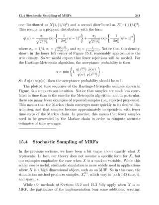
![342 Stochastic Simulation
More specifically, one needs to consider what practical choices exist for the
proposal distribution, q(w|x).
When X is high dimensional, it is common to restrict the proposals to
changes in only one coordinate of the high dimensional vector. So for example,
the proposal distribution is restricted to have the form
qs(w|x) = gs(ws|x) δ(wr − xr; r 6= s) , (15.14)
where gs(ws|x) is the conditional proposal distribution of a single pixel, Ws,
given the random field X. The term δ(wr − xr; r 6= s) in the conditional
probability indicates that all other pixels remain the same. So Wr = Xr for
r 6= s. We refer to this strategy of only replacing a single pixel at a time as
a coordinate-wise sampler.
Pseudocode for the corresponding coordinate-wise Hastings-Metropolis al-
gorithm is listed in Figure 15.5. Notice that the pixels in the MRF are first
ordered from 0 to N − 1, and this ordering is denoted by {si}N−1
i=0 . Then in
a single full iteration through the image, the pixels are visited and updated
in this repeating sequence. For this case, the acceptance probability is then
given by
α = min
1,
qsi
(X(k)
|W)
qsi
(W|X(k))
exp
n
−[u(W) − u(X(k)
)]
o
(15.15)
= min
(
1,
gsi
(X
(k)
si |W)
gsi
(Wsi
|X(k))
exp
n
−[u(W) − u(X(k)
)]
o
)
. (15.16)
Now if the 1-D density function gs(ws|x) 0 for all ws and x, then on each
update it is possible (but perhaps not very likely) to produce any pixel update.
And since in one pass through the pixels of X, every pixel is updated, then
in a single update any new image is possible. This means that the resulting
Markov chain is both irreducible and aperiodic Moreover, assuming that the
Hastings-Metropolis method is used to accept or reject proposals, then the
Markov chain will also be reversible. So we know that with the update of
any pixel, s, the detailed-balance equations must be satisfied; and therefore,
the full-balance equations must also be satisfied by the Gibbs distribution.
1
z
e−u(x(k+1)
)
=
X
x(k)∈ΩN
ps(x(k+1)
|x(k)
)
1
z
e−u(x(k)
)](https://image.slidesharecdn.com/s6hfi7xht12wwcizuy0v-mbip-book-230123055619-8f2fce45/85/MBIP-book-pdf-352-320.jpg)
![15.4 Stochastic Sampling of MRFs 343
Coordinate-Wise Hastings-Metropolis Algorithm:
Initialize X(0)
Select ordering of pixels, {si}N−1
i=0
Initialize k ← 0
For l = 0 to L − 1 { /* Repeat for L full iterations through the MRF */
For i = 0 to N − 1 {
/*Generate proposal*/
W ← X(k)
/*Initialize proposal*/
Wsi
∼ gsi
(w|X(k)
) /*Proposal for sth
i pixel*/
/*Accept or reject proposal*/
α ← min
(
1,
gsi
(X
(k)
si |W)
gsi
(Wsi
|X(k))
exp
−[u(W) − u(X(k)
)]
)
X(k+1)
←
W with probability α
X(k)
with probability 1 − α
k ← k + 1
}}
Figure 15.5: A pseudocode for a Hastings-Metropolis sampler using coordinate-wise
updates. The pseudocode performs L complete iterations through the full MRF, and
each full iteration performs a single update of each pixel. The resulting Markov chain
is nonhomogeneous, but it still convergences to the desired Gibbs distribution.
However, the analysis of the previous section assumed that the proposal
distribution, q(x(k+1)
|x(k)
), is fixed. But in this case, the proposal distribution
of equation (15.14) is dependent on s, the pixel being updated. Therefore,
the resulting Markov chain is not homogeneous. Since it is not homogeneous,
it is also unclear as to whether it converges to the desired Gibbs distribution.
Nonetheless, it seems intuitively clear that if the pixels are updated in a
fixed and repeated order, then the Markov chain should converge. The fol-
lowing argument confirms this intuition. From Property 13.2 of Chapter 13,
we know that the subsampling of any Markov chain produces another Markov
chain. So let X(k)
be the state after k updates. The subsampled version is
then Y (k)
= X(Nk)
where N is the number of pixels in the image. Then
Y (0)
= X(0)
is the initial state, Y (1)
= X(N)
is the state after a single update
of each pixel, and Y (k)
= X(Nk)
is the result after k full updates of the state.
Now Y (k)
is a Markov chain because it is formed by a subsampling of X(k)
.](https://image.slidesharecdn.com/s6hfi7xht12wwcizuy0v-mbip-book-230123055619-8f2fce45/85/MBIP-book-pdf-353-320.jpg)

![15.5 The Gibbs Sampler 345
always converges to the desired result. However, in some cases, this conver-
gence can be very slow.
Moreover, this theorem also guarantees convergence of the basic-Metropolis
algorithm, since that is a special case. Another special case, that is widely
used in practice, is the so-called Gibbs sampler presented in the following
section.
15.5 The Gibbs Sampler
Gibbs Sampler Algorithm:
Initialize X(0)
Select ordering of pixels, {si}N−1
i=0 /* Can use raster order */
Initialize k ← 0
For l = 0 to L − 1 {
For i = 0 to N − 1 {
/*Generate update for sth
i pixel*/
X(k+1)
← X(k)
/*Initialize update*/
Wsi
∼ gsi
(wsi
|X
(k)
∂si
) /* Generate sample from conditional distrib.*/
X
(k+1)
si ← Wsi
/* Replace pixel with generated sample */
k ← k + 1
}}
Figure 15.6: The Gibbs sampler algorithm is a special case of the coordinate-wise
Hastings-Metropolis algorithm when the proposal distribution for each pixel is just
its conditional distribution given its neighbors, i.e., X
(k+1)
s ∼ ps(xs|X
(k)
∂s ). In this
case, the acceptance probability is always α = 1; so all proposals are accepted.
The Gibbs sampler is an important special case of the coordinate-wise
Hastings-Metropolis sampler that was first proposed by Geman and Geman
[33] and has since become widely used due to its ease of implementation and
relatively fast convergence for simple distributions. With the Gibbs sampler,
the proposal distribution is taken to be the conditional distribution of the
pixel Xs given its neighbors under the Gibbs distribution.](https://image.slidesharecdn.com/s6hfi7xht12wwcizuy0v-mbip-book-230123055619-8f2fce45/85/MBIP-book-pdf-355-320.jpg)
![346 Stochastic Simulation
Assume that X is an MRF4
with a Gibbs distribution of the form
p(x) =
1
z
exp {−u(x)}
=
1
z
exp
(
−
X
c∈C
Vc(xc)
)
,
where u(x) is the energy function and Vc(xc) are the potential functions for
clique c. If we again define Cs from equation (14.2) to be the subset of all
cliques containing xs, then we know from equation (14.3) that the conditional
distribution of a pixel, xs, given all other pixels has the form
P{Xs = xs|Xr r 6= s} =
exp {−us(xs|x∂s)}
P
xs∈Ω exp {−us(xs|x∂s)}
where
us(xs|x∂s) =
X
c∈Cs
Vc(xc) .
So then for a Gibbs sampler, the key idea is to use the conditional distri-
bution of a pixel as the proposal distribution. More specifically, the proposal
distribution is given by
gs(xs|x∂s) = P{Xs = xs|Xi = xi i 6= s}
=
exp{−us(xs|x∂s)}
X
x′
s∈Ω
exp{−us(x′
s|x∂s)}
.
In this case, the acceptance probability can be computed in closed form to
be
α = min
(
1,
gs(X
(k)
s |W∂s)
gs(Ws|X
(k)
∂s )
exp
n
−[u(W) − u(X(k)
)]
o
)
= min
1,
gs(X
(k)
s |W∂s)
gs(Ws|X
(k)
∂s )
exp
n
−u(Ws|X
(k)
∂s )
o
exp
n
−u(X
(k)
s |X
(k)
∂s )
o
= min {1, 1} = 1 . (15.17)
4
Without loss of generality, X can be assumed to be an MRF because we can always take ∂s = {r : r 6= s}.](https://image.slidesharecdn.com/s6hfi7xht12wwcizuy0v-mbip-book-230123055619-8f2fce45/85/MBIP-book-pdf-356-320.jpg)


![356 Bayesian Segmentation
Xs is
pys|xs
(ys|m, φ) =
J−1
X
j=0
πm,j|Bm,j|1/2
(2π)p/2
exp
−
1
2
(ys − µm,j)t
Bm,j(ys − µm,j)
,
(16.3)
and the negative log likelihood is given by
l(ys|m, φ) = (16.4)
− log
J−1
X
j=0
πm,j|Bm,j|1/2
(2π)p/2
exp
−
1
2
(ys − µm,j)t
Bm,j(ys − µm,j)
!
.
Once forward and prior models have been chosen, we can apply some
type of Bayesian estimator to determine X from Y . The general approach,
described in Section (2.3.2), is to select a cost function, C(x, x̂), and then
choose the estimator X̂ = T(Y ) that minimizes the expected cost.
T∗
= arg min
T
E[C(X, T(Y )]
If the cost is chosen to be C(x, x̂) = 1 − δ(x − x̂), then the optimal estimator
is the MAP estimate given by
X̂ = T∗
(Y )
= arg max
x∈ΩN
px|y(x|Y )
= arg min
x∈ΩN
− log py|x(Y |x) − log p(x) . (16.5)
However, the cost function of the MAP estimate is difficult to justify since
it is only 0 when there is an exact match between the true segmentation
X and the estimate X̂. This is a very conservative criteria since it means
that having one erroneous pixel classification is no worse then having every
pixel wrong. Nonetheless, the MAP estimate is widely used because it can be
implemented with numerical optimization, and it often yields good results.
A more compelling cost criteria actually counts the number of classification
errors in the image, rather than simply checking to see if the classification is
perfect. This cost function is given by
C(x, X) =
X
s∈S
δ(xs 6= Xs) ,](https://image.slidesharecdn.com/s6hfi7xht12wwcizuy0v-mbip-book-230123055619-8f2fce45/85/MBIP-book-pdf-366-320.jpg)
![16.1 Framework for Bayesian Segmentation 357
and minimization of this cost function results in the so-called maximizer of
the posterior marginals (MPM) estimator [51] given by
X̂s = arg max
xs
pxs|Y (xs|Y ) . (16.6)
This MPM estimator has the property that it minimizes the number of mis-
classified pixels in the image, which is quite reasonable in most applications,
but it has the disadvantage that it requires the computation of an (N − 1)-
dimensional integral or expectation.
X̂s = arg max
xs
E
py|x(Y |xs, Xr r 6= s)p(xs, Xr r 6= s)|Y
(16.7)
While computing this high-dimensional integral for each pixel might seem
impossible, it can be done using the stochastic sampling techniques of Chap-
ter 15 as we will describe in Section 16.1.2.
In the following sections, we will introduce some of the methodologies for
computing Bayesian estimates of discrete random fields, X, with a structure
as shown in Figure 16.1. In particular, we will present basic methods for
computing both the MAP and MPM estimates of equations (16.5) and (16.7).
16.1.1 Discrete Optimization for MAP Segmentation
In order to illustrate basic methods for optimization of the MAP cost func-
tion, we start by assuming that the image has a log likelihood with a product-
form as in equation (16.1) and a prior model based on an M-level discrete
MRF. Then the negative log likelihood is given by
− log py|x(y|x) = −
X
s∈S
log pys|xs
(ys|xs)
=
X
s∈S
l(ys|xs) ,
where l(ys|xs) = − log pys|xs
(ys|xs) is the negative log likelihood for each pixel,
and the negative log prior term is given by
− log p(x) = β
X
{s,r}∈C
δ(xr 6= xs) + const ,](https://image.slidesharecdn.com/s6hfi7xht12wwcizuy0v-mbip-book-230123055619-8f2fce45/85/MBIP-book-pdf-367-320.jpg)
![358 Bayesian Segmentation
where C contains all pairwise cliques in an 8-point neighborhood. Using these
two models, the MAP estimate is given by
x̂ = arg min
x∈ΩN
− log py|x(y|x) − log p(x)
= arg min
x∈ΩN
X
s∈S
l(ys|xs) + β
X
{s,r}∈C
δ(xr 6= xs)
. (16.8)
In general, optimization problems with the form of equation (16.8) are very
difficult to solve. Since they are discrete, they certainly can not be convex.
In fact, even the definition of convexity no longer applies since it requires
the function to be defined along any line connecting two inputs values to the
function, and a linear combination of two discrete variables is not necessarily
discrete.
In general this optimization problem will have exponential complexity.
However, in the special case when M = 2, this type of optimization can be
solved exactly in polynomial time by using graph cut algorithms based on
the max-flow min-cut theorem [39]. This class of graph cut algorithms can
be solved in polynomial time by the Ford-Fulkerson algorithm [27]. In
fact, this approach works for any problem with the form of equation (16.8)
when M = 2. Moreover, it even holds when the neighborhoods have arbitrary
structure and the weights of the potential function are space varying. So for
example, it works for binary segmentation using the M-level discrete MRF
of equation (14.17) with M = 2.
However, the exact graph-cut solution does not work when M 2, and it
generally only works when the log likelihood of the data has a simple product
form of equation (16.1). In particular, the product form is often not a realistic
assumption when pixels are conditionally dependent or depend on the class
label of nearby pixels. Nonetheless, graph-cut algorithms have become very
popular in image segmentation, so these can be a very useful technique [18].
So absent an exact algorithm for minimization of equation (16.8), we must
resort to some approximate method of minimization. Early on, there were
many attempts to use dynamic programming to solve this MAP segmentation
problem in much the same way that dynamic programming can be used to
solve the MAP estimation problem for HMMs. However, dynamic program-
ming does not work in 2-D because the state variable must have the dimension](https://image.slidesharecdn.com/s6hfi7xht12wwcizuy0v-mbip-book-230123055619-8f2fce45/85/MBIP-book-pdf-368-320.jpg)
![16.1 Framework for Bayesian Segmentation 359
of an entire row or column of the image, which makes the complexity expo-
nential. Nonetheless, various approximation methods have been proposed for
doing approximate MAP segmentation by, for example, processing a small
number of image rows at a time [21, 80].
Perhaps the most common approach to minimization of this cost function
is coordinate-wise optimization similar to ICD. For discrete random fields, X,
this approach is often called iterated conditional modes (ICM) [9]. ICM
works by iteratively replacing each pixel’s class with the class that maximizes
the mode of the conditional distribution p(xs|y, xr r 6= x). This can be
computed as
x̂s ← arg max
xs
p(xs|y, xr r 6= s)
= arg min
xs
− log py|x(y|xs, xr r 6= s) − log p(xs, xr r 6= s)
= arg min
xs
{l(ys|xs) − log p(xs, xr r 6= s)}
= arg min
xs
l(ys|xs) + β
X
{i,j}∈C
δ(xi 6= xj)
= arg min
xs
(
l(ys|xs) + β
X
r∈∂s
δ(xs 6= xr)
)
.
So with this, we see that replacing each pixel with its conditional mode is
exactly equivalent to performing an ICD update, i.e., sequentially replacing
each pixel with the value that maximizes the MAP cost function. So ICD
and ICM are equivalent for discrete random fields, X.
Figure 16.2 provides a pseudocode specification of the ICM algorithm. The
segmentation is initialized with the ML estimate of the class of each pixel.
This is simply the class that maximizes the likelihood for each observation Ys.
Then for each iteration of the algorithm, every pixel is visited and replaced
with the class that maximizes the MAP cost function. This can be done with
little computation since each pixel is only dependent on the local negative
log likelihood, l(ys|xs), and the class of its neighbors. Each pixel replacement
monotonically decreases the MAP cost function, and the MAP cost function is
bounded below, so this sequence is guaranteed to converge to a local minimum
of the cost function in a finite number of steps. When this happens, each](https://image.slidesharecdn.com/s6hfi7xht12wwcizuy0v-mbip-book-230123055619-8f2fce45/85/MBIP-book-pdf-369-320.jpg)


![16.1 Framework for Bayesian Segmentation 363
SA Algorithm:
Initialize with ML estimate xs ← arg min0≤mM l(ys|m)
Select an annealing schedule: Decreasing sequence Tk
For k = 1 to ∞ {
For each pixel s ∈ S {
Compute the conditional energy
u(xs|xr r 6= s) = l(ys|xs) + β
X
r∈∂s
δ(xr 6= xs)
Generate a new pixel
xs ∼
exp
n
1
Tk
u(xs|xr r 6= s)
o
PM−1
m=0 exp
n
1
Tk
u(m|xr r 6= s)
o
}
}
Figure 16.3: A pseudocode specification of the SA algorithm for computing an ap-
proximate MAP estimate of a discrete random field X. The SA algorithm has the
advantage that it can avoid local minima in the MAP cost function, but at the cost
of often substantial additional computation.
answered by Geman and Geman in their classic paper [33]; however, the an-
swer is perhaps still unsatisfying. Let N be the number of pixels in X, and
define ∆ = maxx u(x)−minx u(x). Then an annealing schedule with the form
Tk =
N∆
log(k + 1)
,
produces an sequence of Gibbs samples X(k)
that converge to the MAP es-
timate x̂ almost surely [33]. However, the problem is that this annealing
schedule is absurdly slow. In fact, for this reason has been said that “SA
minimization is only slightly worse than exhaustive search.”3
For example,
if N = 10,000 and ∆ = 1, then in order to achieve a temperature of Tk = 1
corresponding to simply sampling form the posterior distribution requires a
number of simulation steps of k ≥ e10,000
− 1. This is completely impractical!
So in practice, people use SA but with much faster annealing schedules
that allow for some type of reasonable tradeoff between speed and accuracy.
For example, a more typical annealing schedule that achieves a reasonable
3
This insightful statement was reported to have been made by Allan Willsky.](https://image.slidesharecdn.com/s6hfi7xht12wwcizuy0v-mbip-book-230123055619-8f2fce45/85/MBIP-book-pdf-373-320.jpg)


![16.1 Framework for Bayesian Segmentation 367
Stochastic MPM Algorithm:
/* Generate L samples from the posterior distribution */
For l = 1 to L − 1 {
Generate a stochastic sample from the distribution
X(l)
∼
1
z
exp {−u(x)}
where u(x) =
X
s∈S
l(ys|xs) + β
X
{s,r}∈C
δ(xr 6= xs)
}
/* Compute MPM estimate for each pixel */
For each pixel s ∈ S {
Compute the conditional histogram
hs(xs) =
1
L
L−1
X
l=0
δ X(l)
s − xs
.
Compute approximate MPM estimate
x̂s ← arg max
xs
hs(xs)
}
Figure 16.5: A pseudocode specification of the stochastic MPM algorithm. The
stochastic sampling methods of Chapter 15 are used to generate samples from the
posterior distribution. Then these samples are used to estimate the posterior distri-
bution of each pixel, and the maximum of the histogram is selected.
Below we illustrate a simple but effective multiscale method for solving the
MAP segmentation problem [14]. Other more sophisticated approach can be
formulated by extending the MRF model to a third dimension [46].
t =2
t =1
(0)
1
(0)
x x(1)
2
1
1 1
0
1
(1)
(1)
1
1
1 1
1 1 1 1
1 1 1 1
0 0
0
0
2
t =5
(0)
t =4
Image Image
(a) (b)
Figure 16.6: Figure (a) depicts a quad tree structure for an image, and (b) shows the
the relationship between fine and course scale pixel pairs of different class.](https://image.slidesharecdn.com/s6hfi7xht12wwcizuy0v-mbip-book-230123055619-8f2fce45/85/MBIP-book-pdf-377-320.jpg)


![370 Bayesian Segmentation
Then substituting in equation 16.13 into equation 16.14, results a recursion
between the parameters, β, at scale l − 1 and l.
β
(l)
1
β
(l)
2
#
=
2 2
0 1
β
(l−1)
1
β
(l−1)
2
#
. (16.15)
So the parameters β(0)
can be chosen at the finest scale, and then the recur-
sion of equation (16.15) can be used to generate parameters β(l)
at all desired
coarser scales. Using these coarser scale parameters, the MAP segmentation
problem at scale l then becomes
x̂(l)
= arg min
x
(l)
s
(
X
s
l(l)
s (x(l)
s ) + β
(l)
2 t
(l)
1 + β
(l)
2 t
(l)
2
)
.
Interestingly, this is the same basic problem as we had at the finest scale,
but only with different values of the MRF parameters β
(l)
1 and β
(l)
2 and new
negative log likelihood functions, l
(l)
s (x
(l)
s ).
The pseudocode for this multiresolution segmentation algorithm is given
in Figure 16.7. In practice, the values of β
(l)
1 and β
(l)
2 at different scales can be
adjusted empirically. One simple choice is to just leave them constant, which
is roughly equivalent to starting with less regularization at course scales and
then increasing the regularization with each successive finer scale.
16.2 Joint Segmentation and Reconstruction
Reconstruction and segmentation are typically viewed as distinct operations,
with reconstruction focused on forming an image with continuously valued
pixels, and segmentation focused on assigning each pixel to a specific discrete
class. However, model-based imaging provides a powerful framework for the
integration of these two seemingly distinct operations [29, 25].4
Consider a problem in which the observed data, Y , is formed from a linear
transformation of some underlying image, X; but in addition, we know that
each pixel in X takes on one value from a discrete set of M unknown gray
levels. We will denote these M unknown gray levels of the image by the
4
The approach in this section follows the method described in [29].](https://image.slidesharecdn.com/s6hfi7xht12wwcizuy0v-mbip-book-230123055619-8f2fce45/85/MBIP-book-pdf-380-320.jpg)
![16.2 Joint Segmentation and Reconstruction 371
parameter vector φ = [φ0, · · · , φM−1]t
. Then each individual pixel in X must
have the form
Xs = φZs
,
where Zs ∈ {0, · · · , M − 1} is the discrete class of the sth
pixel.
So for example, this is a reasonable model to assume in many real-world
tomographic reconstruction problems. In X-ray transmission tomog-
raphy, the measurements, Ys, are formed from 2 or 3-D integral projections
of the image, X, along lines. Typically, these measurements are noisy and
sometimes incomplete due to physical limitations or opaque obstructions in
the object. Since these projections are linear integrals, the model for this
problem is exactly of the form of equation (7.4) from Chapter 6. So, we have
that
Y = AX + W ,
where A is a sparse matrix with entries Ai,j that are proportional the inter-
section of the ith
projection ray with the jth
pixel.
In many tomographic imaging applications, it is reasonable to assume the
object being imaged comprises a set of discrete materials. So for example,
the object might be made of air, plastic, aluminum, etc. In this case, we
know that each pixel, Xs, takes on only one of M distinct values depending
in which material the pixels s lies. So if φ = [φ0, · · · , φM−1]t
represents the
M possible X-ray densities corresponding to M materials, then each pixel
can be represented as Xs = φZs
, where Zs is the class of the sth
pixel. Taking
some notational liberties, we may write that X = φZ, and the forward model
of the data given the unknowns, X and φ, may be written as
Y = AφZ + W . (16.16)
This new system model of equation (16.16) creates a powerful synergy
between both a continuous and discrete representations of the problem. In-
tuitively, it can dramatically reduce the amount of data required to solve the
associated inverse problem by putting a strong constraint on the solution.
Rather than requiring a general solution X ∈ RN
, we need only estimate the
M continuously valued densities together with the discrete classifications of
each pixel.
So our objective will be to simultaneously estimate Z and φ. This can be
done in many ways, but here we choose to use the joint-MAP estimator of](https://image.slidesharecdn.com/s6hfi7xht12wwcizuy0v-mbip-book-230123055619-8f2fce45/85/MBIP-book-pdf-381-320.jpg)
![372 Bayesian Segmentation
Section 11. To do this, we first define the MAP cost function given by
f(z, φ) = − log p(y|z, φ) − log p(z) + const
=
1
2
||Y − Aφz||2
Λ +
X
{s,r}∈C
βr−sδ(zr 6= zs) ,
and then the joint-MAP estimate of equation (11.1) is given by
(ẑ, φ̂) = arg min
z∈ΩN, φ∈RM
f(z, φ) ,
where Ω = {0, · · · , M − 1}. In many cases, it is reasonable to enforce the
additional constraint of positivity, so that φ ∈ R+M
. It is relatively straight-
forward to do this, but to keep things simple, we will not include a positivity
constraint here.
Now in order to make the problem easier to solve, we will introduce some
new notation. Let Jz be an N × M matrix with binary entries given by
[Jz]i,j = δ(j − 1 − zi) ,
where the pixels are assumed to be indexed in raster order so that i =
1, 2, · · · , N. So for example, if M = 3 and z = [0, 2, 1, 1]t
, then
Jz =
1 0 0
0 0 1
0 1 0
0 1 0
,
so that every row of Jz has a single entry of 1 in the location corresponding
to class zs. With this structure, we can then specify the gray level image X
as
X = Jzφ ,
where the sth
row of the matrix Jz selects the entry of the vector φ corre-
sponding the the class zs. Using this new notation, we can now express the
MAP cost function as
f(z, φ) =
1
2
||Y − AJzφ||2
Λ +
X
{s,r}∈C
βr−sδ(zr 6= zs) . (16.17)](https://image.slidesharecdn.com/s6hfi7xht12wwcizuy0v-mbip-book-230123055619-8f2fce45/85/MBIP-book-pdf-382-320.jpg)


![376 Bayesian Segmentation
MRF, then generally it is not possible to compute the posterior distribution
in closed from; so it is therefore, not possible to compute the E-step of the
EM algorithm in closed from either. As a partial solution to this dilemma, in
Section 11 we introduce the joint-MAP estimate of equations (11.10) and the
adjustment factor approach of equation (11.11) as heuristic techniques that
do not employ the true ML estimator.
However, if one desires to compute the true ML estimate of parameters
(φ, θ) it is possible to do this numerically in a tractable way by using the
Monte Carlo sampling techniques of Chapter 15 and Section 16.1.2. In or-
der to do this, we generate samples from the posterior distribution using the
Hastings-Metropolis algorithm, and then we use those samples to approx-
imate the expectation required for the E-step in the EM algorithm. This
approach to the EM algorithm using Monte Carlo sampling is known as
stochastic EM. In order to implement it, we must first generate samples
from a Gibbs distribution using an energy function with the form of equa-
tion (16.11), so that
u(x) = − log p(y|x) − log p(x) + const .
Then, L samples are generated from the posterior distribution by sampling
from the Gibbs distribution
X(l)
∼
1
z
exp {−u(x)} .
In general, the EM update equations for the estimation of φ and θ are
given by
E-step: q(φ, θ; φ(k)
, θ(k)
) = E[log p(y, X|φ, θ)|Y = y, φ(k)
, θ(k)
]
M-step: (φ̂(k+1)
, θ̂k+1
) = arg max
φ,θ
q(φ, θ; φ(k)
, θ(k)
)
However, using the structure of equation (16.20), we can decompose the q
function into its two components resulting in the decoupled EM updates given](https://image.slidesharecdn.com/s6hfi7xht12wwcizuy0v-mbip-book-230123055619-8f2fce45/85/MBIP-book-pdf-386-320.jpg)
![16.3 ML Parameter Estimation with Stochastic EM 377
below.
E-step: q1(φ; φ(k)
, θ(k)
) = E[log p(y|X, φ)|Y = y, φ(k)
, θ(k)
]
q2(θ; φ(k)
, θ(k)
) = E[log p(X|θ)|Y = y, φ(k)
, θ(k)
]
M-step: φ̂(k+1)
= arg max
φ
q1(φ; φ(k)
, θ(k)
)
θ̂k+1
= arg max
θ
q2(θ; φ(k)
, θ(k)
)
Next we can use the methods introduced in Section 12.7 to simplify the EM
expressions when the distributions are exponential, which is almost always
the case. More specifically, if we assume that T1(y, x) is a natural sufficient
statistic for φ, and T2(x) is a natural sufficient statistic for θ, then the ML
estimate of φ and θ from the complete data, (Y, X), can be written as
φ̂ = f1(T1(Y, X))
θ̂ = f2(T2(X)) ,
for some function f1(·) and f2(·). Then using the methods of Section 12.7.2,
we can derive simplified updates for the EM algorithms based on the expec-
tation of the natural sufficient statistics.
E-step: T̄1 = E
h
T1(y, X)|Y = y, φ(k)
, θ(k)
i
T̄2 = E
h
T2(X)|Y = y, φ(k)
, θ(k)
i
M-step: φ̂(k+1)
= f1(T̄1)
θ̂k+1
= f2(T̄2)
Now we simply replace the expectations of the E-step with a average over](https://image.slidesharecdn.com/s6hfi7xht12wwcizuy0v-mbip-book-230123055619-8f2fce45/85/MBIP-book-pdf-387-320.jpg)


![380 Bayesian Segmentation
Gaussian with unknown means and variances. In this case, the samples
from the posterior distribution can serve double duty by both being used
to perform the E-step of stochastic EM algorithm, while also being used to
compute the MPM estimate of X as described in Section 16.1.2. The resulting
algorithm is known as the EM/MPM algorithm of [20].
EM/MPM Algorithm:
/* Compute EM updates */
Repeat until converged {
E-step: For l = 1 to L − 1
X(l)
∼
1
z
exp
−u(x; φ(k)
)
M-step:
N̂(k+1)
m =
1
L
X
s∈S
L−1
X
l=0
δ(X(l)
− m)
µ̂(k+1)
m =
1
N̂m
X
s∈S
L−1
X
l=0
Ys δ(X(l)
− m)
σ̂2(k+1)
m =
1
N̂m
X
s∈S
(Ys − µ̂m)2
δ(X(l)
− m)
}
/* Compute MPM estimate */
For each pixel {
Compute the conditional histogram
hs(xs) =
1
L
L−1
X
l=0
δ X(l)
s − xs
.
Compute approximate MPM estimate
x̂s ← arg max
xs
hs(xs)
}
Figure 16.9: A pseudocode specification of the EM/MPM algorithm. The stochastic
sampling methods of Chapter 15 are used to generate samples from the posterior
distribution. Then these samples are used both to perform the E-step of the EM
algorithm, and also to compute the MPM estimate of the segmentation X.
Example 16.2. In this example, we consider the case when our objective is
to segment an image by estimating the discrete 2-D MRF, X, from obser-](https://image.slidesharecdn.com/s6hfi7xht12wwcizuy0v-mbip-book-230123055619-8f2fce45/85/MBIP-book-pdf-390-320.jpg)


![386 Poisson Data Models
17.1 The Poisson Forward Model
In order to build a foundation for the modeling of event-counting systems,
we start by considering the attributes of Poisson random variables. Let
Y ∈ Z+
denote a Poisson random variable. Then its probability mass function
(PMF) is given by
pλ(y) , Pλ{Y = y} =
λy
e−λ
y!
, (17.1)
where λ ≥ 0 parameterizes the distribution. For notational simplicity, we
write that Y ∼ Pois(λ). From this form, it is easily shown that the PMF
sums to 1 and that Y has a mean and variance of λ,
∞
X
y=0
pλ(y) =
∞
X
k=0
λk
e−λ
k!
= 1 (17.2)
E[Y ] =
∞
X
k=0
k
λk
e−λ
k!
= λ (17.3)
E
h
(Y − λ)2
i
=
∞
X
k=0
(k − λ)2 λk
e−λ
k!
= λ . (17.4)
Intuitively, λ represents the average number of detected events that occur
in a measurement period; so in many applications, we can also think of it as
an event rate when it is normalized by the detection time. Two important
special cases occur when y = 0 and when λ = 0. When λ = 0, the rate is zero,
and p0(0) = P0{Y = 0} = 1. So in this case, the only possible observation is
that Y = 0, and the probability of any other count is 0.1
When y = 0 then
zero events have been counted. Of course, this can occur whenever λ ≥ 0.
In this case, pλ(0) = Pλ{Y = 0} = e−λ
results in an exponentially decaying
likelihood with increasing λ.
For a Poisson model, the negative log likelihood can be written as
l(λ) = − log p(y|λ)
= λ − y log λ + log (y!) , (17.5)
1
The form of the PMF in equation (17.1) works in this case, but requires the interpretations that 00
= 1
and 0! = 1.](https://image.slidesharecdn.com/s6hfi7xht12wwcizuy0v-mbip-book-230123055619-8f2fce45/85/MBIP-book-pdf-396-320.jpg)


![17.1 The Poisson Forward Model 389
where the constant term can usually be dropped since it is not a function
of x. The approximation of equation (17.11) is sometimes referred to as
the “Gaussian approximation” to the Poisson distribution. Intuitively, this
comes from the fact that for large counts the random variable Y can be
approximated as Gaussian with mean µ = x and variance σ2
= x ≈ y.
However, this is really a misnomer since it is not the probability density that
is being approximated as Gaussian. Instead, it is the log likelihood function
that is being approximated as being quadratic.
The approximation of equation (17.11) is very useful at high count rates
since it converts the problem of MAP estimation with Poisson noise to the
simpler problem of MAP estimation with Gaussian noise. So for example,
if a vector of measurements, Y , are independent Poisson random variables,
then following the approach of [67] the negative log likelihood function used
in the MAP estimate can be approximated as
l(x) =
1
2
||y − x||2
Λ + const (17.12)
where
Λ = diag{1/y1, · · · , 1/yN } . (17.13)
So this results in what appears to be a Gaussian approximation for the data,
Y , except that the data is used to also compute the precision matrix Λ. In
fact, Section 11.2 discusses the problem of parameter estimation for a similar
model that arises out of photon counting data, and presents a method for
adaptively estimating an unknown noise gain factor.
However, the approximation of equation (17.12) has two disadvantages.
First, it runs into problems when the photon counts are zero because of
the need to compute the terms 1/yi as the elements of Λ. Second, this
quadratic approximation is only accurate when the event count is large, i.e.,
Yi 1. In many applications, this is an excellent approximation; but in
some applications, when the photon counts are very low, it may happen
that Yi ≈ 0, and the “Gaussian approximation”, or equivalently the quadratic
likelihood approximation, may be very poor.
An alternative approach to simplification of the Poisson log likelihood is
to use a surrogate function as described in Chapter 8. In Section 17.3 we will
discuss the issue of constructing surrogate functions for Poisson distributions](https://image.slidesharecdn.com/s6hfi7xht12wwcizuy0v-mbip-book-230123055619-8f2fce45/85/MBIP-book-pdf-399-320.jpg)

![17.1 The Poisson Forward Model 391
case F18
, that emits positrons. When the positron collides with an nearby
electron, they annihilate and emit a pair of photons in approximately opposite
directions. The PET scanner then detects these coincident pairs of photons
in opposing pairs of detectors. Each such coincident event is assumed to
have happened along the line connecting the detector pair. So in this way,
the events are grouped into virtual line integrals between detectors.
With this setup in mind, let Zi,j denote the number of photons detected by
the ith
detector that were emitted by the jth
voxel. The term voxel refers to a
volume element in 3-D and is analogous to a pixel (i.e., picture element) of an
image. In this case, Zi,j|Xj ∼ Pois(Ai,jXj) where Ai,j ≥ 0 is the probability
that a photon emitted from voxel j will be detected by detector i, and Xj
is the expected number of emissions from voxel j. Since the photon counts
are all conditionally independent given X, we can then write down both the
PMF and log likelihood for the entire array of photon counts, Z.
pz|x(z|x) =
M
Y
i=1
N
Y
j=1
(Ai,jxj)zi,j
e−Ai,jxj
zi,j!
(17.14)
log pz|x(z|x) =
M
X
i=1
N
X
j=1
{−Ai,jxj + zi,j log (Ai,jxj) − log(zi,j!)} (17.15)
From this it is also clear that the conditional expectation of Zi,j is given by
E[Zi,j| X] = Ai,jXj . (17.16)
However, typically the detector will not be able to distinguish between dif-
ferent photons; so in this case, the measured photon count will correspond
to the sum of all photons detected along the line.
Yi =
N
X
j=1
Zi,j
It is easily shown that the sum of independent Poisson random variables is
also a Poisson random variable; so therefore we know that
Yi|X ∼ Pois (Ai,∗X) ,
where Ai,∗ denotes the ith
row of the matrix A. Furthermore, since each Yi
is formed by the sum of distinct and independent counts, Zi,j, the individual](https://image.slidesharecdn.com/s6hfi7xht12wwcizuy0v-mbip-book-230123055619-8f2fce45/85/MBIP-book-pdf-401-320.jpg)

![17.3 ICD Optimization with Surrogate Functions 393
functions used for ICD optimization; and Section 17.4 explains out the EM
algorithm can be used to generate surrogate Poisson functions.
17.3 ICD Optimization with Surrogate Functions
Constructing surrogate functions for Poisson data is tricky because the nega-
tive log likelihood function plotted in Figure 17.1(a) is unbounded on the in-
terval x ∈ [0, ∞). Therefore, no quadratic function can bound l(x) for x ≥ 0.
Our solution to this problem will be to allow estimates to get arbitrarily close
to zero, but not actually ever reach zero. In particular, Theorem 17.3.1 be-
low provides a key piece of machinery for constructing surrogate functions to
Poisson log likelihoods using the methods similar to those in [82, 83].
Theorem 17.3.1. Optimal Surrogates for convex functions with concave
derivatives
Let f : [xmin, ∞) → R be a convex function with derivative f′
: [xmin, ∞) →
R that is concave. Then for all x ∈ [xmin, ∞) and x′
∈ (xmin, ∞) define
Q(x; x′
) = b(x − x′
) +
c
2
(x − x′
)2
where b and c are given by
b = f′
(x′
) (17.20)
c = 2
f(xmin) − f(x′
) + f′
(x′
)(x′
− xmin)
(x′ − xmin)2
(17.21)
is a surrogate function for minimization of f(x) on x ∈ [xmin, ∞). Fur-
thermore, Q provides the tightest upper bound among all quadratic surrogate
functions on [xmin, ∞).
Proof. See Appendix D.
In order to better understand the intuition behind Theorem 17.3.1 consider
the surrogate function
q(x; x′
) = Q(x; x′
) + f(x′
) .
Then q(x; x′
) possesses the two essential properties of an upper bounding](https://image.slidesharecdn.com/s6hfi7xht12wwcizuy0v-mbip-book-230123055619-8f2fce45/85/MBIP-book-pdf-403-320.jpg)


![17.3 ICD Optimization with Surrogate Functions 397
where x′
is the initial value of the pixel. So the ICD update then becomes
xi ← arg min
α≥0
{li(α; x′
) + ui(α, x∂i)} .
Now since the function li(α) is unbounded as α → 0, we must restrict the
search interval to α ≥ xmin 0. In fact, we can make this minimum adaptive
by selecting xmin = γ x′
for some fixed value of 0 γ 1. Typically, one
might select 1/10 ≥ γ ≤ 1/4. Substituting this value of xmin = γ x′
into
equation (17.23) and (17.24) then results in the coefficients b and c given by
b = 1 − y/x′
(17.27)
c = 2
(b − 1)x′
(1 − γ) − y log (γ)
(x′)2(1 − γ)2
. (17.28)
Putting this all together results in the ICD update algorithm given in Fig-
ure 17.4.
The surrogate function of Theorem 17.3.1 provides the tightest possible
quadratic surrogate function on the interval [xmin, ∞]. However, computation
of the coefficient c in equation (17.21) can sometimes be difficult because it
requires the evaluation of both f(x) and its derivative f′
(x). The following
property often provides a simpler surrogate function that is not quite so tight,
but only requires two evaluations of the derivative, f′
(x). In practice, this is
often simpler.
Theorem 17.3.2. Simplified surrogates for convex functions with concave
derivatives
Let f(x) be a convex function defined on the interval x ∈ [xmin, ∞) with a
concave derivative f′
(x). Then the function
Q(x; x′
) = b(x − x′
) +
c
2
(x − x′
)2
where b and c are given by
b = f′
(x′
) (17.29)
c =
f′
(x′
) − f′
(xmin)
x′ − xmin
(17.30)
is a surrogate function for minimization of f(x) on x ∈ [xmin, ∞).](https://image.slidesharecdn.com/s6hfi7xht12wwcizuy0v-mbip-book-230123055619-8f2fce45/85/MBIP-book-pdf-407-320.jpg)


![17.4 Poisson Surrogate Based on EM Algorithm 401
where again ȳ = Ax′
. The expression for c is calculated using equation (17.21)
using the likelihood function li(α; ȳ) in place of f(x). This results in
c = 2
∆l + b x′
j(1 − γ)
(x′
j)2(1 − γ)2
, (17.40)
where
∆l , lj(αmin; ȳ) − lj(0; ȳ) ,
where lj(α; ȳ) is computed from equation (17.35)). Notice the expression for
lj(α; ȳ) contains logarithms so its evaluation can be more computationally
expensive.
An alternative approach is to use the simplified surrogate function of The-
orem 17.3.2 based on the expression for c in equation (17.30). In this case, c
is given by
c =
l′
j(0; ȳ) − l′
j(αmin; ȳ)
x′
j(1 − γ)
,
where l′
j(α; ȳ) is computed from equation (17.36)). Again, putting this all
together results in the general ICD update algorithm given in Figure 17.7.
17.4 Poisson Surrogate Based on EM Algorithm
While the Poisson negative log likelihood function is convex, minimization
can still be quite tricky since this is not a quadratic function of x. The
previous section presented some techniques for directly constructing surrogate
functions to the Poisson log likelihood.
However, another approach to forming a surrogate function is to use a
method based on the EM algorithm that was first pioneered by Shepp and
Verdi [68]. Shepp and Verdi’s method works by using the full set of un-
known counts, Zi,j, as the complete information, and then using the subset
of information, Yi, as the incomplete information.
Referring back to Section 17.1, we can think of each Zi,j as being photons
independently generated at a conditional rate of Ai,jXj. Then the actual](https://image.slidesharecdn.com/s6hfi7xht12wwcizuy0v-mbip-book-230123055619-8f2fce45/85/MBIP-book-pdf-411-320.jpg)

![17.4 Poisson Surrogate Based on EM Algorithm 403
approach will be to calculate an expression for the Q function, and then define
a general surrogate function for the negative log likelihood as
l(x; x′
) = −Q(x; x′
) + const , (17.41)
where const is anything that is not a function of x. We can do this by
using the following formula for the Q function adapted from Chapter 12
equation (12.11).
Q(x; x′
) = E[log p(Z|x)|Y = y, x′
] (17.42)
Using the log likelihood expression of equation (17.15), we can substitute into
the expression of equation (17.42).
Q(x; x′
) = E[log p(Z|x)|Y = y, x′
]
= E
M
X
i=1
N
X
j=1
{−Ai,jxj + Zi,j log(Ai,jxj) − log(zi,j!)} Y = y, x′
#
=
M
X
i=1
N
X
j=1
−Ai,jxj + Z̄i,j log(Ai,jxj) + const
where
Z̄i,j = E[Zi,j|Y = y, x′
]
Now in order to simplify the expression for Z̄i,j, we will first need to define
some additional terms. Define
Z
(c)
i,j =
X
k6=j
Zi,k = Yi − Zi,j , (17.43)
so that Yi = Zi,j + Z
(c)
i,j where Zi,j and Z
(c)
i,j are independent with conditional
means given by
λ1 , E[Zi,j| X] = Ai,jXj (17.44)
λ2 , E
h
Z
(c)
i,j X
i
=
X
k6=j
Ai,kXk . (17.45)](https://image.slidesharecdn.com/s6hfi7xht12wwcizuy0v-mbip-book-230123055619-8f2fce45/85/MBIP-book-pdf-413-320.jpg)
![404 Poisson Data Models
So using the facts that Yi = Zi,j + Z
(c)
i,j and that Zi,j is independent of Yk for
k 6= i, then we have that
Z̄i,j = E[Zi,j|Y = y, x′
]
= E[Zi,j|Yi = yi, x′
]
= E
h
Zi,j Zi,j + Z
(c)
i,j = yi, x′
i
.
Now in order to evaluate this last expression for Z̄i,j, we first derive an explicit
expression for the joint conditional PMF of Z̄i,j and Z
(c)
i,j given X.
pz,z(c)|x(k, l|x′
) , P{ Zi,j = k, Z
(c)
i,j = l |X = x′
}
=
λk
1e−λ1
k!
λl
2e−λ2
l!
From this we know that
pz,z(c)|y,x(k, l|yi, x′
) , P
n
Zi,j = k, Z
(c)
i,j = l Zi,j + Z
(c)
i,j = yi, X = x′
o
=
1
z
pz,z(c)|x(k, l|x′
) δ(k + l = yi) ,
where z is the normalizing constant required so that pz,z(c)|y(k, l|yi) sums to
1. So from this we can see that
pz|y,x(k|yi, x′
) , P
n
Zi,j = k| Zi,j + Z
(c)
i,j = yi, X = x′
o
= P
n
Zi,j = k, Z
(c)
i,j = yi − k Zi,j + Z
(c)
i,j = yi, X = x′
o
=
1
z
pz,z(c)|x(k, yi − k|x′
) .
From this point, it is simply a matter of algebra to show the result that
pz|y,x(k|yi, x′
) =
1
z
pz,z(c)(k, yi − k|x′
)
=
yi
k
λ1
λ1 + λ2
k
λ2
λ1 + λ2
yi−k
. (17.46)
The form of equation (17.46) is the binomial distribution with parameters yi
and
p =
λ1
λ1 + λ2
.](https://image.slidesharecdn.com/s6hfi7xht12wwcizuy0v-mbip-book-230123055619-8f2fce45/85/MBIP-book-pdf-414-320.jpg)
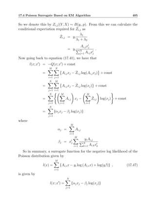


![412 A Review of Convexity in Optimization
However, it is important to remember that convex functions need not
always be continuous. To see this, consider the counter example given by the
function f :[0, 1] → R defined below.
f(x) =
1 if x = 0
x2
if x ∈ (0, 1]
Notice that f is a convex function defined on the convex set [0, 1] ⊂ R; how-
ever, f is not continuous at x = 0 since limx→0 f(x) = 0 6= 1. Furthermore, f
does not take on a local or global minimum because it never actually achieves
its infimum.
Of course, strict convexity is stronger than convexity, and in some cases,
it is very useful. However, the conditions required for strict convexity are a
bit different and are given below.
Property A.3. Basic properties of strictly convex functions - Let A be a convex
subset of RN
; let f : A → R be a strictly convex function; let g : A → R be
a convex function; let A be an N × M matrix of rank M; and let B be an
N × N symmetric and positive-definite matrix. Then the following are true.
a) h(x) = f(Ax) for x ∈ {x ∈ RM
: Ax ∈ A} is a strictly convex function.
b) h(x) = f(x) + g(x) for x ∈ A is a strictly convex function.
c) h(x) = ||x||2
B = xt
Bx for x ∈ A is a strictly convex function.
In some cases, it is useful to show that a function is convex by showing it
is the point-wise maximum of a set of functions.
Property A.4. Point-wise maximum over sets of convex functions - Let f1(x)
and f2(x) be two convex functions, and let g(x, y) be a convex function of x
for each value of y ∈ B where B is not necessarily a convex set. Then the
following are true.
a) h(x) = max{f1(x), f2(x)} is a convex function.
b) h(x) = supy∈B{g(x, y)} is a convex function.
When optimizing functions in high dimensional spaces, it is easy to be-
come trapped in local minima. For example, Figure A.1a illustrates a case in](https://image.slidesharecdn.com/s6hfi7xht12wwcizuy0v-mbip-book-230123055619-8f2fce45/85/MBIP-book-pdf-422-320.jpg)

![414 A Review of Convexity in Optimization
algorithms that we have seen operate locally on the function being minimized,
so without this theorem, these methods have little chance of obtaining a
global minimum for very complex functions.
However, while Theorem A.0.2 states that local and global minimum are
equivalent, it does not assure that they exist or that they are unique if they
do exist. The following theorem handles the issue of uniqueness when the
function being minimized is strictly convex.
Theorem A.0.3. Uniqueness of Global Minimum for a Strictly Convex Func-
tion
Let f :A → R be a strictly convex function on a convex set A ⊂ RN
. Then if
f has a global minimum at x∗
∈ A, then that global minimum must be unique
so that for all x ∈ A such that x 6= x∗
, we have that f(x) f(x∗
).
Existence of a global minimum is a more difficult matter. In fact, it is easy
to come up with examples of strictly convex functions which have no global
minimum. For example, the function f(x) = e−x
shown in Figure A.1(b) is
such an example. In this case, there is no global minimum because the func-
tion decreases monotonically toward infinity, never achieving its minimum
value.
In order to assure the existence of a global minimum, we will need some
additional concepts defined below.
Definition 32. Closed, Bounded, and Compact Sets
Let A ⊂ RN
, then we say that A is:
• Closed if every convergent sequence in A has its limit in A.
• Bounded if ∃M such that ∀x ∈ A , ||x|| M.
• Compact if A is both closed and bounded.
With these definitions, we can invoke a powerful theorem from analysis
which assures us that any continuous function takes on its minimum and
maximum on a compact set [71].
Theorem A.0.4. Weierstrass Extreme Value Theorem
Let f : A → R be a continuous function on a compact set A ⊂ RN
. Then
f takes on its global minimum in A, i.e., there exists an x∗
∈ A such that
∀x ∈ A , f(x∗
) ≤ f(x).
Putting together the Extreme Value Theorem with the results of Theo-](https://image.slidesharecdn.com/s6hfi7xht12wwcizuy0v-mbip-book-230123055619-8f2fce45/85/MBIP-book-pdf-424-320.jpg)


![417
to some unintended technical difficulties. So in order to guard against these
problems, mathematicians typically also assume that functions are proper,
closed, convex functions as a condition of theorems. The following two
definitions give meaning to these two terms.
Definition 36. Proper Functions
We say the function f : RN
→ R ∪ {∞} is proper if there exists an
x ∈ RN
so that f(x) ∞.
Definition 37. Closed Functions
We say the function f :RN
→ R ∪ {∞} is closed if for all α ∈ R, the
sublevel set Aα = {x ∈ RN
: f(x) ≤ α} is a closed set.
If a function is proper, then we know that it can be not infinite every-
where, which is typically a very reasonable assumption. Closure eliminates
the possibility that very strange things can happen when minimizing a convex
function. In particular, while it does not guarantee that a minimum exists,
it does removed certain pathological cases.
For example, consider the function
f(x) =
1t
x if ||x|| 1
∞ if ||x|| ≥ 1
,
where 1 is a column vector of 1′
s. Then in this case f is not closed since
{x ∈ RN
: f(x) ∞} is an open set. However, even though the function
is convex and tends to infinity as ||x|| → ∞, it does not take on a global or
local minimum. This is because the minimum “should” occur at x = −1,
but it doesn’t because f(−1) = ∞. Intuitively, the problem is that f is not
continuous at x = −1.
We conclude with a result that provides some additional intuition about
the nature of proper closed convex functions [5]. It states that, for a proper
convex function, closure is equivalent to lower semi-continuity, which is very
valuable when minimizing functions.
Theorem A.0.6. Continuity of Proper, Closed, Convex Functions
Let f :RN
→ R ∪ {∞} be a proper convex function. Then f is closed if and
only if it is lower semi-continuous.
Next we introduce the concept of a subgradient, which is very useful
when minimizing functions that are not continuously differentiable.](https://image.slidesharecdn.com/s6hfi7xht12wwcizuy0v-mbip-book-230123055619-8f2fce45/85/MBIP-book-pdf-427-320.jpg)


![422 Proximal Operator Theory
expansive functions is then non-expansive. (See problem 2).
Property B.1. Composition of Non-Expansive Functions - Let H : RN
→ RN
and Let F : RN
→ RN
be non-expansive functions. Then the composition of
the two functions, FH, is also non-expansive.
Moreover, as the name implies, the following property states that firmly
non-expansive mappings must always be non-expansive. (See problem 1)
Property B.2. Firmly Non-Expansive Implies Non-Expansive - Let H : RN
→
RN
be a firmly non-expansive function, then it is non-expansive.
Firmly non-expansive functions will be important to us for the following
reason. When H is firmly non-expansive, then the function, (2H − I), which
we will call the reflective resolvent1
is non-expansive. This is stated in the
following property proved in [4]. While this property may seem unmotivated
now, later we will see that it plays a central role in our analysis.
Property B.3. Firmly Non-Expansive Implies Non-Expansive Reflective Re-
solvent - Let H : RN
→ RN
be a firmly non-expansive function. Then the
reflective resolvent, R : RN
→ RN
where R = (2H − I), is non-expansive.
Next we introduce some important properties of proximal maps. To do
this, we will need to invoke the concepts of proper closed convex functions
explained in Appendix A and Definitions 36 and 37. The proper closed
conditions are typically assumed for convex functions taking values on the
extended real line, R ∪ {∞}, which we will sometimes refer to as extended
convex functions of Definition 35. The proper condition ensures that the
function can not be everywhere infinite, and Theorem A.0.6 ensures that
that a proper closed function is lower semi-continuous.
The following property, shown in [57], states that the proximal map of a
proper closed convex function is uniquely valued. This is important because
we know that for each input x ∈ RN
, there is a unique output, H(x) ∈ RN
.
1
This is not the true technical definition of the reflective resolvent used in monotone operator theory, but
we will adapt the definition for our somewhat simplified framework](https://image.slidesharecdn.com/s6hfi7xht12wwcizuy0v-mbip-book-230123055619-8f2fce45/85/MBIP-book-pdf-432-320.jpg)
![423
Property B.4. Proximal Maps of Proper Closed Convex Functions - Let h :
RN
→ R ∪ {∞} be a proper closed convex function, then its associated
proximal map given by
H(x) = arg min
v
h(v) +
1
2σ2
kx − vk2
,
for σ2
0 is a function H : RN
→ RN
.
In addition, the following property, shown in [57, p. 131], states that a the
proximal map of a proper closed convex function is firmly non-expansive.
Property B.5. Proximal Maps are Firmly Nonexpansive - Let H : RN
→ RN
be the proximal map of a proper closed convex function h : RN
→ R ∪ {∞}.
Then H is firmly non-expansive.
Putting together the results of Properties B.5 and B.3 yields a very im-
portant property of proximal maps for proper closed convex functions that
we will use throughout the chapter.
Property B.6. Reflective Resolvents of Proximal Maps
Let H : RN
→ RN
be the proximal map of a proper closed convex function
h : RN
→ R ∪ {∞}. Then its reflective resolvent, R = (2H − I) is non-
expansive.
In order to present Moreau’s Theorem [54, 72], we first introduce the
concept of a conservative function.
Definition 42. Conservative Functions
Let H : RN
→ RN
be a function. Then we say that H is a conservative
if their exists a function φ : RN
→ R such that ∀x ∈ RN
H(x) = ∇φ(x) .
Intuitively, a function is conservative if it is the gradient of some scalar
field. The classic example of a conservative vector field is from electromag-
netics in which the electric field is the gradient of the potential field. While
not all functions have this property, it turns out that there is a simple way
to determine if a function is conservative by using the following well known
theorem.](https://image.slidesharecdn.com/s6hfi7xht12wwcizuy0v-mbip-book-230123055619-8f2fce45/85/MBIP-book-pdf-433-320.jpg)
![424 Proximal Operator Theory
Theorem B.0.1. Conservation Theorem for Vector Fields
Let H : RN
→ RN
be a continuously differentiable function. Then H is
conservative if and only if for all x ∈ RN
,
∇H(x) = [∇H(x)]t
.
See for example [78, Theorem 2.6, p. 527] for proof.
Using these definitions, Moreau’s theorem can be stated in Chapter 10
as Theorem 10.2.1 [72, 54].
We conclude with some foundational material in the solution of fixed point
problems. Typically, when using proximal maps, we often need to compute
the fixed point of an operator T. A common way to do this is by using
the Mann iterations [13, 63] of equation (10.15). Below, we state the basic
theorem that we will use for this purpose.
Theorem B.0.2. Mann Iteration
Consider the iteration
w(k−1)
← (1 − ρ)w(k−1)
+ ρTw(k−1)
,
where ρ ∈ (0, 1), and T : RN
→ RN
.
• If T is non-expansive with a fixed point and ρ ∈ (0, 1) , then
limk→∞ w(k−1)
= w∗
where Tw∗
= w∗.
• If T is contractive and ρ ∈ (0, 1] , then limk→∞ w(k−1)
= w∗
where Tw∗
=
w∗.
We can use the results above to prove the convergence of the PnP-DR-
Serial Algorithm of Figure 10.8 when F and H are proximal maps. The
following theorem makes this precise.](https://image.slidesharecdn.com/s6hfi7xht12wwcizuy0v-mbip-book-230123055619-8f2fce45/85/MBIP-book-pdf-434-320.jpg)


![Appendix C
The Boltzmann and Gibbs
Distributions
In this appendix, we derive the general form of the discrete distribution known
as the Boltzmann or Gibbs distribution, and also derive some of its important
properties.
Let X be a discrete valued random variable with PMF given by px =
P{X = x}. In practice, X can be an array of discrete random variables, but
the key issue is that X takes on values in a discrete set. With each value or
state, x, we will associate an energy denoted by u(x). So then the expected
energy is given by
E = E[u(X)] =
X
x
u(x) px ,
and the entropy of the random variable X is then defined as
H = E[− log pX] =
X
x
−px log px .
The first law of thermodynamics states that energy is conserved for a
closed system. So the expected energy, E, must be constant. In addition,
the second law of thermodynamics states that the entropy of a closed system
can only increase with time. Therefore, a closed system in thermodynamic
equilibrium is one that has achieved its maximum entropy; so that no further
increases in entropy can occur and the system is in a stable equilibrium.
Therefore, the Boltzmann distribution can be derived by maximizing the
entropy, H, subject to the constraint that the energy is constant, i.e., E = Eo.
Based on this logic, we can derive the Boltzmann distribution by computing](https://image.slidesharecdn.com/s6hfi7xht12wwcizuy0v-mbip-book-230123055619-8f2fce45/85/MBIP-book-pdf-437-320.jpg)


![432 Proofs of Poisson Surrogates
Furthermore define the two functions
G1(x) =
Z x
0
g(t)dt
G2(x) =
Z xmin
x
g(t)dt .
Then we know that for x ∈ [xmin, 0]
G1(x) + G2(x) =
Z 0
xmin
g(t)dt = 0 .
Now if we can show that G1(x) ≥ 0 for all x ∈ [xmin, ∞), then we know
that
Q(x; x′
) − f(x) = G1(x) ≥ 0 , (D.1)
and we will have proved the result that Q is a surrogate for the minimization
of f(x). Furthermore, since Q(xmin; x′
)−f(xmin) = 0, then any smaller value
of the coefficient c′
c will violate the surrogate function relationship. So
therefore, if Q is a surrogate function for the minimization of f(x) then it
must be the tightest quadratic surrogate.
Next, we will show that g0 , g(xmin) ≥ 0. Since g(x) is a convex function
with g(xmin) = g0 and g(0) = 0, we know that g(t) ≤ g0
t
xmin
for all t ∈
[xmin, 0]. Therefore we have that
0 =
Z xmin
0
g(t)dt =
Z 0
xmin
g(t)dt ≤
Z 0
xmin
g0
t
xmin
dt =
g0
2
.
So therefore, we know that g0 ≥ 0. Now in order to prove the theorem, we
will consider two cases. Case 1 when g0 = 0 and case 2 when g0 0.
In case 1 when g0 = 0, then since g(t) is convex with g(0) = 0, then it
must be that g(t) ≤ 0 for t ∈ [xmin, 0). But since g(t) is continuous with
R 0
xmin
g(t)dt = 0, this implies that g(t) = 0 for t ∈ [xmin, 0), which implies
that for all x ∈ [xmin, 0]
G1(x) =
Z x
0
g(t)dt =
Z x
0
0 dt = 0 .
Also, since g(t) is convex and g(xmin) = g(0) = 0, it must be that g(x) ≥ 0
for all x ∈ [0, ∞), which implies that for all x ∈ [0, ∞]
G1(x) =
Z x
0
g(t)dt ≥ 0 .](https://image.slidesharecdn.com/s6hfi7xht12wwcizuy0v-mbip-book-230123055619-8f2fce45/85/MBIP-book-pdf-442-320.jpg)
![433
So for case 1 we have the result that G1(x) ≥ 0 for all x ∈ [xmin, ∞).
In case 2, we assume g0 0. Since the function g(t) is continuous with
R 0
xmin
g(t)dt = 0, there must exist a point x1 ∈ (xmin, 0) such that g(x1) 0.
Therefore, by the intermediate value theorem, there must exist a point x0 ∈
(xmin, x1) such that g(x0) = 0.
Since g(t) is convex, then the following results must hold.
R1 g(x) ≥ 0 for all x ∈ [xmin, x0]
R2 g(x) ≤ 0 for all x ∈ [x0, 0]
R3 g(x) ≥ 0 for all x ∈ [0, ∞)
Now result R3 implies that for all x ∈ [0, ∞]
G1(x) =
Z x
0
g(t)dt ≥ 0 .
Result R2 implies that for all x ∈ [x0, 0]
G1(x) =
Z x
0
g(t)dt = −
Z 0
x
g(t)dt ≥ 0 .
Result R1 implies that for all x ∈ [xmin, x0]
G1(x) = −G2(x) = −
Z xmin
x
g(t)dt =
Z x
xmin
g(t)dt ≥ 0 .
So for case 2 we have again shown the result that G1(x) ≥ 0 for all x ∈
[xmin, ∞).
The following is a proof of Theorem 17.3.2 from Chapter 17.
Proof. In order to simplify the notation of the proof, we may with out loss
of generality assume that x′
= 0 and f(x′
) = 0. In this case, it must then
be that xmin 0 and b = 0. Also, since f(x) is convex and f′
(x) is concave
both must also be continuous functions of [xmin, ∞).
Now in this case, Q(0; 0) = f(0) = 0, so in order to show that Q is
a surrogate for the minimization of f(x), we need only show that for all](https://image.slidesharecdn.com/s6hfi7xht12wwcizuy0v-mbip-book-230123055619-8f2fce45/85/MBIP-book-pdf-443-320.jpg)
![434 Proofs of Poisson Surrogates
x ∈ [xmin, ∞) that Q(x; 0) ≥ f(x). To do this, we start by defining the
convex function g(t) = ct − f′
(t). Then we can show that
Q(x; x′
) − f(x) =
c
2
x2
−
Z x
0
f′
(t)dt
=
Z x
0
(ct − f′
(t)) dt
=
Z x
0
g(t)dt .
Furthermore if we define the function
G1(x) =
Z x
0
g(t)dt ,
then if we can show that G1(x) ≥ 0 for all x ∈ [xmin, ∞), then we know that
Q(x; x′
) − f(x) = G1(x) ≥ 0 , (D.2)
and we have proved the result that Q is a surrogate for the minimization of
f(x).
By the specific choice of c from equation (17.21), it is easily show that
g(xmin) = 0. Therefore, since g(t) is convex and g(0) = 0, we know that the
following results must hold.
R1 g(x) ≤ 0 for all x ∈ [xmin, 0]
R2 g(x) ≥ 0 for all x ∈ [0, ∞)
Now result R2 implies that for all x ∈ [0, ∞]
G1(x) =
Z x
0
g(t)dt ≥ 0 .
Result R1 implies that for all x ∈ [xmin, 0]
G1(x) =
Z x
0
g(t)dt = −
Z 0
x
g(t)dt ≥ 0 .
So we have shown the result that G1(x) ≥ 0 for all x ∈ [xmin, ∞).](https://image.slidesharecdn.com/s6hfi7xht12wwcizuy0v-mbip-book-230123055619-8f2fce45/85/MBIP-book-pdf-444-320.jpg)
![Appendix E
Book Notation
General Notation:
1. Reals - R
2. Integers - Z
3. Non-negative Reals - R+
4. N dimensional Non-negative Reals - R+N
5. Non-negative Integers - Z+
6. Gradient is a column vector!
7. Vector norm ||x||
8. Definition ,
9. Expectation E[X]
10. Expectation Eθ[X]
11. Variance Var[X]
12. Circular convolution xn ⊛ hn
13. Column vector of 1’s, 1.
14. Column vector of 0’s, 0.
15. Approximately equal x ≈ y](https://image.slidesharecdn.com/s6hfi7xht12wwcizuy0v-mbip-book-230123055619-8f2fce45/85/MBIP-book-pdf-445-320.jpg)
![436 Book Notation
16. Interior of set int(S)
17. clip{x, [a, b]} - clips the value x to the interval [a, b]
18. clip{x, Ω} - projects the vector x onto the convex set Ω.
19. clip
x, R+N
- enforce positivity constraint on x.
20. const - additive constant
21. 0 - null vector
Probability (Chapter 2):
• Y or X ∈ Rp
- multivariate Gaussian observations
• X1, · · · , Xn - i.i.d. samples from a distribution
• P(A) - Probability of an event A ⊂ Ω
• P{X ≤ t} - Probability of the event A = {ω ∈ Ω : X(ω) ≤ t}
• P
X
1+Y ≤ t - Probability of the event A =
n
ω ∈ Ω : X(ω)
1+Y (ω) ≤ t
o
Gaussian prior models (Chapters 3 and 4):
• n ∈ [1, · · · , N] - 1-D index set
• s = (s1, s2) ∈ [1, · · · , N]2
- 2-D index set with s1 being the row and s2
being the column.
• s ∈ S - arbitrary index set
• N = |S| - number of elements in lattice
• Xn - random process in 1 or more dimensions
• Es - causal or non-causal prediction error
• Causal notation
– H - causal predictor matrix
– A = I − H - causal predictor matrix
– E = AX = (I − H)X - causal prediction error](https://image.slidesharecdn.com/s6hfi7xht12wwcizuy0v-mbip-book-230123055619-8f2fce45/85/MBIP-book-pdf-446-320.jpg)


![439
• Rp
- observation space
• Yn ∈ Rp
for n = 1, · · · , N - observed data and associated space
• Xn ∈ Ω with |Ω| = M - unobserved data and associated space
• θ(k)
- result of kth
EM iteration
• Nm, bm, Rm - sufficient statistics for each class
• N̄m, b̄m, R̄m - expected sufficient statistics for each class
• p - dimension of observation vector
• θ, θ̃ - new and old parameters respectively
• πm, µm, σ2
m - parameters for mth
mixture component
• θ = [π0, µ0, σ2
0, · · · , πM−1, µM−1, σ2
M−1] - full parameter vector
Markov Chain and HMM (Chapter 13):
• Xn - discrete time Markov chain
• 0 ≤ n ≤ N with X0 being the initial state
• π
(n)
j = P{Xn = j} - state distribution at time n
• P
(n)
i,j - nonhomogeneous state transition probability
• τj = π
(0)
j - initial state distribution
• Nj = δ(X0 − j) - initial state statistics
• Kj =
PN
n=1 δ(Xn − j) =
PM−1
i=0 Ki,j - state membership statistics
• Ki,j =
PN
n=1 δ(Xn − j)δ(Xn−1 − i) - state transition statistics
• bj =
PN−1
n=0 ynδ(xn − j) - first order class statistics
• Sj =
PN−1
n=0 ynyt
nδ(xn − j) - second order class statistics
• Ω = [0, · · · , M − 1] - set of discrete states
• θ = [τj, Pi,j : for i, j ∈ Ω] - parameter vector](https://image.slidesharecdn.com/s6hfi7xht12wwcizuy0v-mbip-book-230123055619-8f2fce45/85/MBIP-book-pdf-449-320.jpg)


![Bibliography
[1] S. Alliney and S. A. Ruzinsky. An algorithm for the minimization of mixed l1 and l2 norms
with application to Bayesian estimation. IEEE Trans. on Signal Processing, 42(3):618–627,
March 1994.
[2] L. Baum, T. Petrie, G. Soules, and N. Weiss. A maximization technique occurring in the statis-
tical analysis of probabilistic functions of Markov chains. Ann. Math. Statistics, 41(1):164–171,
1970.
[3] L. E. Baum and T. Petrie. Statistical inference for probabilistic functions of finite state Markov
chains. Ann. Math. Statistics, 37:1554–1563, 1966.
[4] H. H. Bauschke, S. M. Moffat, and X. Wang. Firmly nonexpansive mappings and maxi-
mally monotone operators: Correspondence and duality. Set-Valued and Variational Analysis,
20:131153, 2012.
[5] D. P. Bertsekas. Convex Analysis and Optimization. Athena Scientific, 2003.
[6] D. P. Bertsekas and J. N. Tsitsiklis. Parallel and Distributed Computation: Numerical Methods.
Prentice-Hall, 1989.
[7] J. Besag. Spatial interaction and the statistical analysis of lattice systems. Journal of the
Royal Statistical Society B, 36(2):192–236, 1974.
[8] J. Besag. Efficiency of pseudolikelihood estimation for simple Gaussian fields. Biometrica,
64(3):616–618, 1977.
[9] J. Besag. On the statistical analysis of dirty pictures. Journal of the Royal Statistical Society
B, 48(3):259–302, 1986.
[10] J. Besag. Towards Bayesian image analysis. Journal of Applied Statistics, 16(3):395–407, 1989.
[11] A. Blake. Comparison of the efficiency of deterministic and stochastic algorithms for visual re-
construction. IEEE Trans. on Pattern Analysis and Machine Intelligence, 11(1):2–30, January
1989.
[12] A. Blake and A. Zisserman. Visual Reconstruction. MIT Press, Cambridge, Massachusetts,
1987.
[13] J. Borwein, S. Reich, and I. Shafrir. Krasnoselski-mann iterations in normed spaces. Canad.
Math. Bull., 35(1):21–28, 1992.](https://image.slidesharecdn.com/s6hfi7xht12wwcizuy0v-mbip-book-230123055619-8f2fce45/85/MBIP-book-pdf-455-320.jpg)
![446 BIBLIOGRAPHY
[14] C. A. Bouman and B. Liu. Multiple resolution segmentation of textured images. IEEE Trans.
on Pattern Analysis and Machine Intelligence, 13(2):99–113, February 1991.
[15] C. A. Bouman and K. Sauer. A generalized Gaussian image model for edge-preserving MAP
estimation. IEEE Trans. on Image Processing, 2(3):296–310, July 1993.
[16] S. Boyd, N. Parikh, E. Chu, B. Peleato, and J. Eckstein. Distributed optimization and statisti-
cal learning via the alternating direction method of multipliers. Found. Trends Mach. Learn.,
3(1):1–122, Jan. 2011.
[17] S. Boyd and L. Vandenberghe. Convex Optimization. Cambridge University Press, Cambridge
UK, 2009.
[18] Y. Boykov and V. Kolmogorov. An experimental comparison of min-cut/max-flow algorithms
for energy minimization in vision. IEEE Trans. on Pattern Analysis and Machine Intelligence,
26(9):1124–1137, 2004.
[19] G. T. Buzzard, S. H. Chan, S. Sreehari, and C. A. Bouman. Plug-and-play unplugged:
Optimization-free reconstruction using consensus equilibrium. SIAM J. Imaging Sciences,
11(3):2001–2020, Dec. 2018.
[20] M. L. Comer and E. J. Delp. The em/mpm algorithm for segmentation of textured images:
Analysis and further experimental results. IEEE Trans. on Image Processing, 9(10):1731–1744,
October 2000.
[21] H. Derin, H. Elliott, R. Cristi, and D. Geman. Bayes smoothing algorithms for segmentation
of binary images modeled by Markov random fields. IEEE Trans. on Pattern Analysis and
Machine Intelligence, PAMI-6(6):707–719, November 1984.
[22] J. Douglas and H. H. R. Jr. On the numerical solution of heat conduction problems in two
and three space variables. Trans. of the American Mathematical Society, 82(2):421439, 1956.
[23] J. Eckstein. Augmented lagrangian and alternating directions methods for convex optimiza-
tion: A tutorial and some illustrative computational results. Technical Report RRR 32-2012,
RUTCOR Rutgers Center for Operations Research, Rutger University, Rutger University, De-
cember 2012.
[24] J. Eckstein and D. P. Bertsekas. On the Douglas-Rachford splitting method and the proximal
point algorithm for maximal monotone operators. Mathematical Programming, 55(1-3):293–
318, 1992.
[25] H. Feng, W. C. Karl, and D. A. Castanon. A curve evolution approach to object-based
tomographic reconstruction. IEEE Trans. on Image Processing, 12(1):44–57, March 2003.
[26] J. Fessler, E. Ficaro, N. Clinthorne, and K. Lange. Grouped-coordinate ascent algorithms for
penalized-likelihood transmi ssion image reconstruction. IEEE Trans. on Medical Imaging,
16(2):166–175, April 1997.
[27] L. R. Ford and D. R. Fulkerson. Flows in Networks. Princeton University Press, Princeton,
NJ, 1962.
[28] M. Fortin and R. Glowinski. On Decomposition-coordination methods using an augmented
Lagrangian. North-Holland: Amsterdam, 1983.](https://image.slidesharecdn.com/s6hfi7xht12wwcizuy0v-mbip-book-230123055619-8f2fce45/85/MBIP-book-pdf-456-320.jpg)
![BIBLIOGRAPHY 447
[29] T. Frese, C. A. Bouman, and K. Sauer. Multiscale Bayesian methods for discrete tomography.
In G. T. Herman and A. Kuba, editors, Discrete Tomography: Foundations, Algorithms and
Applications, pages 237–261. Birkhauser Boston, Cambridge, MA, 1999.
[30] D. Gabay. Applications of the Method of Multipliers to Variational Inequalities. North-Holland:
Amsterdam, 1983.
[31] D. Geman and G. Reynolds. Constrained restoration and the recovery of discontinuities. IEEE
Trans. on Pattern Analysis and Machine Intelligence, 14(3):367–383, March 1992.
[32] D. Geman and C. Yang. Nonlinear image recovery with half-quadratic regularization. IEEE
Trans. Image Processing, 4(7):932–946, 1975.
[33] S. Geman and D. Geman. Stochastic relaxation, Gibbs distributions and the Bayesian restora-
tion of images. IEEE Trans. on Pattern Analysis and Machine Intelligence, PAMI-6:721–741,
November 1984.
[34] S. Geman and C. Graffigne. Markov random field image models and their applications to
computer vision. In Proc. of the Intl Congress of Mathematicians, pages 1496–1517, Berkeley,
CA, 1986.
[35] S. Geman and D. McClure. Bayesian images analysis: An application to single photon emission
tomography. In Proc. Statist. Comput. sect. Amer. Stat. Assoc., pages 12–18, Washington,
DC, 1985.
[36] S. Geman and D. McClure. Statistical methods for tomographic image reconstruction. Bull.
Int. Stat. Inst., LII-4:5–21, 1987.
[37] P. J. Green. Bayesian reconstruction from emission tomography data using a modified EM
algorithm. IEEE Trans. on Medical Imaging, 9(1):84–93, March 1990.
[38] P. J. Green and X. liang Han. Metropolis methods, Gaussian proposals and antithetic variables.
In P. Barone, A. Frigessi, and M. Piccioni, editors, Stochastic Models, Statistical methods, and
Algorithms in Image Analysis, pages 142–164. Springer-Verlag, Berlin, 1992.
[39] D. Greig, B. Porteous, and A. Seheult. Exact maximum a posteriori estimation for binary
images. J. R. Statist. Soc. B, 51(2):271–278, 1989.
[40] W. K. Hastings. Monte Carlo sampling methods using Markov chains and their applications.
Biometrika, 57(1):97–109, 1970.
[41] T. Hebert and R. Leahy. A generalized EM algorithm for 3-D Bayesian reconstruction from
Poisson data using Gibbs priors. IEEE Trans. on Medical Imaging, 8(2):194–202, June 1989.
[42] M. R. Hestenes. Multiplier and gradient methods. Journal of Optimization Theory and Ap-
plications, 4(5):303–320, 1969.
[43] P. J. Huber. Robust Statistics. Wiley, New York, 1981.
[44] E. Ising. Beitrag zur theorie des ferromagnetismus. Z. Phys., 31:253258, 1925.
[45] L. Kantorovich and G. Akilov. Functional Analysis in Normed Spaces. Fitzmatgiz, Moscow,
1959.](https://image.slidesharecdn.com/s6hfi7xht12wwcizuy0v-mbip-book-230123055619-8f2fce45/85/MBIP-book-pdf-457-320.jpg)
![448 BIBLIOGRAPHY
[46] Z. Kato, M. Berthod, and J. Zerubia. Parallel image classification using multiscale Markov
random fields. In Proc. of IEEE Int’l Conf. on Acoust., Speech and Sig. Proc., volume 5, pages
137–140, Minneapolis, MN, April 27-30 1993.
[47] R. Kindermann and J. Snell. Markov Random Fields and their Applications. American Math-
ematical Society, Providence, 1980.
[48] W. Lenz. Beitrage zum verstandnis der magnetischen eigenschaften in festen korpern.
Physikalische Zeitschrift, page 613615, 1921.
[49] D. G. Luenberger. Linear and Nonlinear Programming. Addison-Wesley Publishing Company,
Reading Massachusetts, 1989.
[50] S. Majee, T. Balke, C. A. J. Kemp, G. T. Buzzard, and C. A. Bouman. 4d x-ray ct reconstruc-
tion using multi-slice fusion. In 2019 IEEE Int. Conference on Computational Photography
(ICCP), pages 1–8, Tokyo, Japan, May 2019.
[51] J. Marroquin, S. Mitter, and T. Poggio. Probabilistic solution of ill-posed problems in com-
putational vision. Journal of the American Statistical Association, 82:76–89, March 1987.
[52] N. Metropolis, A. Rosenbluth, M. Rosenbluth, A. Teller, and E. Teller. Equations of state
calculations by fast computing machines. J. Chem. Phys., 21:1087–1091, 1953.
[53] A. Mohammad-Djafari. Joint estimation of parameters and hyperparameters in a Bayesian
approach of solving inverse problems. In Proc. of IEEE Int’l Conf. on Image Proc., volume II,
pages 473–476, Lausanne, Switzerland, September 16-19 1996.
[54] J.-J. Moreau. Proximité et dualité dans un espace hilbertien. Bulletin de la Société
mathématique de France, 93:273–299, 1965.
[55] L. Onsager. Crystal statistics i. a two-dimensional model. Physical Review Letters, 65:117–149,
1944.
[56] J. M. Ortega and W. C. Rheinoboldt. Iterative Solutions of Nonlinear Equations in Several
Variables, pages 253–255. Academic, New York, 1970.
[57] N. Parikh and S. Boyd. Proximal algorithms. Found. Trends Optim., 1(3):127239, Jan 2014.
[58] R. E. Peierls. Statistical theory of adsorption with interaction between the adsorbed atoms.
Proc. Camb. Phil. Soc., 32:471–476, 1936.
[59] P. H. Peskun. Optimum Monte-Carlo sampling using Markov chains. Biometrika, 60(3):607–
612, 1973.
[60] A. R. D. Pierro. A modified expectation maximization algorithm for penalized likelihood
estimation in emission tomography. IEEE Trans. Med. Imaging, 14(1):132–137, 1995.
[61] M. J. D. Powell. A Method for Nonlinear Constraints in Minimization Problems, pages 283–
298. Academic Press, New York, 1969.
[62] E. Redner and H. Walker. Mixture densities, maximum likelihood and the EM algorithm.
SIAM Review, 26(2), April 1984.](https://image.slidesharecdn.com/s6hfi7xht12wwcizuy0v-mbip-book-230123055619-8f2fce45/85/MBIP-book-pdf-458-320.jpg)
![BIBLIOGRAPHY 449
[63] S. Reich and A. J. Zaslavski. Convergence of krasnoselskii-mann iterations of nonexpansive
operators. Mathematical and Computer Modelling., 32:1423–1431, 2000.
[64] S. M. Ross. Stochastic Processes. John Wiley Sons, New York, 1983.
[65] L. Rudin, S. Oscher, and E. Fatemi. Nonlinear total variation based noise removal algorithms.
Phys. D, 60:259–268, November 1992.
[66] K. Sauer and C. Bouman. Bayesian estimation of transmission tomograms using segmentation
based optimization. IEEE Trans. on Nuclear Science, 39:1144–1152, 1992.
[67] K. Sauer and C. A. Bouman. A local update strategy for iterative reconstruction from pro-
jections. IEEE Trans. on Signal Processing, 41(2):534–548, February 1993.
[68] L. Shepp and Y. Vardi. Maximum likelihood reconstruction for emission tomography. IEEE
Trans. on Medical Imaging, MI-1(2):113–122, October 1982.
[69] S. Silvey. Statistical Inference. Chapman and Hall, London, 1975.
[70] M. Slater. Lagrange multipliers revisisted. Technical Report 80, Cowles Foundation for Re-
search in Economics, Yale University, November 1950.
[71] H. Sohrab. Basic Real Analysis. Springer New York, 2014.
[72] S. Sreehari, B. W. S. V. Venkatakrishnan, L. F. D. Gregery T. Buzzard, J. P. Simmons,
and C. A. Bouman. Plug-and-play priors for bright field electron tomography and sparse
interpolation. 2(4):408–423, Sept. 2016.
[73] R. Stevenson and E. Delp. Fitting curves with discontinuities. Proc. of the first international
workshop on robust computer vision, pages 127–136, October 1-3 1990.
[74] J.-B. Thibault, K. Sauer, C. Bouman, and J. Hsieh. A three-dimensional statistical approach to
improved image quality for multi-slice helical ct. Medical Physics, 34(11):4526–4544, November
2007.
[75] R. Tibshirani. Regression shrinkage and selection via the lasso. Journal of the Royal Statistical
Society. Series B, 58(1):267288, 1996.
[76] A. Tikhonov and V. Arsenin. Solutions of Ill-Posed Problems. Winston and Sons, New York,
1977.
[77] S. V. Venkatakrishanan, C. A. Bouman, and B. Wohlberg. Plug-and-play priors for model
based reconstruction. In IEEE 2013 IEEE Global Conference on Signal and Information
Processing (GlobalSIP), pages 945–948, Austin, TX, December 3-5 2013.
[78] R. E. Williamson, R. H. Crowell, and H. F. Trotter. Calculus of vector functions. Prentice-Hall,
1972.
[79] E. Wong and B. Hajek. Stochastic Processes in Engineering Systems. Springer Texts in
Electrical Engineering. Springer New York Inc., 1985.
[80] J. Woods, S. Dravida, and R. Mediavilla. Image estimation using double stochastic Gaussian
random field models. IEEE Trans. on Pattern Analysis and Machine Intelligence, PAMI-
9(2):245–253, March 1987.](https://image.slidesharecdn.com/s6hfi7xht12wwcizuy0v-mbip-book-230123055619-8f2fce45/85/MBIP-book-pdf-459-320.jpg)
![450 BIBLIOGRAPHY
[81] C. Wu. On the convergence properties of the EM algorithm. Annals of Statistics, 11(1):95–103,
1983.
[82] Z. Yu, J.-B. Thibault, C. A. Bouman, K. D. Sauer, and J. Hsieh. Fast model-based x-ray
ct reconstruction using spatially nonhomogeneous icd optimization. IEEE Trans. on Image
Processing, 20(1):161–175, 2011.
[83] J. Zheng, S. S. Saquib, K. Sauer, and C. A. Bouman. Parallelizable Bayesian tomography
algorithms with rapid, guaranteed convergence. IEEE Trans. on Image Processing, 9(10):1745–
1759, Oct. 2000.](https://image.slidesharecdn.com/s6hfi7xht12wwcizuy0v-mbip-book-230123055619-8f2fce45/85/MBIP-book-pdf-460-320.jpg)