The document summarizes Approximate Bayesian Computation (ABC). It discusses how ABC provides a way to approximate Bayesian inference when the likelihood function is intractable or too computationally expensive to evaluate directly. ABC works by simulating data under different parameter values and accepting simulations that are close to the observed data according to a distance measure and tolerance level. Key points discussed include: - ABC provides an approximation to the posterior distribution by sampling from simulations that fall within a tolerance of the observed data. - Summary statistics are often used to reduce the dimension of the data and improve the signal-to-noise ratio when applying the tolerance criterion. - Random forests can help select informative summary statistics and provide semi-automated ABC

1. Approximate Bayesian computation
Christian P. Robert
U. Paris Dauphine PSL & Warwick U. & CREST ENSAE
Laplace’s Demon, 13 May, 2020

2. Not to be confused with...
The XKCD of ABC
Christian P. Robert
(Paris Dauphine PSL & Warwick U.)
JSM 2019, Denver, Colorado

3. Co-authors
Jean-Marie Cornuet, Arnaud Estoup (INRA Montpellier)
David Frazier, Gael Martin (Monash U)
Jean-Michel Marin (U Montpellier)
Kerrie Mengersen (QUT)
Espen Bernton, Pierre Jacob, Natesh Pillai (Harvard U)
Judith Rousseau (U Oxford)
Gr´egoire Clart´e, Robin Ryder, Julien Stoehr (U Paris
Dauphine)

4. Outline
1 Motivation
2 Concept
3 Implementation
4 Big data issues
5 big parameter issues
6 ABC postdoc positions

5. another webinar

6. Posterior distribution
Central concept of Bayesian inference:
π( θ
parameter
| xobs
observation
)
proportional
∝ π(θ)
prior
× L(θ | xobs
)
likelihood
Drives
derivation of optimal decisions
assessment of uncertainty
model selection
prediction
[McElreath, 2015]

7. Monte Carlo representation
Exploration of Bayesian posterior π(θ|xobs) may (!) require to
produce sample
θ1, . . . , θT
distributed from π(θ|xobs) (or asymptotically by Markov chain
Monte Carlo aka MCMC)
[McElreath, 2015]

8. Difficulties
MCMC = workhorse of practical Bayesian analysis (BUGS,
JAGS, Stan, &tc.), except when product
π(θ) × L(θ | xobs
)
well-defined but numerically unavailable or too costly to
compute
Only partial solutions are available:
demarginalisation (latent variables)
exchange algorithm (auxiliary variables)
pseudo-marginal (unbiased estimator)

9. Difficulties
MCMC = workhorse of practical Bayesian analysis (BUGS,
JAGS, Stan, &tc.), except when product
π(θ) × L(θ | xobs
)
well-defined but numerically unavailable or too costly to
compute
Only partial solutions are available:
demarginalisation (latent variables)
exchange algorithm (auxiliary variables)
pseudo-marginal (unbiased estimator)

10. Example 1: Dynamic mixture
Mixture model
{1 − wµ,τ(x)}fβ,λ(x) + wµ,τ(x)gε,σ(x) x > 0
where
fβ,λ Weibull density,
gε,σ generalised Pareto density, and
wµ,τ Cauchy (arctan) cdf
Intractable normalising constant
C(µ, τ, β, λ, ε, σ) =
∞
0
{(1 − wµ,τ(x))fβ,λ(x) + wµ,τ(x)gε,σ(x)} dx
[Frigessi, Haug & Rue, 2002]

11. Example 2: truncated Normal
Given set A ⊂ Rk (k large), truncated Normal model
f(x | µ, Σ, A) ∝ exp{−(x − µ)T
Σ−1
(x − µ)/2} IA(x)
with intractable normalising constant
C(µ, Σ, A) =
A
exp{−(x − µ)T
Σ−1
(x − µ)/2}dx

12. Example 3: robust Normal statistics
Normal sample
x1, . . . , xn ∼ N(µ, σ2
)
summarised into (insufficient)
^µn = med(x1, . . . , xn)
and
^σn = mad(x1, . . . , xn)
= med |xi − ^µn|
Under a conjugate prior π(µ, σ2), posterior close to intractable.
but simulation of (^µn, ^σn) straightforward

13. Example 3: robust Normal statistics
Normal sample
x1, . . . , xn ∼ N(µ, σ2
)
summarised into (insufficient)
^µn = med(x1, . . . , xn)
and
^σn = mad(x1, . . . , xn)
= med |xi − ^µn|
Under a conjugate prior π(µ, σ2), posterior close to intractable.
but simulation of (^µn, ^σn) straightforward

14. Example 4: exponential random graph
ERGM: binary random vector x indexed
by all edges on set of nodes plus graph
f(x | θ) =
1
C(θ)
exp(θT
S(x))
with S(x) vector of statistics and C(θ)
intractable normalising constant
[Grelaud & al., 2009; Everitt, 2012; Bouranis & al., 2017]

15. Realistic[er] applications
Kingman’s coalescent in population genetics
[Tavar´e et al., 1997; Beaumont et al., 2003]
α-stable distributions
[Peters et al, 2012]
complex networks
[Dutta et al., 2018]
astrostatistics & cosmostatistics
[Cameron & Pettitt, 2012; Ishida et al., 2015]

16. Concept
2 Concept
algorithm
summary statistics
random forests
calibration of tolerance
3 Implementation
4 Big data issues
5 big parameter issues
6 ABC postdoc positions

17. A?B?C?
A stands for approximate [wrong
likelihood]
B stands for Bayesian [right prior]
C stands for computation
[producing a parameter sample]

18. A?B?C?
Rough version of the data [from dot
to ball]
Non-parametric approximation of
the likelihood [near actual
observation]
Use of non-sufficient statistics
[dimension reduction]
Monte Carlo error [and no
unbiasedness]

19. A seemingly na¨ıve representation
When likelihood f(x|θ) not in closed form, likelihood-free
rejection technique:
ABC-AR algorithm
For an observation xobs ∼ f(x|θ), under the prior π(θ), keep
jointly simulating
θ ∼ π(θ) , z ∼ f(z|θ ) ,
until the auxiliary variable z is equal to the observed value,
z = xobs
[Diggle & Gratton, 1984; Rubin, 1984; Tavar´e et al., 1997]

20. A seemingly na¨ıve representation
When likelihood f(x|θ) not in closed form, likelihood-free
rejection technique:
ABC-AR algorithm
For an observation xobs ∼ f(x|θ), under the prior π(θ), keep
jointly simulating
θ ∼ π(θ) , z ∼ f(z|θ ) ,
until the auxiliary variable z is equal to the observed value,
z = xobs
[Diggle & Gratton, 1984; Rubin, 1984; Tavar´e et al., 1997]

21. Why does it work?
The mathematical proof is trivial:
f(θi) ∝
z∈D
π(θi)f(z|θi)Iy(z)
∝ π(θi)f(y|θi)
= π(θi|y)
[Accept–Reject 101]
But very impractical when
Pθ(Z = xobs
) ≈ 0

22. Why does it work?
The mathematical proof is trivial:
f(θi) ∝
z∈D
π(θi)f(z|θi)Iy(z)
∝ π(θi)f(y|θi)
= π(θi|y)
[Accept–Reject 101]
But very impractical when
Pθ(Z = xobs
) ≈ 0

23. A as approximative
When y is a continuous random variable, strict equality
z = xobs
is replaced with a tolerance zone
ρ(xobs
, z) ≤ ε
where ρ is a distance
Output distributed from
π(θ) Pθ{ρ(xobs
, z) < ε}
def
∝ π(θ|ρ(xobs
, z) < ε)
[Pritchard et al., 1999]

24. A as approximative
When y is a continuous random variable, strict equality
z = xobs
is replaced with a tolerance zone
ρ(xobs
, z) ≤ ε
where ρ is a distance
Output distributed from
π(θ) Pθ{ρ(xobs
, z) < ε}
def
∝ π(θ|ρ(xobs
, z) < ε)
[Pritchard et al., 1999]

25. ABC algorithm
Algorithm 1 Likelihood-free rejection sampler
for i = 1 to N do
repeat
generate θ from prior π(·)
generate z from sampling density f(·|θ )
until ρ{η(z), η(xobs)} ≤ ε
set θi = θ
end for
where η(xobs) defines a (not necessarily sufficient) statistic
Custom: η(xobs) called summary statistic

26. ABC algorithm
Algorithm 2 Likelihood-free rejection sampler
for i = 1 to N do
repeat
generate θ from prior π(·)
generate z from sampling density f(·|θ )
until ρ{η(z), η(xobs)} ≤ ε
set θi = θ
end for
where η(xobs) defines a (not necessarily sufficient) statistic
Custom: η(xobs) called summary statistic

27. Example 3: robust Normal statistics
mu=rnorm(N<-1e6) #prior
sig=sqrt(rgamma(N,2,2))
medobs=median(obs)
madobs=mad(obs) #summary
for(t in diz<-1:N){
psud=rnorm(1e2)/sig[t]+mu[t]
medpsu=median(psud)-medobs
madpsu=mad(psud)-madobs
diz[t]=medpsuˆ2+madpsuˆ2}
#ABC subsample
subz=which(diz<quantile(diz,.1))

28. Exact ABC posterior
Algorithm samples from marginal in z of [exact] posterior
πABC
ε (θ, z|xobs
) =
π(θ)f(z|θ)IAε,xobs
(z)
Aε,xobs ×Θ π(θ)f(z|θ)dzdθ
,
where Aε,xobs = {z ∈ D|ρ{η(z), η(xobs)} < ε}.
Intuition that proper summary statistics coupled with small
tolerance ε = εη should provide good approximation of the
posterior distribution:
πABC
ε (θ|xobs
) = πABC
ε (θ, z|xobs
)dz ≈ π{θ|η(xobs
)}

29. Exact ABC posterior
Algorithm samples from marginal in z of [exact] posterior
πABC
ε (θ, z|xobs
) =
π(θ)f(z|θ)IAε,xobs
(z)
Aε,xobs ×Θ π(θ)f(z|θ)dzdθ
,
where Aε,xobs = {z ∈ D|ρ{η(z), η(xobs)} < ε}.
Intuition that proper summary statistics coupled with small
tolerance ε = εη should provide good approximation of the
posterior distribution:
πABC
ε (θ|xobs
) = πABC
ε (θ, z|xobs
)dz ≈ π{θ|η(xobs
)}

30. Why summaries?
reduction of dimension
improvement of signal to noise ratio
reduce tolerance ε considerably
whole data may be unavailable (as in Example 3)
medobs=median(obs)
madobs=mad(obs) #summary

31. Example 6: MA inference
Moving average model MA(2):
xt = εt + θ1εt−1 + θ2εt−2 εt
iid
∼ N(0, 1)
Comparison of raw series:

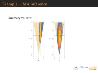
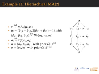
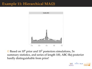
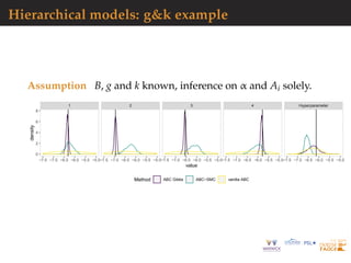
32. Example 6: MA inference
Moving average model MA(2):
xt = εt + θ1εt−1 + θ2εt−2 εt
iid
∼ N(0, 1)
[Feller, 1970]
Comparison of acf’s:

33. Example 6: MA inference
Summary vs. raw:

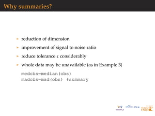
34. Why not summaries?
loss of sufficient information when πABC(θ|xobs) replaced
with πABC(θ|η(xobs))
arbitrariness of summaries
uncalibrated approximation
whole data may be available (at same cost as summaries)
(empirical) distributions may be compared (Wasserstein
distances)
[Bernton et al., 2019]

35. Summary selection strategies
Fundamental difficulty of selecting summary statistics when
there is no non-trivial sufficient statistic [except when done by
experimenters from the field]

36. Summary selection strategies
Fundamental difficulty of selecting summary statistics when
there is no non-trivial sufficient statistic [except when done by
experimenters from the field]
1. Starting from large collection of summary statistics, Joyce
and Marjoram (2008) consider the sequential inclusion into the
ABC target, with a stopping rule based on a likelihood ratio test

37. Summary selection strategies
Fundamental difficulty of selecting summary statistics when
there is no non-trivial sufficient statistic [except when done by
experimenters from the field]
2. Based on decision-theoretic principles, Fearnhead and
Prangle (2012) end up with E[θ|xobs] as the optimal summary
statistic

38. Summary selection strategies
Fundamental difficulty of selecting summary statistics when
there is no non-trivial sufficient statistic [except when done by
experimenters from the field]
3. Use of indirect inference by Drovandi, Pettit, & Paddy (2011)
with estimators of parameters of auxiliary model as summary
statistics

39. Summary selection strategies
Fundamental difficulty of selecting summary statistics when
there is no non-trivial sufficient statistic [except when done by
experimenters from the field]
4. Starting from large collection of summary statistics, Raynal
& al. (2018, 2019) rely on random forests to build estimators
and select summaries

40. Summary selection strategies
Fundamental difficulty of selecting summary statistics when
there is no non-trivial sufficient statistic [except when done by
experimenters from the field]
5. Starting from large collection of summary statistics, Sedki &
Pudlo (2012) use the Lasso to eliminate summaries

41. Semi-automated ABC
Use of summary statistic η(·), importance proposal g(·), kernel
K(·) ≤ 1 with bandwidth h ↓ 0 such that
(θ, z) ∼ g(θ)f(z|θ)
accepted with probability (hence the bound)
K[{η(z) − η(xobs
)}/h]
and the corresponding importance weight defined by
π(θ) g(θ)
Theorem Optimality of posterior expectation E[θ|xobs] of
parameter of interest as summary statistics η(xobs)
[Fearnhead & Prangle, 2012; Sisson et al., 2019]

42. Semi-automated ABC
Use of summary statistic η(·), importance proposal g(·), kernel
K(·) ≤ 1 with bandwidth h ↓ 0 such that
(θ, z) ∼ g(θ)f(z|θ)
accepted with probability (hence the bound)
K[{η(z) − η(xobs
)}/h]
and the corresponding importance weight defined by
π(θ) g(θ)
Theorem Optimality of posterior expectation E[θ|xobs] of
parameter of interest as summary statistics η(xobs)
[Fearnhead & Prangle, 2012; Sisson et al., 2019]

43. Random forests
Technique that stemmed from Leo Breiman’s bagging (or
bootstrap aggregating) machine learning algorithm for both
classification [testing] and regression [estimation]
[Breiman, 1996]
Improved performances by averaging over classification
schemes of randomly generated training sets, creating a
“forest” of (CART) decision trees, inspired by Amit and Geman
(1997) ensemble learning
[Breiman, 2001]

44. Growing the forest
Breiman’s solution for inducing random features in the trees of
the forest:
boostrap resampling of the dataset and
random subset-ing [of size
√
t] of the covariates driving
the classification or regression at every node of each tree
Covariate (summary) xτ that drives the node separation
xτ cτ
and the separation bound cτ chosen by minimising entropy or
Gini index

45. ABC with random forests
Idea: Starting with
possibly large collection of summary statistics (η1, . . . , ηp)
(from scientific theory input to available statistical
softwares, methodologies, to machine-learning
alternatives)
ABC reference table involving model index, parameter
values and summary statistics for the associated simulated
pseudo-data
run R randomforest to infer M or θ from (η1i, . . . , ηpi)

46. ABC with random forests
Idea: Starting with
possibly large collection of summary statistics (η1, . . . , ηp)
(from scientific theory input to available statistical
softwares, methodologies, to machine-learning
alternatives)
ABC reference table involving model index, parameter
values and summary statistics for the associated simulated
pseudo-data
run R randomforest to infer M or θ from (η1i, . . . , ηpi)
Average of the trees is resulting summary statistics, highly
non-linear predictor of the model index

47. ABC with random forests
Idea: Starting with
possibly large collection of summary statistics (η1, . . . , ηp)
(from scientific theory input to available statistical
softwares, methodologies, to machine-learning
alternatives)
ABC reference table involving model index, parameter
values and summary statistics for the associated simulated
pseudo-data
run R randomforest to infer M or θ from (η1i, . . . , ηpi)
Potential selection of most active summaries, calibrated against
pure noise

48. Classification of summaries by random forests
Given large collection of summary statistics, rather than
selecting a subset and excluding the others, estimate each
parameter by random forests
handles thousands of predictors
ignores useless components
fast estimation with good local properties
automatised with few calibration steps
substitute to Fearnhead and Prangle (2012) preliminary
estimation of ^θ(yobs)
includes a natural (classification) distance measure that
avoids choice of either distance or tolerance
[Marin et al., 2016, 2018]

49. Calibration of tolerance
Calibration of threshold ε
from scratch [how small is small?]
from k-nearest neighbour perspective [quantile of prior
predictive]
subz=which(diz<quantile(diz,.1))
from asymptotics [convergence speed]
related with choice of distance [automated selection by
random forests]
Fearnhead & Prangle, 2012; Biau et al., 2013; Liu & Fearnhead 2018]

50. Implementation
3 Implementation
ABC-MCMC
ABC-PMC
post-processed ABC
4 Big data issues
5 big parameter issues
6 ABC postdoc positions

51. Sofware
Several ABC R packages for performing parameter estimation
and model selection
[Nunes & Prangle, 2017]

52. Sofware
Several ABC R packages for performing parameter estimation
and model selection
[Nunes & Prangle, 2017]
abctools R package tuning ABC analyses

53. Sofware
Several ABC R packages for performing parameter estimation
and model selection
[Nunes & Prangle, 2017]
abcrf R package ABC via random forests

54. Sofware
Several ABC R packages for performing parameter estimation
and model selection
[Nunes & Prangle, 2017]
EasyABC R package several algorithms for performing
efficient ABC sampling schemes, including four sequential
sampling schemes and 3 MCMC schemes

55. Sofware
Several ABC R packages for performing parameter estimation
and model selection
[Nunes & Prangle, 2017]
DIYABC non R software for population genetics

56. ABC-IS
Basic ABC algorithm limitations
blind [no learning]
inefficient [curse of dimension]
inapplicable to improper priors
Importance sampling version
importance density g(θ)
bounded kernel function Kh with bandwidth h
acceptance probability of
Kh{ρ[η(xobs
), η(x{θ})]} π(θ) g(θ) max
θ
Aθ
[Fearnhead & Prangle, 2012]

57. ABC-IS
Basic ABC algorithm limitations
blind [no learning]
inefficient [curse of dimension]
inapplicable to improper priors
Importance sampling version
importance density g(θ)
bounded kernel function Kh with bandwidth h
acceptance probability of
Kh{ρ[η(xobs
), η(x{θ})]} π(θ) g(θ) max
θ
Aθ
[Fearnhead & Prangle, 2012]

58. ABC-MCMC
Markov chain (θ(t)) created via transition function
θ(t+1)
=



θ ∼ Kω(θ |θ(t)) if x ∼ f(x|θ ) is such that x ≈ y
and u ∼ U(0, 1) ≤ π(θ )Kω(θ(t)|θ )
π(θ(t))Kω(θ |θ(t))
,
θ(t) otherwise,
has the posterior π(θ|y) as stationary distribution
[Marjoram et al, 2003]

59. ABC-MCMC
Algorithm 3 Likelihood-free MCMC sampler
get (θ(0), z(0)) by Algorithm 1
for t = 1 to N do
generate θ from Kω ·|θ(t−1) , z from f(·|θ ), u from U[0,1],
if u ≤ π(θ )Kω(θ(t−1)|θ )
π(θ(t−1)Kω(θ |θ(t−1))
IAε,xobs
(z ) then
set (θ(t), z(t)) = (θ , z )
else
(θ(t), z(t))) = (θ(t−1), z(t−1)),
end if
end for

60. ABC-PMC
Generate a sample at iteration t by
^πt(θ(t)
) ∝
N
j=1
ω
(t−1)
j Kt(θ(t)
|θ
(t−1)
j )
modulo acceptance of the associated xt, with tolerance εt ↓, and
use importance weight associated with accepted simulation θ
(t)
i
ω
(t)
i ∝ π(θ
(t)
i ) ^πt(θ
(t)
i )
© Still likelihood free
[Sisson et al., 2007; Beaumont et al., 2009]

61. ABC-SMC
Use of a kernel Kt associated with target πεt and derivation of
the backward kernel
Lt−1(z, z ) =
πεt (z )Kt(z , z)
πεt (z)
Update of the weights
ω
(t)
i ∝ ω
(t−1)
i
M
m=1 IAεt
(x
(t)
im)
M
m=1 IAεt−1
(x
(t−1)
im )
when x
(t)
im ∼ Kt(x
(t−1)
i , ·)
[Del Moral, Doucet & Jasra, 2009]

62. ABC-NP
Better usage of [prior] simulations by
adjustement: instead of throwing
away θ such that ρ(η(z), η(xobs)) > ε,
replace θ’s with locally regressed
transforms
θ∗
= θ − {η(z) − η(xobs
)}T ^β [Csill´ery et al., TEE, 2010]
where ^β is obtained by [NP] weighted least square regression
on (η(z) − η(xobs)) with weights
Kδ ρ(η(z), η(xobs
))
[Beaumont et al., 2002, Genetics]

63. ABC-NN
Incorporating non-linearities and heterocedasticities:
θ∗
= ^m(η(xobs
)) + [θ − ^m(η(z))]
^σ(η(xobs))
^σ(η(z))
where
^m(η) estimated by non-linear regression (e.g., neural
network)
^σ(η) estimated by non-linear regression on residuals
log{θi − ^m(ηi)}2
= log σ2
(ηi) + ξi
[Blum & Franc¸ois, 2009]

64. ABC-NN
Incorporating non-linearities and heterocedasticities:
θ∗
= ^m(η(xobs
)) + [θ − ^m(η(z))]
^σ(η(xobs))
^σ(η(z))
where
^m(η) estimated by non-linear regression (e.g., neural
network)
^σ(η) estimated by non-linear regression on residuals
log{θi − ^m(ηi)}2
= log σ2
(ηi) + ξi
[Blum & Franc¸ois, 2009]

65. Big data issues
4 Big data issues
5 big parameter issues
6 ABC postdoc positions

66. Computational bottleneck
Time per iteration increases with sample size n of the data: cost
of sampling O(n1+?) associated with a reasonable acceptance
probability makes ABC infeasible for large datasets
surrogate models to get samples (e.g., using copulas)
direct sampling of summary statistics (e.g., synthetic
likelihood)
[Wood, 2010]
borrow from proposals for scalable MCMC (e.g., divide
& conquer)

67. Approximate ABC [AABC]
Idea approximations on both parameter and model spaces by
resorting to bootstrap techniques.
[Buzbas & Rosenberg, 2015]
Procedure scheme
1. Sample (θi, xi), i = 1, . . . , m, from prior predictive
2. Simulate θ∗ ∼ π(·) and assign weight wi to dataset x(i)
simulated under k-closest θi to θ∗
3. Generate dataset x∗ as bootstrap weighted sample from
(x(1), . . . , x(k))
Drawbacks
If m too small, prior predictive sample may miss
informative parameters
large error and misleading representation of true posterior

68. Approximate ABC [AABC]
Procedure scheme
1. Sample (θi, xi), i = 1, . . . , m, from prior predictive
2. Simulate θ∗ ∼ π(·) and assign weight wi to dataset x(i)
simulated under k-closest θi to θ∗
3. Generate dataset x∗ as bootstrap weighted sample from
(x(1), . . . , x(k))
Drawbacks
If m too small, prior predictive sample may miss
informative parameters
large error and misleading representation of true posterior
only suited for models with very few parameters

69. Divide-and-conquer perspectives
1. divide the large dataset into smaller batches
2. sample from the batch posterior
3. combine the result to get a sample from the targeted
posterior
Alternative via ABC-EP
[Barthelm´e & Chopin, 2014]

70. Divide-and-conquer perspectives
1. divide the large dataset into smaller batches
2. sample from the batch posterior
3. combine the result to get a sample from the targeted
posterior
Alternative via ABC-EP
[Barthelm´e & Chopin, 2014]

71. Geometric combination: WASP
Subset posteriors given partition xobs
[1] , . . . , xobs
[B] of observed
data xobs, let define
π(θ | xobs
[b] ) ∝ π(θ)
j∈[b]
f(xobs
j | θ)B
.
[Srivastava et al., 2015]
Subset posteriors are combined via Wasserstein barycenter
[Cuturi, 2014]

72. Geometric combination: WASP
Subset posteriors given partition xobs
[1] , . . . , xobs
[B] of observed
data xobs, let define
π(θ | xobs
[b] ) ∝ π(θ)
j∈[b]
f(xobs
j | θ)B
.
[Srivastava et al., 2015]
Subset posteriors are combined via Wasserstein barycenter
[Cuturi, 2014]
Drawback require sampling from f(· | θ)B by ABC means.
Should be feasible for latent variable (z) representations when
f(x | z, θ) available in closed form
[Doucet & Robert, 2001]

73. Geometric combination: WASP
Subset posteriors given partition xobs
[1] , . . . , xobs
[B] of observed
data xobs, let define
π(θ | xobs
[b] ) ∝ π(θ)
j∈[b]
f(xobs
j | θ)B
.
[Srivastava et al., 2015]
Subset posteriors are combined via Wasserstein barycenter
[Cuturi, 2014]
Alternative backfeed subset posteriors as priors to other
subsets, partitioning summaries

74. Consensus ABC
Na¨ıve scheme
For each data batch b = 1, . . . , B
1. Sample (θ
[b]
1 , . . . , θ
[b]
n ) from diffused prior ˜π(·) ∝ π(·)1/B
2. Run ABC to sample from batch posterior
^π(· | d(S(xobs
[b] ), S(x[b])) < ε)
3. Compute sample posterior variance Σ−1
b
Combine batch posterior approximations
θj =
B
b=1
Σbθ
[b]
j
B
b=1
Σb
Remark Diffuse prior ˜π(·) non informative calls for
ABC-MCMC steps

75. Consensus ABC
Na¨ıve scheme
For each data batch b = 1, . . . , B
1. Sample (θ
[b]
1 , . . . , θ
[b]
n ) from diffused prior ˜π(·) ∝ π(·)1/B
2. Run ABC to sample from batch posterior
^π(· | d(S(xobs
[b] ), S(x[b])) < ε)
3. Compute sample posterior variance Σ−1
b
Combine batch posterior approximations
θj =
B
b=1
Σbθ
[b]
j
B
b=1
Σb
Remark Diffuse prior ˜π(·) non informative calls for
ABC-MCMC steps

76. Big parameter issues
Curse of dimension: as dim(Θ) = kθ increases
exploration of parameter space gets harder
summary statistic η forced to increase, since at least of
dimension kη ≥ dim(Θ)
Some solutions
adopt more local algorithms like ABC-MCMC or
ABC-SMC
aim at posterior marginals and approximate joint posterior
by copula
[Li et al., 2016]
run ABC-Gibbs
[Clart´e et al., 2016]

77. Example 11: Hierarchical MA(2)
xi
iid
∼ MA2(µi, σi)
µi = (βi,1 − βi,2, 2(βi,1 + βi,2) − 1) with
(βi,1, βi,2, βi,3)
iid
∼ Dir(α1, α2, α3)
σi
iid
∼ IG(σ1, σ2)
α = (α1, α2, α3), with prior E(1)⊗3
σ = (σ1, σ2) with prior C(1)+⊗2
α
µ1 µ2 µn. . .
x1 x2 xn. . .
σ
σ1 σ2 σn. . .

78. Example 11: Hierarchical MA(2)
© Based on 106 prior and 103 posteriors simulations, 3n
summary statistics, and series of length 100, ABC-Rej posterior
hardly distinguishable from prior!

79. ABC within Gibbs: Hierarchical models
α
µ1 µ2 µn. . .
x1 x2 xn. . .
Hierarchical Bayes models often allow for
simplified conditional distributions thanks
to partial independence properties, e.g.,
xj | µj ∼ π(xj | µj), µj | α
i.i.d.
∼ π(µj | α), α ∼ π(α).

80. ABC-Gibbs
When parameter decomposed into θ = (θ1, . . . , θn)
Algorithm 4 ABC-Gibbs sampler
starting point θ(0) = (θ
(0)
1 , . . . , θ
(0)
n ), observation xobs
for i = 1, . . . , N do
for j = 1, . . . , n do
θ
(i)
j ∼ πεj
(· | x , sj, θ
(i)
1 , . . . , θ
(i)
j−1, θ
(i−1)
j+1 , . . . , θ
(i−1)
n )
end for
end for
Divide & conquer:
one tolerance εj for each parameter θj
one statistic sj for each parameter θj
[Clart´e et al., 2019]

81. ABC-Gibbs
When parameter decomposed into θ = (θ1, . . . , θn)
Algorithm 5 ABC-Gibbs sampler
starting point θ(0) = (θ
(0)
1 , . . . , θ
(0)
n ), observation xobs
for i = 1, . . . , N do
for j = 1, . . . , n do
θ
(i)
j ∼ πεj
(· | x , sj, θ
(i)
1 , . . . , θ
(i)
j−1, θ
(i−1)
j+1 , . . . , θ
(i−1)
n )
end for
end for
Divide & conquer:
one tolerance εj for each parameter θj
one statistic sj for each parameter θj
[Clart´e et al., 2019]

82. Compatibility
When using ABC-Gibbs conditionals with different acceptance
events, e.g., different statistics
π(α)π(sα(µ) | α) and π(µ)f(sµ(x ) | α, µ).
conditionals are incompatible
ABC-Gibbs does not necessarily converge (even for
tolerance equal to zero)
potential limiting distribution
not a genuine posterior (double use of data)
unknown [except for a specific version]
possibly far from genuine posterior(s)
[Clart´e et al., 2016]

83. Compatibility
When using ABC-Gibbs conditionals with different acceptance
events, e.g., different statistics
π(α)π(sα(µ) | α) and π(µ)f(sµ(x ) | α, µ).
conditionals are incompatible
ABC-Gibbs does not necessarily converge (even for
tolerance equal to zero)
potential limiting distribution
not a genuine posterior (double use of data)
unknown [except for a specific version]
possibly far from genuine posterior(s)
[Clart´e et al., 2016]

84. Convergence
In hierarchical case n = 2,
Theorem If there exists 0 < κ < 1/2 such that
sup
θ1,˜θ1
πε2 (· | x , s2, θ1) − πε2 (· | x , s2, ˜θ1) TV = κ
ABC-Gibbs Markov chain geometrically converges in total
variation to stationary distribution νε, with geometric rate
1 − 2κ.

85. Example 11: Hierarchical MA(2)
Separation from the prior for identical number of simulations

86. Explicit limiting distribution
For model
xj | µj ∼ π(xj | µj) , µj | α
i.i.d.
∼ π(µj | α) , α ∼ π(α)
alternative ABC based on:
˜π(α, µ | x ) ∝ π(α)q(µ)
generate a new µ
π(˜µ | α)1η(sα(µ),sα(˜µ))<εα
d˜µ
× f(˜x | µ)π(x | µ)1η(sµ(x ),sµ(˜x))<εµ
d˜x,
with q arbitrary distribution on µ

87. Explicit limiting distribution
For model
xj | µj ∼ π(xj | µj) , µj | α
i.i.d.
∼ π(µj | α) , α ∼ π(α)
induces full conditionals
˜π(α | µ) ∝ π(α) π(˜µ | α)1η(sα(µ),sα(˜µ))<εα
d˜x
and
˜π(µ | α, x ) ∝ q(µ) π(˜µ | α)1η(sα(µ),sα(˜µ))<εα
d˜µ
× f(˜x | µ)π(x | µ)1η(sµ(x ),sµ(˜x))<εµ
d˜x
now compatible with new artificial joint

88. Explicit limiting distribution
For model
xj | µj ∼ π(xj | µj) , µj | α
i.i.d.
∼ π(µj | α) , α ∼ π(α)
that is,
prior simulations of α ∼ π(α) and of ˜µ ∼ π(˜µ | α) until
η(sα(µ), sα(˜µ)) < εα
simulation of µ from instrumental q(µ) and of auxiliary
variables ˜µ and ˜x until both constraints satisfied

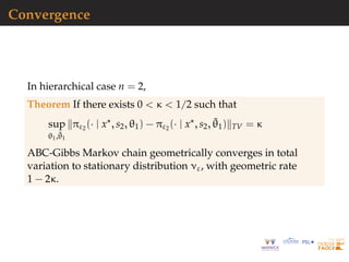
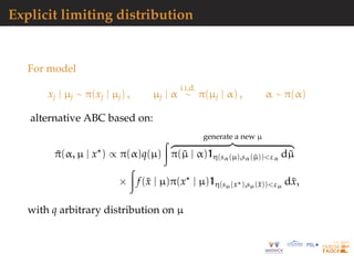
89. Explicit limiting distribution
For model
xj | µj ∼ π(xj | µj) , µj | α
i.i.d.
∼ π(µj | α) , α ∼ π(α)
Resulting Gibbs sampler stationary for posterior proportional
to
π(α, µ) q(sα(µ))
projection
f(sµ(x ) | µ)
projection
that is, for likelihood associated with sµ(x ) and prior
distribution proportional to π(α, µ)q(sα(µ)) [exact!]

90. Gibbs with ABC approximations
Souza Rodrigues et al. (arxiv:1906.04347) alternative ABC-ed
Gibbs:
Further references to earlier occurrences of Gibbs versions
of ABC
ABC version of Gibbs sampling with approximations to
the conditionals with no further corrections
Related to regression post-processing `a la Beaumont et al.
(2002) used to designing approximate full conditional,
possibly involving neural networks
Requires preliminary ABC step
Drawing from approximate full conditionals done exactly,
possibly via a bootstrapped version.

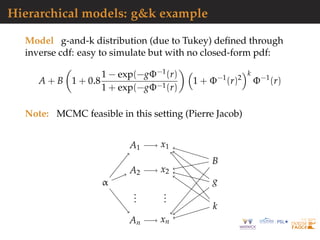
91. Hierarchical models: toy example
Model
α ∼ U([0 ; 20]),
(µ1, . . . , µn) | α ∼ N(α, 1)⊗n,
(xi,1, . . . , xi,K) | µi ∼ N (µi, 0.1)⊗K
.
Numerical experiment
n = 20, K = 10,
Pseudo observation generated for α = 1.7,
Algorithms runs for a constant budget:
Ntot = N × Nε = 21000.
We look at the estimates for µ1 whose value for the pseudo
observations is 3.04.

92. Hierarchical models: toy example
Illustration
Assumptions of convergence theorem hold
Tolerance as quantile of distances at each call, i..e, selection
of simulation with smallest distance out of Nα = Nµ = 30
Summary statistic as empirical mean (sufficient)
Setting when SMC-ABC fails as well

93. Hierarchical models: toy example
Figure comparison of the sampled densities of µ1 (left) and α
(right) [dot-dashed line as true posterior]
0
1
2
3
4
0 2 4 6
0.0
0.5
1.0
1.5
2.0
−4 −2 0 2 4
Method ABC Gibbs Simple ABC

94. Hierarchical models: toy example
Figure posterior densities of µ1 and α for 100 replicas of 3
ABC algorithms [true marginal posterior as dashed line]
ABC−GibbsSimpleABCSMC−ABC
0 2 4 6
0
1
2
3
4
0
1
2
3
4
0
10
20
30
40
mu1
density
ABC−GibbsSimpleABCSMC−ABC
0 1 2 3 4 5
0.0
0.5
1.0
1.5
2.0
2.5
0.0
0.5
1.0
1.5
2.0
0
5
10
15
20
hyperparameter
density

95. Hierarchical models: moving average example
Pseudo observations xobs
1 generated for µ1 = (−0.06, −0.22).
0
1
2
3
−1.0 −0.5 0.0 0.5 1.0
value
density
type
ABCGibbs
ABCsimple
prior
1st parameter, 1st coordinate
−1.0
−0.5
0.0
0.5
1.0
−1.0 −0.5 0.0 0.5 1.0
b1
b2
0.2
0.4
0.6
0.8
level
1st parameter simple
−1.0
−0.5
0.0
0.5
1.0
−1.0 −0.5 0.0 0.5 1.0
b1
b2
2.5
5.0
7.5
10.0
level
1st parameter gibbs
Separation from the prior for identical number of
simulations.

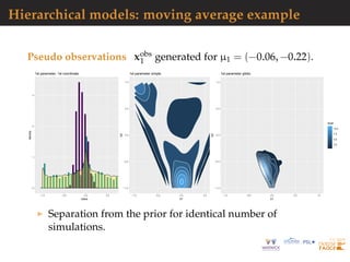
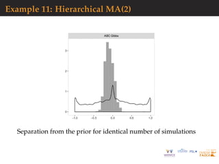
96. Hierarchical models: moving average example
Real dataset measures of 8GHz daily flux intensity emitted by
7 stellar objects from the NRL GBI website:
http://ese.nrl.navy.mil/.
[?]
0
1
2
3
−1.0 −0.5 0.0 0.5 1.0
value
density
type
ABCGibbs
ABCsimple
prior
1st parameter, 1st coordinate
−1.0
−0.5
0.0
0.5
1.0
−1.0 −0.5 0.0 0.5 1.0
b1
b2
0.2
0.4
0.6
level
1st parameter simple
−1.0
−0.5
0.0
0.5
1.0
−1.0 −0.5 0.0 0.5 1.0
b1
b2
2
4
6
8
level
1st parameter gibbs
Separation from the prior for identical number of
simulations.

97. Hierarchical models: g&k example
Model g-and-k distribution (due to Tukey) defined through
inverse cdf: easy to simulate but with no closed-form pdf:
A + B 1 + 0.8
1 − exp(−gΦ−1(r)
1 + exp(−gΦ−1(r)
1 + Φ−1
(r)2
k
Φ−1
(r)
Note: MCMC feasible in this setting (Pierre Jacob)
α
A1
A2
...
An
x1
x2
xn
...
B
g
k

98. Hierarchical models: g&k example
Assumption B, g and k known, inference on α and Ai solely.
1 2 3 4 Hyperparameter
−7.5 −7.0 −6.5 −6.0 −5.5 −5.0−7.5 −7.0 −6.5 −6.0 −5.5 −5.0−7.5 −7.0 −6.5 −6.0 −5.5 −5.0−7.5 −7.0 −6.5 −6.0 −5.5 −5.0−7.5 −7.0 −6.5 −6.0 −5.5 −5.0
0
2
4
6
8
value
density
Method ABC Gibbs ABC−SMC vanilla ABC

99. General case: inverse problem
Example inspired by deterministic inverse problems:
difficult to tackle with traditional methods
pseudo-likelihood extremely expensive to compute
requiring the use of surrogate models
Let y be solution of heat equation on a circle defined for
(τ, z) ∈]0, T] × [0, 1[ by
∂τy(z, τ) = ∂z (θ(z)∂zy(z, τ)) ,
with
θ(z) =
n
j=1
θj1[(j−1)/n,j/n](z)
and boundary conditions y(z, 0) = y0(z) and y(0, τ) = y(1, τ)
[?]

100. General case: inverse problem
Assume y0 known and parameter θ = (θ1, . . . , θn), with
discretized equation via first order finite elements of size 1/n
for z and ∆ for τ.
Stepwise approximation of solution
^y(z, t) =
n
j=1
yj,tϕj(z)
where, for j < n,
ϕj(z) = (1 − |nz − j|)1|nz−j|<1
and
ϕn(z) = (1 − nz)10<z<1/n + (nz − n + 1)11−1/n<z<1
and with yj,t defined by
yj,t+1 − yj,t
3∆
+
yj+1,t+1 − yj+1,t
6∆
+
yj−1,t+1 − yj−1,t
6∆
= yj,t+1(θj+1 + θj) − yj−1,t+1θj − yj+1,t+1θj+1.

101. General case: inverse problem
In ABC-Gibbs, each parameter θm updated with summary
statistics observations at locations m − 2, m − 1, m, m + 1 while
ABC-SMC relies on the whole data as statistic. In experiment,
n = 20 and ∆ = 0.1, with a prior θj ∼ U[0, 1], independently.
Convergence theorem applies to this setting.
Comparison with ABC, using same simulation budget, keeping
the total number of simulations constant at Nε · N = 8 · 106.
Choice of ABC reference table size critical: for a fixed
computational budget reach balance between quality of the
approximations of the conditionals (improved by increasing
Nε), and Monte-Carlo error and convergence of the algorithm,
(improved by increasing N).

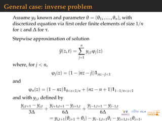
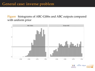
102. General case: inverse problem
Figure mean and variance of the ABC and ABC-Gibbs
estimators of θ1 as Nε increases [horizontal line shows true
value]
0.5
0.6
0.7
0.8
0 10 20 30 40
0.000
0.002
0.004
0 10 20 30 40
Method ABC Gibbs Simple ABC

103. General case: inverse problem
Figure histograms of ABC-Gibbs and ABC outputs compared
with uniform prior
ABC Gibbs Simple ABC
0.25 0.50 0.75 1.00 0.25 0.50 0.75 1.00
0
1
2
3

104. ABC postdoc positions
2 post-doc positions with the ABSint research grant:
Focus on approximate Bayesian techniques like ABC,
variational Bayes, PAC-Bayes, Bayesian non-parametrics,
scalable MCMC, and related topics. A potential direction
of research would be the derivation of new Bayesian tools
for model checking in such complex environments.
Terms: up to 24 months, no teaching duty attached,
primarily located in Universit´e Paris-Dauphine, with
supported periods in Oxford (J. Rousseau) and visits to
Montpellier (J.-M. Marin). No hard deadline.
If interested, send application to me:
bayesianstatistics@gmail.com