The document discusses the concepts of normal distribution and the 68%-95%-99.7% rule, emphasizing how sample data and z-scores can help make inferences about a population. It explains the importance of the sampling distribution of the sample mean and the central limit theorem, which states that with a sufficiently large sample size, the distribution of sample means will approximate a normal distribution. Additionally, it covers the calculation of probabilities related to sample means and their significance in statistics.

1. Statistics

2. What’s normal?
68%- 95%-99.7% Rule

3. What’s normal?
68%- 95%-99.7% Rule
• When we looked at “What’s Normal?” a couple of weeks ago, we looked at a normal distribution
and then at our sample to make some decisions about where we might fit in.
• We made decisions about what was likely – or unlikely – using our 68% -95%-99.7% Rule.
• Values WITHIN 2 sds of the mean are considered likely, or usual. Anything MORE than 2sds away
from the mean – either lower or higher – are considered unlikely, or unusual.
• And we can make a couple of conclusions from this.
• The first is that our sample DOES NOT BELONG TO THIS POPULATION – maybe we got a young child
mixed up with our adult population. But since we were careful in only using ADULTS, we’re pretty
sure that we haven’t made an error.
• The second is that something in the population has changed. If our IQ score was 135 it’s in the
unlikely range. But just maybe, we’re getting smarter and the average adult IQ is no longer 100.
• The normal distribution is what is normal in the population.
• But most of the time, we use samples to make decisions, so we need to look at sample distributions
– and the theory behind it ...

4. Sampling Distribution
• Using z-scores, we are able to describe where a ‘score’ is located in a
distribution
• z-scores and probabilities covered so far comprise information
about a single score
• z-scores are also useful for determining where sample statistics falls
within a distribution
• Sample mean / Sample proportion

5. Sampling Distribution
• Is sample truly represent population…?
• Multiple samples may differ slightly..
• Differences between samples is called sampling variability.
• If we take lots of random samples from the population, we can build a
picture of the samples – a sampling distribution.

6. Distribution of sample means
• The distribution of sample means is ALL possible random samples of n = #?
obtained from a population
• Entire population would be covered with samples
• Need all possible random sample values to be able to calculate probability
• Each sample we take will differ from another so need to be aware of sampling error –
‘natural’ discrepancy between sample statistics and population parameters
• We need a method to make a decision about which sample might truly represent the
population …

7. Distribution of sample means
• The distribution of sample means, often referred to as the sampling
distribution of the sample mean, describes how the means of
multiple samples (of the same size) drawn from a population are
distributed. This concept is crucial for making inferences about a
population based on sample data.
• If you take many samples from a population and calculate the mean
of each sample, the distribution of those sample means will tend to
be normal (or nearly normal), especially as the sample size n becomes
larger

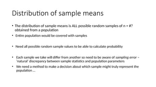
8. Distribution of sample means-Characteristics
• Sample means should cluster around the population mean
• Should form a normal distribution
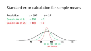
• The larger the sample size, the narrower the distribution
• That is, the closer the sample mean should be to the
population mean
• More information, so can be more concise
• When we have larger populations / samples, calculations can
become cumbersome, as we are using all possible samples [and if
we can actually obtain all possible samples]

9. Central Limit Theorem
• The Central Limit Theorem states that, regardless of the population
distribution, the sampling distribution of the sample mean will approximate
a normal distribution if the sample size is sufficiently large. This is true as
long as the samples are independent and drawn from the same population
• If the samples are taken from a normally distributed population, they should also be
normally distributed
• Regardless of the shape of the original distribution, if the sample size is n ≥ 30, the sampling
distribution is almost ‘perfectly normal’
Central Tendency:
• The mean of the Distribution of Sample Means equals the mean of the population
= μ
Variability:
• The standard deviation of the samples [standard error] depends on the size of the samples

10. Distribution of sample means
Shape: » Normal distribution
Central Tendency: » = μ

11. Standard error calculation for sample means
IQ scores for a population of university students are normally
distributed μ = 110 and standard deviation = 15
Sample size of 9: Sample size of 100:

12. Standard error calculation for sample means
Population: μ = 100 σ = 15
Sample size of 9: = 100 = 5
Sample size of 25: = 100 = 3
70 85 100 115 130
90 95 100 105 110
94 97 100 103 106

13. Probability and the Distribution of sample means
• Standardizing the distribution of sample means allows us to calculate
the probability associated with any specific sample
z =
• = [standard deviation of the sampling distribution
• μ = population mean = Sample mean
• The primary use of the distribution of sample means is to calculate
the probability associated with any specific sample

14. Probability and the Distribution of sample mean
Example: Heights of a population of women are normally distributed:
μ = 160 and standard deviation = 8cm
• You take a random sample of n = 16 women from this population. What
is the probability that their mean height will be less than 158 cm?
• Distribution of sample means is normally distributed
• Distribution of sample mean is equal to population mean M = 160
• Standard error needs to be calculated … then the z score …
‐
Standard error: = = 2
z score calculation:
‐ z = = -1

15. Probability and the Distribution of sample mean
What is the probability that their mean height will be less than 158 cm?
• Distribution of sample mean is equal to population mean M = 160
• Standard error =2
• z score = 1
‐ ‐
Probability = 13.59% + 2.28% = 15.87%
OR
Table B.1 P(z<-1)=0.1587
OR
“15.87% of random samples of size 16 from this population will have a mean height that is
less than 158cm”

16. Probability and the Distribution of sample mean
What range of values would be expected 95% of the time if the sample
size were n=16?
With n=16 the standard error is = =2 cm. Using z=±1.96, the 95% range
extends from 156.08 to 162.92 cm.
160+(1.96 )= 160+(1.96×2)=163.92 cm
160 - (1.96 )= 160 - (1.96×2)=156.08 cm

17. Probability and the Distribution of sample mean

18. Sampling Distribution for Proportions
• Sampling distributions for proportions are fundamental in statistics,
especially when dealing with categorical data.
• Sampling distribution proportion equals population proportion
• The standard deviation of the samples [standard error] depends on
sample size …

19. Sampling Distribution for Proportions
• Population proportion (𝑝): This is the proportion of the population
that has a certain characteristic. For example, if you’re studying the
proportion of voters who support a specific candidate, would be
𝑝
the true proportion of all voters who support that candidate.
• Sample proportion ( )
𝑝 ̂ This is the proportion of individuals in a
sample who have the characteristic of interest. For instance, if you
survey 100 voters and 60 support the candidate, ​ would be 0.6 or
60%.