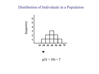
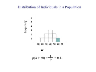
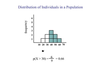
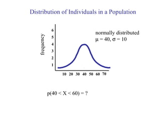
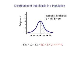
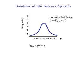
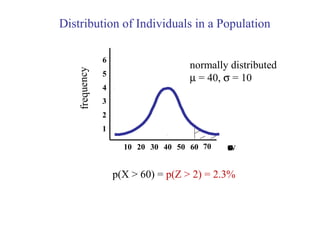
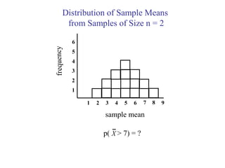
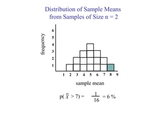
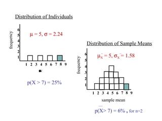
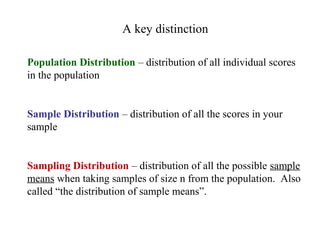
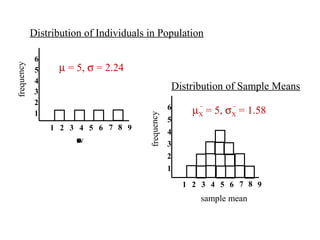
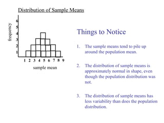
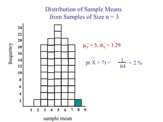
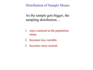
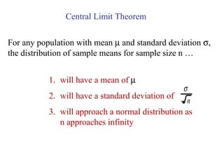
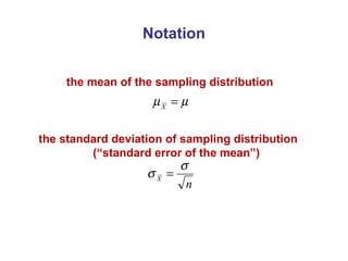
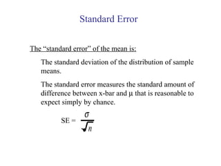
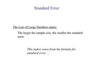
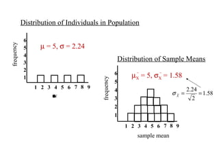
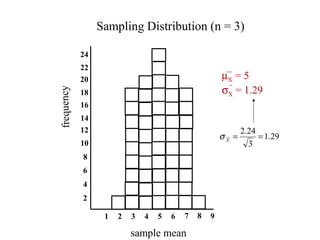
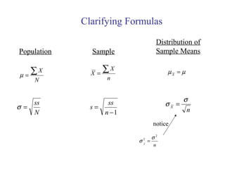
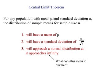
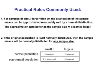
- The document discusses key concepts related to probability and sampling, including sampling distributions, the central limit theorem, and standard error. - As sample size increases, the sampling distribution becomes more normal in shape and less variable, with a standard deviation that approaches the population standard deviation divided by the square root of the sample size. - The central limit theorem states that for large sample sizes, the distribution of sample means will approximate a normal distribution, even if the population is not normally distributed. This allows probabilities to be calculated for sample means.

1. Probability and Samples
• Sampling Distributions
• Central Limit Theorem
• Standard Error
• Probability of Sample Means

2. Sample Population
Inferential Statistics
Probability
last week and today
tomorrow and beyond

3. - getting a certain type of individual when we
sample once
- getting a certain type of sample mean when n>1
When we take a sample from a population we can talk
about the probability of
today
last Thursday

4. p(X > 50) = ?
10 20 30 40 50 60
1
2
3
frequency 4
5
6
rawscore
70
Distribution of Individuals in a Population

5. 10 20 30 40 50 60
1
2
3
frequency 4
5
6
rawscore
70
p(X > 50) =
1
9
= 0.11
Distribution of Individuals in a Population

6. p(X > 30) = ?
10 20 30 40 50 60
1
2
3
frequency 4
5
6
rawscore
70
Distribution of Individuals in a Population

7. p(X > 30) =
6
9
= 0.66
10 20 30 40 50 60
1
2
3
frequency 4
5
6
rawscore
70
Distribution of Individuals in a Population

8. 10 20 30 40 50 60
1
2
3
frequency 4
5
6
70
normally distributed
µ = 40, σ = 10
Distribution of Individuals in a Population
p(40 < X < 60) = ?

9. 10 20 30 40 50 60
1
2
3
frequency 4
5
6
70
normally distributed
µ = 40, σ = 10
p(40 < X < 60) = p(0 < Z < 2) = 47.7%
Distribution of Individuals in a Population

10. 10 20 30 40 50 60
1
2
3
frequency 4
5
6
70
normally distributed
µ = 40, σ = 10
rawscore
Distribution of Individuals in a Population
p(X > 60) = ?

11. 10 20 30 40 50 60
1
2
3
frequency 4
5
6
rawscore70
normally distributed
µ = 40, σ = 10
p(X > 60) = p(Z > 2) = 2.3%
Distribution of Individuals in a Population

12. For the preceding calculations to be accurate, it is
necessary that the sampling process be random.
A random sample must satisfy two requirements:
1. Each individual in the population has an equal
chance of being selected.
2. If more than one individual is to be selected, there
must be constant probability for each and every
selection (i.e. sampling with replacement).

13. A distribution of sample means is:
the collection of sample means for all the possible
random samples of a particular size (n) that can be
obtained from a population.
Distribution of Sample Means

14. Population
1 2 3 4 5 6
1
2
3
frequency 4
5
6
rawscore
7 8 9

15. Distribution of Sample Means
from Samples of Size n = 2
1 2, 2 2
2 2,4 3
3 2,6 4
4 2,8 5
5 4,2 3
6 4,4 4
7 4,6 5
8 4,8 6
9 6,2 4
10 6,4 5
11 6,6 6
12 6,8 7
13 8,2 5
14 8,4 6
15 8.6 7
16 8.8 8
Sample # Scores Mean ( )X

16. Distribution of Sample Means
from Samples of Size n = 2
1 2 3 4 5 6
1
2
3
frequency 4
5
6
7 8 9
sample mean
We can use the distribution of sample means to answer
probability questions about sample means

17. Distribution of Sample Means
from Samples of Size n = 2
1 2 3 4 5 6
1
2
3
frequency 4
5
6
7 8 9
sample mean
p( > 7) = ?X

18. Distribution of Sample Means
from Samples of Size n = 2
1 2 3 4 5 6
1
2
3
frequency 4
5
6
7 8 9
sample mean
p( > 7) = 1
16
= 6 %X

19. 1 2 3 4 5 6
1
2
3
frequency
4
5
6
rawscore
7 8 9
Distribution of Individuals in Population
Distribution of Sample Means
1 2 3 4 5 6
1
2
3
frequency
4
5
6
7 8 9
sample mean
µ = 5, σ = 2.24
µX = 5, σX = 1.58

20. 1 2 3 4 5 6
1
2
3
frequency
4
5
6
rawscore
7 8 9
1 2 3 4 5 6
1
2
3
frequency
4
5
6
7 8 9
sample mean
Distribution of Individuals
Distribution of Sample Means
µ = 5, σ = 2.24
p(X > 7) = 25%
µX = 5, σX = 1.58
p(X> 7) = 6% , for n=2

21. A key distinction
Population Distribution – distribution of all individual scores
in the population
Sample Distribution – distribution of all the scores in your
sample
Sampling Distribution – distribution of all the possible sample
means when taking samples of size n from the population. Also
called “the distribution of sample means”.

22. 1 2 3 4 5 6
1
2
3
frequency
4
5
6
rawscore
7 8 9
Distribution of Individuals in Population
Distribution of Sample Means
1 2 3 4 5 6
1
2
3
frequency
4
5
6
7 8 9
sample mean
µ = 5, σ = 2.24
µX = 5, σX = 1.58

23. 1 2 3 4 5 6
1
2
3
frequency
4
5
6
7 8 9
sample mean
Distribution of Sample Means
Things to Notice
1. The sample means tend to pile up
around the population mean.
2. The distribution of sample means is
approximately normal in shape, even
though the population distribution was
not.
3. The distribution of sample means has
less variability than does the population
distribution.

24. What if we took a larger sample?

25. Distribution of Sample Means
from Samples of Size n = 3
1 2 3 4 5 6
2
4
6
frequency
8
10
12
7 8 9
sample mean
14
16
18
20
22
24
1
64
= 2 %
µX = 5, σX = 1.29
p( X > 7) =

26. Distribution of Sample Means
As the sample gets bigger, the
sampling distribution…
1. stays centered at the population
mean.
2. becomes less variable.
3. becomes more normal.

27. Central Limit Theorem
For any population with mean µ and standard deviation σ,
the distribution of sample means for sample size n …
1. will have a mean of µ
2. will have a standard deviation of
3. will approach a normal distribution as
n approaches infinity
σ
n

28. Notation
the mean of the sampling distribution
the standard deviation of sampling distribution
(“standard error of the mean”)
µµ =X
n
X
σ
σ =

29. The “standard error” of the mean is:
The standard deviation of the distribution of sample
means.
The standard error measures the standard amount of
difference between x-bar and µ that is reasonable to
expect simply by chance.
Standard Error
SE =
σ
n

30. The Law of Large Numbers states:
The larger the sample size, the smaller the standard
error.
Standard Error
This makes sense from the formula for
standard error …

31. 1 2 3 4 5 6
1
2
3
frequency
4
5
6
rawscore
7 8 9
Distribution of Individuals in Population
Distribution of Sample Means
1 2 3 4 5 6
1
2
3
frequency
4
5
6
7 8 9
sample mean
µ = 5, σ = 2.24
µX = 5, σX = 1.58
58.1
2
24.2
==X
σ

32. 1 2 3 4 5 6
2
4
6
frequency
8
10
12
7 8 9
sample mean
14
16
18
20
22
24
Sampling Distribution (n = 3)
µX = 5
σX = 1.29
29.1
3
24.2
==X
σ

33. Population Sample
Distribution of
Sample Means
Clarifying Formulas
N
X∑=µ n
X
X
∑= µµ =X
N
ss
=σ
1−
=
n
ss
s n
X
σ
σ =
nX
2
2 σ
σ =
notice

34. Central Limit Theorem
For any population with mean µ and standard deviation σ,
the distribution of sample means for sample size n …
1. will have a mean of µ
2. will have a standard deviation of
3. will approach a normal distribution as
n approaches infinity
σ
n
What does this mean in
practice?

35. Practical Rules Commonly Used:
1. For samples of size n larger than 30, the distribution of the sample
means can be approximated reasonably well by a normal distribution.
The approximation gets better as the sample size n becomes larger.
2. If the original population is itself normally distributed, then the sample
means will be normally distributed for any sample size.
small n large n
normal population
non-normal population
normalisX normalisX
normalisXnonnormalisX

36. Probability and the Distribution of Sample
Means
The primary use of the distribution of sample
means is to find the probability associated with any
specific sample.

37. Probability and the Distribution of Sample
Means
Given the population of women has normally
distributed weights with a mean of 143 lbs and
a standard deviation of 29 lbs,
Example:
1. if one woman is randomly selected, find the probability that her
weight is greater than 150 lbs.
2. if 36 different women are randomly selected, find the probability
that their mean weight is greater than 150 lbs.

38. 0 0.24
Given the population of women has normally distributed
weights with a mean of 143 lbs and a standard deviation of
29 lbs,
1. if one woman is randomly selected, find the probability that her
weight is greater than 150 lbs.
0.4052
150µ = 143
σ = 29
Population distribution
z = 150-143 = 0.24
29

39. 0 1.45
Given the population of women has normally distributed
weights with a mean of 143 lbs and a standard deviation of
29 lbs,
0.0735
2. if 36 different women are randomly selected, find the probability
that their mean weight is greater than 150 lbs.
36
29
=X
σ
150µ = 143
σ = 4.33
Sampling distribution
z = 150-143 = 1.45
4.33

40. Probability and the Distribution of Sample
Means
Given the population of women has normally
distributed weights with a mean of 143 lbs and
a standard deviation of 29 lbs,
Example:
1. if one woman is randomly selected, find the probability that her
weight is greater than 150 lbs.
2. if 36 different women are randomly selected, find the probability
that their mean weight is greater than 150 lbs.
41.)150( =>XP
07.)150( =>XP

41. Practice
Given a population of 400 automobile models,
with a mean horsepower = 105 HP, and a
standard deviation = 40 HP,
Example:
1. What is the standard error of the sample mean for a sample of
size 1?
2. What is the standard error of the sample mean for a sample of
size 4?
3. What is the standard error of the sample mean for a sample of
size 25?
40
20
8

42. Example:
1. if one model is randomly selected from the population, find the
probability that its horsepower is greater than 120.
2. If 4 models are randomly selected from the population, find the
probability that their mean horsepower is greater than 120
3. If 25 models are randomly selected from the population, find the
probability that their mean horsepower is greater than 120
Practice
Given a population of 400 automobile models,
with a mean horsepower = 105 HP, and a
standard deviation = 40 HP,
.35
.23
.03