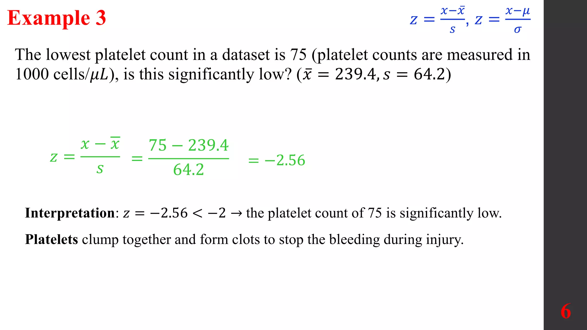
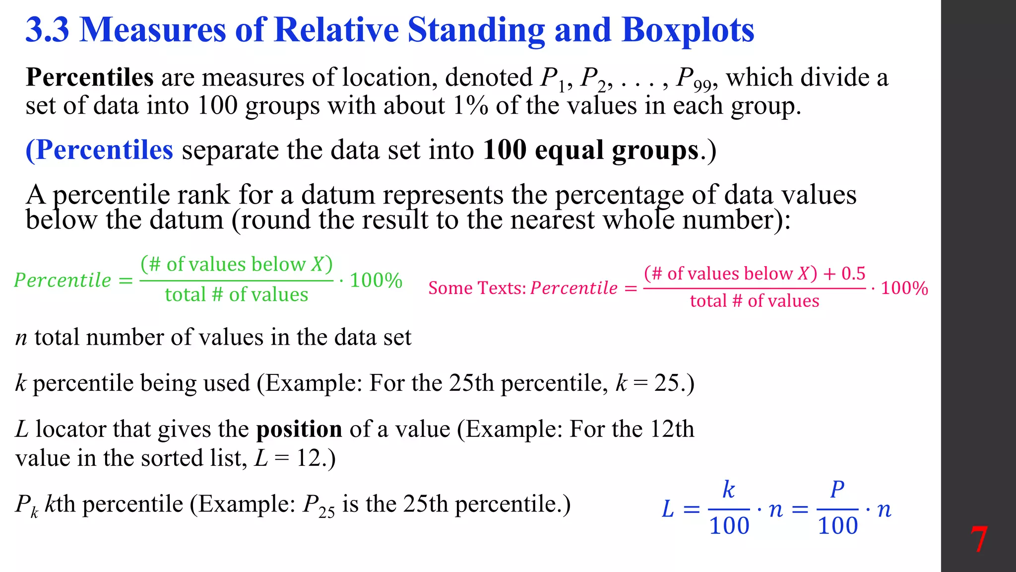
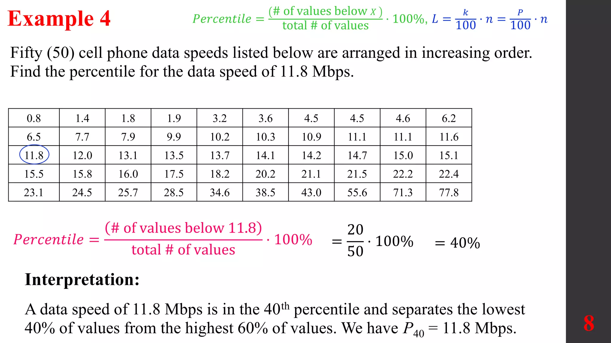
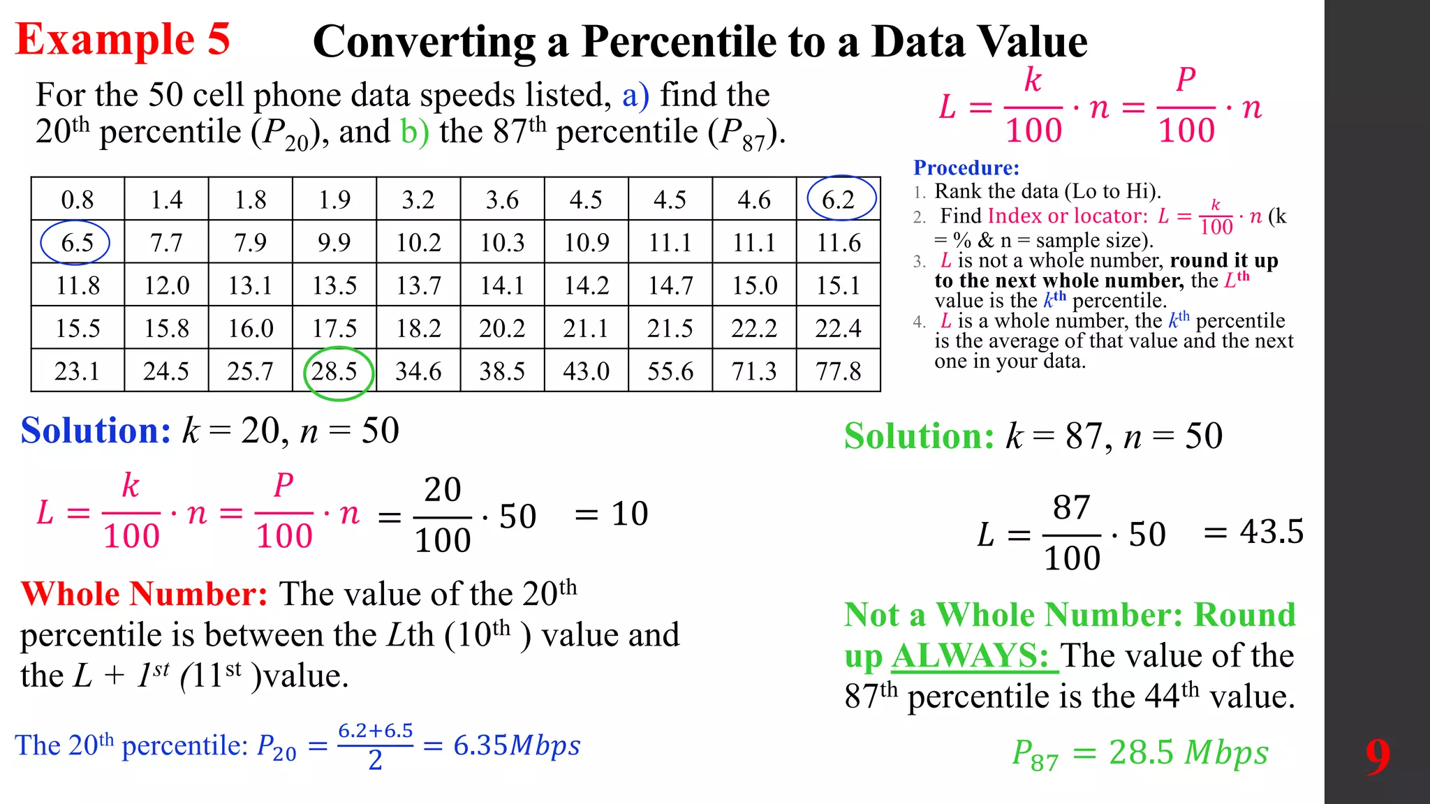
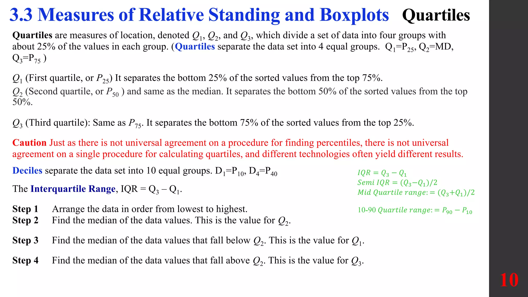
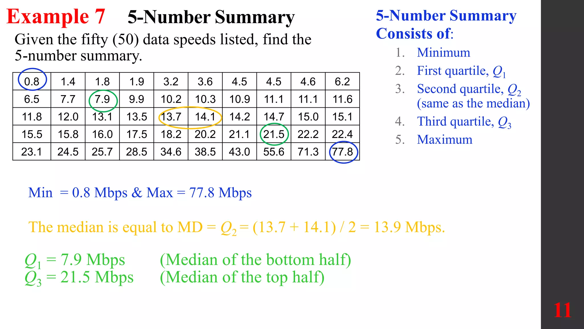
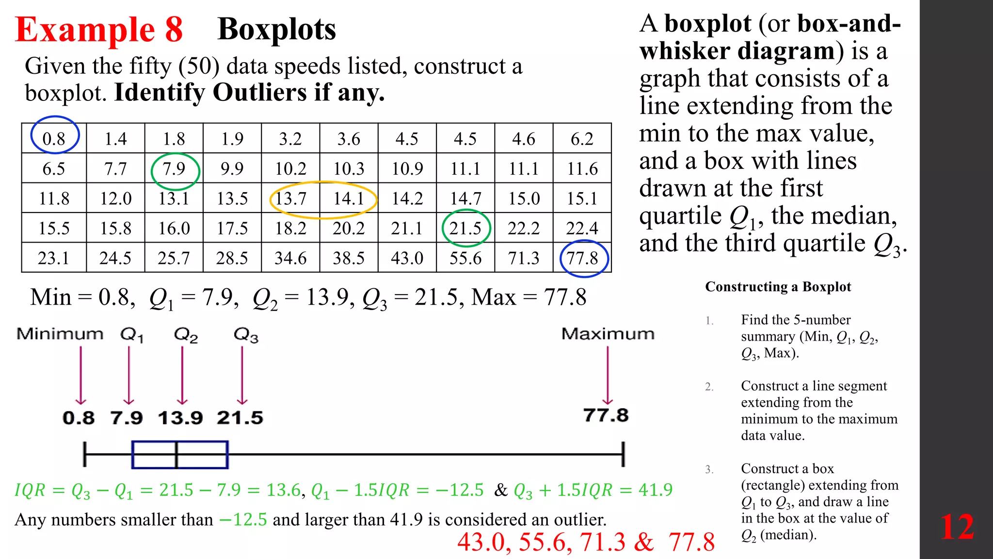
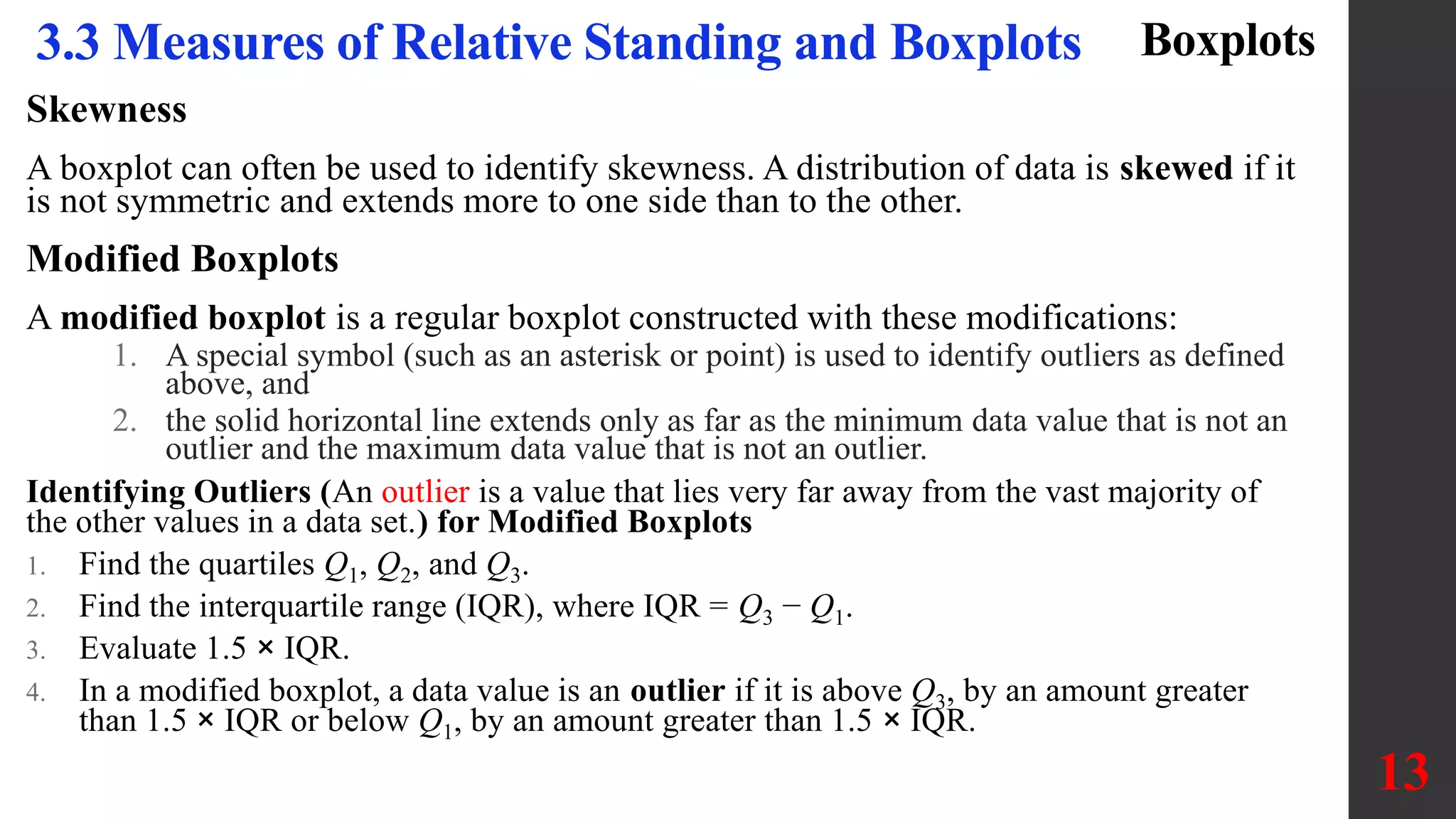
Chapter 3 discusses various statistical measures for describing, exploring, and comparing data, focusing on central tendency, variation, and relative standing using techniques like z-scores, percentiles, and quartiles. It emphasizes the use of boxplots and five-number summaries to visualize data distribution, identify outliers, and understand data skewness. Key concepts include calculating measures like the mean, median, mode, and employing formulas for z-scores and percentiles to assess individual data values' positions within a dataset.

1. Elementary Statistics
Chapter 3:
Describing, Exploring,
and Comparing Data
3.3 Measures of
Relative Standing and
Boxplots
1

2. Chapter 3:
Describing, Exploring, and Comparing Data
3.1 Measures of Center
3.2 Measures of Variation
3.3 Measures of Relative Standing and Boxplots
2
Objectives:
1. Summarize data, using measures of central tendency, such as the mean, median, mode,
and midrange.
2. Describe data, using measures of variation, such as the range, variance, and standard
deviation.
3. Identify the position of a data value in a data set, using various measures of position,
such as percentiles, deciles, and quartiles.
4. Use the techniques of exploratory data analysis, including boxplots and five-number
summaries, to discover various aspects of data

3. z Scores
A z score (or standard score or standardized value) is the number of standard
deviations that a given value x is above or below the mean. It is obtained by subtracting
the mean from the value and dividing the result by the standard deviation.
Sample: 𝑧 =
𝑥−𝑥
𝑠
Population:𝑧 =
𝑥−𝜇
𝜎
3.3 Measures of Relative Standing and Boxplots
Values: z scores ≤ −2.00 or z scores ≥ 2.00 3
Important Properties of z Scores
1. A z score is the number of standard deviations that a given value x is above or below the mean.
2. z scores are expressed as numbers with no units of measurement.
3. A data value is significantly low if its z score is less than or equal to −2 or the value is
significantly high if its z score is greater than or equal to +2.
4. If an individual data value is less than the mean, its corresponding z score is a negative number.

4. Example 1
4
Which of the following two data values is more extreme relative to the data
set from which it came?
=
4000 − 3152
693.4
= 1.22
=
99 − 98.20
0.62
= 1.29
Temperature
The 4000 g weight of a baby (n = 400, 𝑥 = 3152.0𝑔, 𝑠 = 693.4𝑔)
The 990
𝐹 temperature of an adult (n = 106, 𝑥 = 98.200
𝐹, 𝑠 = 0.620
𝐹)
𝑧 =
𝑥 − 𝑥
𝑠
𝑧 =
𝑥−𝑥
𝑠
, 𝑧 =
𝑥−𝜇
𝜎

5. 5
A student scored 65 on a calculus test that had a mean of 50 and a standard
deviation of 10; she scored 30 on a history test with a mean of 25 and a
standard deviation of 5. Compare her relative positions on the two tests.
She has a higher relative position in the Calculus class.
History: 𝑧 =
30 − 25
5
Calculus: 𝑧 =
65 − 50
10
= 1.5
= 1.0
𝑧 =
𝑥 − 𝜇
𝜎
Example 2 𝑧 =
𝑥−𝑥
𝑠
, 𝑧 =
𝑥−𝜇
𝜎

6. 6
=
75 − 239.4
64.2
= −2.56
Interpretation: 𝑧 = −2.56 < −2 → the platelet count of 75 is significantly low.
Platelets clump together and form clots to stop the bleeding during injury.
The lowest platelet count in a dataset is 75 (platelet counts are measured in
1000 cells/𝜇𝐿), is this significantly low? (𝑥 = 239.4, 𝑠 = 64.2)
𝑧 =
𝑥 − 𝑥
𝑠
Example 3 𝑧 =
𝑥−𝑥
𝑠
, 𝑧 =
𝑥−𝜇
𝜎

7. Percentiles are measures of location, denoted P1, P2, . . . , P99, which divide a
set of data into 100 groups with about 1% of the values in each group.
(Percentiles separate the data set into 100 equal groups.)
A percentile rank for a datum represents the percentage of data values
below the datum (round the result to the nearest whole number):
3.3 Measures of Relative Standing and Boxplots
𝑃𝑒𝑟𝑐𝑒𝑛𝑡𝑖𝑙𝑒 =
# of values below 𝑋
total # of values
⋅ 100% Some Texts: 𝑃𝑒𝑟𝑐𝑒𝑛𝑡𝑖𝑙𝑒 =
# of values below 𝑋 + 0.5
total # of values
⋅ 100%
n total number of values in the data set
k percentile being used (Example: For the 25th percentile, k = 25.)
L locator that gives the position of a value (Example: For the 12th
value in the sorted list, L = 12.)
Pk kth percentile (Example: P25 is the 25th percentile.)
7
𝐿 =
𝑘
100
⋅ 𝑛 =
𝑃
100
⋅ 𝑛

8. 8
Fifty (50) cell phone data speeds listed below are arranged in increasing order.
Find the percentile for the data speed of 11.8 Mbps.
0.8 1.4 1.8 1.9 3.2 3.6 4.5 4.5 4.6 6.2
6.5 7.7 7.9 9.9 10.2 10.3 10.9 11.1 11.1 11.6
11.8 12.0 13.1 13.5 13.7 14.1 14.2 14.7 15.0 15.1
15.5 15.8 16.0 17.5 18.2 20.2 21.1 21.5 22.2 22.4
23.1 24.5 25.7 28.5 34.6 38.5 43.0 55.6 71.3 77.8
𝑃𝑒𝑟𝑐𝑒𝑛𝑡𝑖𝑙𝑒 =
# of values below 11.8
total # of values
⋅ 100% =
20
50
⋅ 100% = 40%
Interpretation:
A data speed of 11.8 Mbps is in the 40th percentile and separates the lowest
40% of values from the highest 60% of values. We have P40 = 11.8 Mbps.
Example 4 𝑃𝑒𝑟𝑐𝑒𝑛𝑡𝑖𝑙𝑒 =
# of values below 𝑋
total # of values
⋅ 100%, 𝐿 =
𝑘
100
⋅ 𝑛 =
𝑃
100
⋅ 𝑛

9. Example 5
9
For the 50 cell phone data speeds listed, a) find the
20th percentile (P20), and b) the 87th percentile (P87).
0.8 1.4 1.8 1.9 3.2 3.6 4.5 4.5 4.6 6.2
6.5 7.7 7.9 9.9 10.2 10.3 10.9 11.1 11.1 11.6
11.8 12.0 13.1 13.5 13.7 14.1 14.2 14.7 15.0 15.1
15.5 15.8 16.0 17.5 18.2 20.2 21.1 21.5 22.2 22.4
23.1 24.5 25.7 28.5 34.6 38.5 43.0 55.6 71.3 77.8
Converting a Percentile to a Data Value
𝐿 =
𝑘
100
⋅ 𝑛 =
𝑃
100
⋅ 𝑛
Solution: k = 20, n = 50
=
20
100
⋅ 50
Whole Number: The value of the 20th
percentile is between the Lth (10th ) value and
the L + 1st (11st )value.
The 20th percentile: 𝑃20 =
6.2+6.5
2
= 6.35𝑀𝑏𝑝𝑠
Procedure:
1. Rank the data (Lo to Hi).
2. Find Index or locator: 𝐿 =
𝑘
100
⋅ 𝑛 (k
= % & n = sample size).
3. 𝐿 is not a whole number, round it up
to the next whole number, the Lth
value is the kth percentile.
4. 𝐿 is a whole number, the kth percentile
is the average of that value and the next
one in your data.
𝐿 =
𝑘
100
⋅ 𝑛 =
𝑃
100
⋅ 𝑛 = 10
Solution: k = 87, n = 50
𝐿 =
87
100
⋅ 50 = 43.5
Not a Whole Number: Round
up ALWAYS: The value of the
87th percentile is the 44th value.
𝑃87 = 28.5 𝑀𝑏𝑝𝑠

10. Quartiles
Quartiles are measures of location, denoted Q1, Q2, and Q3, which divide a set of data into four groups with
about 25% of the values in each group. (Quartiles separate the data set into 4 equal groups. Q1=P25, Q2=MD,
Q3=P75 )
Q1 (First quartile, or P25) It separates the bottom 25% of the sorted values from the top 75%.
Q2 (Second quartile, or P50 ) and same as the median. It separates the bottom 50% of the sorted values from the top
50%.
Q3 (Third quartile): Same as P75. It separates the bottom 75% of the sorted values from the top 25%.
Caution Just as there is not universal agreement on a procedure for finding percentiles, there is not universal
agreement on a single procedure for calculating quartiles, and different technologies often yield different results.
Deciles separate the data set into 10 equal groups. D1=P10, D4=P40
The Interquartile Range, IQR = Q3 – Q1.
Step 1 Arrange the data in order from lowest to highest.
Step 2 Find the median of the data values. This is the value for Q2.
Step 3 Find the median of the data values that fall below Q2. This is the value for Q1.
Step 4 Find the median of the data values that fall above Q2. This is the value for Q3.
10
3.3 Measures of Relative Standing and Boxplots
𝐼𝑄𝑅 = 𝑄3 − 𝑄1
𝑆𝑒𝑚𝑖 𝐼𝑄𝑅 = (𝑄3−𝑄1)/2
𝑀𝑖𝑑 𝑄𝑢𝑎𝑟𝑡𝑖𝑙𝑒 𝑟𝑎𝑛𝑔𝑒: = (𝑄3+𝑄1)/2
10-90 𝑄𝑢𝑎𝑟𝑡𝑖𝑙𝑒 𝑟𝑎𝑛𝑔𝑒: = 𝑃90 − 𝑃10

11. Example 7
11
Given the fifty (50) data speeds listed, find the
5-number summary.
0.8 1.4 1.8 1.9 3.2 3.6 4.5 4.5 4.6 6.2
6.5 7.7 7.9 9.9 10.2 10.3 10.9 11.1 11.1 11.6
11.8 12.0 13.1 13.5 13.7 14.1 14.2 14.7 15.0 15.1
15.5 15.8 16.0 17.5 18.2 20.2 21.1 21.5 22.2 22.4
23.1 24.5 25.7 28.5 34.6 38.5 43.0 55.6 71.3 77.8
5-Number Summary
Min = 0.8 Mbps & Max = 77.8 Mbps
The median is equal to MD = Q2 = (13.7 + 14.1) / 2 = 13.9 Mbps.
5-Number Summary
Consists of:
1. Minimum
2. First quartile, Q1
3. Second quartile, Q2
(same as the median)
4. Third quartile, Q3
5. Maximum
Q1 = 7.9 Mbps (Median of the bottom half)
Q3 = 21.5 Mbps (Median of the top half)

12. Example 8
12
Given the fifty (50) data speeds listed, construct a
boxplot. Identify Outliers if any.
0.8 1.4 1.8 1.9 3.2 3.6 4.5 4.5 4.6 6.2
6.5 7.7 7.9 9.9 10.2 10.3 10.9 11.1 11.1 11.6
11.8 12.0 13.1 13.5 13.7 14.1 14.2 14.7 15.0 15.1
15.5 15.8 16.0 17.5 18.2 20.2 21.1 21.5 22.2 22.4
23.1 24.5 25.7 28.5 34.6 38.5 43.0 55.6 71.3 77.8
Boxplots A boxplot (or box-and-
whisker diagram) is a
graph that consists of a
line extending from the
min to the max value,
and a box with lines
drawn at the first
quartile Q1, the median,
and the third quartile Q3.
Min = 0.8, Q1 = 7.9, Q2 = 13.9, Q3 = 21.5, Max = 77.8
Constructing a Boxplot
1. Find the 5-number
summary (Min, Q1, Q2,
Q3, Max).
2. Construct a line segment
extending from the
minimum to the maximum
data value.
3. Construct a box
(rectangle) extending from
Q1 to Q3, and draw a line
in the box at the value of
Q2 (median).
𝐼𝑄𝑅 = 𝑄3 − 𝑄1 = 21.5 − 7.9 = 13.6, 𝑄1 − 1.5𝐼𝑄𝑅 = −12.5 & 𝑄3 + 1.5𝐼𝑄𝑅 = 41.9
Any numbers smaller than −12.5 and larger than 41.9 is considered an outlier.
43.0, 55.6, 71.3 & 77.8

13. Skewness
A boxplot can often be used to identify skewness. A distribution of data is skewed if it
is not symmetric and extends more to one side than to the other.
Modified Boxplots
A modified boxplot is a regular boxplot constructed with these modifications:
1. A special symbol (such as an asterisk or point) is used to identify outliers as defined
above, and
2. the solid horizontal line extends only as far as the minimum data value that is not an
outlier and the maximum data value that is not an outlier.
Identifying Outliers (An outlier is a value that lies very far away from the vast majority of
the other values in a data set.) for Modified Boxplots
1. Find the quartiles Q1, Q2, and Q3.
2. Find the interquartile range (IQR), where IQR = Q3 − Q1.
3. Evaluate 1.5 × IQR.
4. In a modified boxplot, a data value is an outlier if it is above Q3, by an amount greater
than 1.5 × IQR or below Q1, by an amount greater than 1.5 × IQR.
13
3.3 Measures of Relative Standing and Boxplots Boxplots

14. Example 9
14
Given the fifty (50) data speeds listed, find the
40th percentile, denoted by P40.
0.8 1.4 1.8 1.9 3.2 3.6 4.5 4.5 4.6 6.2
6.5 7.7 7.9 9.9 10.2 10.3 10.9 11.1 11.1 11.6
11.8 12.0 13.1 13.5 13.7 14.1 14.2 14.7 15.0 15.1
15.5 15.8 16.0 17.5 18.2 20.2 21.1 21.5 22.2 22.4
23.1 24.5 25.7 28.5 34.6 38.5 43.0 55.6 71.3 77.8
Converting a Percentile to a Data Value (Time)
Whole Number: The value of the 40th percentile is
between the Lth (20th ) value and the 21st value.
The 40th percentile is P40 = 11.7 Mbps.
𝐿 =
𝑘
100
⋅ 𝑛 =
𝑃
100
⋅ 𝑛
Procedure:
1. Rank the data (Lo to Hi).
2. Find Index or locator: 𝐿 =
𝑘
100
⋅ 𝑛 (k
= % & n = sample size).
3. 𝐿 is not a whole number, round it up
to the next whole number, the Lth
value is the kth percentile.
4. 𝐿 is a whole number, the kth percentile
is the average of that value and the next
one in your data.
Solution: k = 40, n = 50
=
40
100
⋅ 50
𝐿 =
𝑘
100
⋅ 𝑛 =
𝑃
100
⋅ 𝑛 = 20

15. Example 10
15
A teacher gives a 20-point test to 10 students. a) Find the percentile rank of a score of
12. b) Find the value corresponding to the 25th percentile.
18, 15, 12, 6, 8, 2, 3, 5, 20, 10
100
n k
L


Sort in ascending order.
2, 3, 5, 6, 8, 10, 12, 15, 18, 20
Interpretation:
A student whose score
was 12 did better than
65% of the class.
6 values
=
6 + 0.5
10
⋅ 100% = 65%
Some Texts: 𝑃𝑒𝑟𝑐𝑒𝑛𝑡𝑖𝑙𝑒 =
# of values below 𝑋 + 0.5
total # of values
⋅ 100%
𝑃𝑒𝑟𝑐𝑒𝑛𝑡𝑖𝑙𝑒 =
# of values below 𝑋 + 0.5
total # of values
⋅ 100%
b) Sort in ascending order.
2, 3, 5, 6, 8, 10, 12, 15, 18, 20
𝑐 =
𝑛 ⋅ 𝑝
100
=
10 ⋅ 25
100
= 2.5 ≈ 3
Interpretation:
The value 5 corresponds
to the 25th percentile.