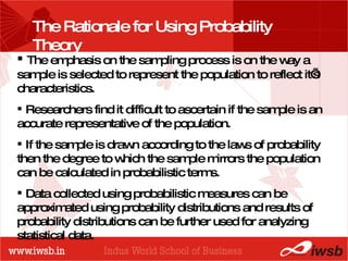
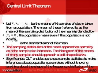
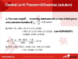
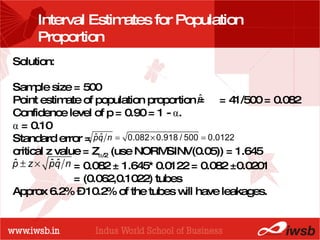
This document provides an overview of quantitative methods for probability distributions. It discusses key concepts like binomial distribution, normal distribution, standard normal distribution, central limit theorem, point estimates, interval estimates, and confidence intervals. Examples are provided to illustrate how to calculate probabilities, means, and confidence intervals for estimating population parameters based on sample data. Key probability distributions and statistical techniques are defined to analyze and make inferences about data.

1. QUANTITATIVE METHODS

2. PROBABILITY DISTRIBUTIONS The emphasis on the sampling process is on the way a sample is selected to represent the population to reflect it’s characteristics. Researchers find it difficult to ascertain if the sample is an accurate representative of the population. If the sample is drawn according to the laws of probability then the degree to which the sample mirrors the population can be calculated in probabilistic terms. Data collected using probabilistic measures can be approximated using probability distributions and results of probability distributions can be further used for analyzing statistical data. The Rationale for Using Probability Theory

3. PROBABILITY DISTRIBUTIONS Binomial Distribution Normal Distribution, Standard Normal Distribution Central Limit Theorem Estimation Confidence Intervals Estimating Sample Size In this session ….

4. PROBABILITY DISTRIBUTIONS DISCRETE CONTINUOUS e.g Binomial Distribution tosses of a coin. success or failure of students in an aptitude test. e.g Normal Distribution Frequency distribution of light bulbs measured on a continuous scale of hours.

5. - the B-school Binomial Distribution Characteristics of Bernoulli Process Each trial has two possible outcomes: success or failure. The probability of outcome is fixed over time. Trials are statistically independent: outcome of one trial does not affect or depend on another. Examples: In the random experiment of the throws of a dice ‘getting 6’ is a success and ‘not getting 6’ is a failure.

6. - the B-school Binomial Formula p = probability of success, q = 1- p = probability of failure, r = number of successes, n = total number of trials, µ = np = mean.  = = standard deviation.

7. Binomial Formula – Exercise The incharge of the electronics section of a large departmental store has observed that the probability that a customer who is just browsing will buy something is 0.3. Suppose that 15 customers browse in the electronics section each hour, what is the probability that exactly 4 browsing customers will buy something in the specified hour? at least one browsing customer will buy something in the specified hour?

8. Binomial Formula – Exercise (solution)

9. - the B-school Binomial Distribution – A Graphical Exploration Draw probability histograms of the binomial distribution for (a) n = 10 and p = 0.1, 0.3, 0.5, 0.7, 0.9 (b) p = 0.4 and n = 5, 10, 30

10. - the B-school Binomial Distribution – A Graphical Exploration The binomial probability histogram for n = 10 and p = 0.1,0.3,0.5,0.7,0.9

11. - the B-school Binomial Distribution – A Graphical Exploration The binomial probability histogram for p = 0.4 and n = 5,10,30

12. - the B-school Normal Distribution Characteristics Curve is bell shaped and unimodal (single peak). Mean = Median = Mode (at the centre) To define the normal prob. dist. we need the mean (µ) and standard deviation (  ). Area under the normal probability curve = 1. Approx 68% of all values in a normally distributed population lie within µ ±  . Approx 95.5% of all values in a normally distributed population lie within µ ± 2  . Approx 99.7% of all values in a normally distributed population lie within µ ± 3  .

13. - the B-school Standard Normal Probability Distribution Characteristics µ = 0,  = 1. (Standardizing a normal variable) The standard normal prob. dist. Table shows the area under the normal curve between the mean and positive values of z. Normally distributed random variables take different units of measure: dollars, inches etc. z denotes standard units (i.e standard deviations)

14. Standard Normal Probability Distribution Example 1 The life of electronic tubes of a certain type are assumed to be normally distributed with mean 155 hours and standard deviation of 19 hours. What is the probability that The life of a randomly chosen tube is less than 117 hours. The life of a randomly chosen tube is between 136 and 174 hours.

15. Standard Normal Probability Distribution Example1 (Solution)  = 155 hours,  = 19 hours P(X < 117) = P(Z < -2) = P(Z > 2) = 0.5 – P(0 < Z < 2) = 0.5 – 0.4772 = 0.0228 (ii) P(136 < X < 174) = P(-1 < Z < 1) = 2P(0 < Z < 1) = 2  0.3413 = 0.6826

16. - the B-school Standard Normal Probability Distribution - Example Jarrid Medical, is developing a compact kidney dialysis machine but is having trouble controlling the variability of the rate at which fluid moves through the device. Medical standards require that the hourly flow be 4 litres, plus or minus, 0.1 litre, 80% of the time. Testing the prototype has revealed that 68% of the time the hourly flow is within 0.08 litres of 4.02 litres. Does the prototype satisfy medical standards?

17. - the B-school Standard Normal Probability Distribution – Example (Solution) Solution:  = 4.02,  = 0.08 Thus the prototype does not satisfy the medical requirements. (required rate of flow)

18. - the B-school Central Limit Theorem Let be the means of N samples of size n taken from a population. The mean of these (referred to as the mean of the sampling distribution of the mean) is denoted by , the population mean even if the population is not normal. is the standard error of the mean. The sampling distribution of the mean approaches normality as n the sample size increases. The histogram of the means of many samples should approach a bell shaped curve. Significance: CLT enables us to use sample statistics to make inferences about population parameters without knowing anything about the shape of the frequency distribution of the population.

19. - the B-school Central Limit Theorem If the random variables x 1 , x 2 ,…..x N are independent and identically distributed with mean µ and standard deviation  , then is normally distributed with mean  and standard deviation .

20. - the B-school Central Limit Theorem – Exercise If the weights of individual packets of 2 minute noodles varies according to a normal distribution with a mean of 85.8 grams and a standard deviation of 1.9 grams a. Describe the distribution that will describe the mean weight of a simple random sample of 5 such packets of noodles. Such a sample of 5 packets of noodles in a multi- pack is labeled “average weight of contents: 85 grams” b. Determine the proportion of such multi-packs with an average weight within 1 gram of the claimed average weight. c. Determine the proportion of such multi-packs with an average weight less than what is claimed.

21. - the B-school Central Limit Theorem – Exercise (solution) a. The mean weight is normally distributed with a mean of 85.8 grams and a standard deviation of b. c. (use NORMSDIST)

22. ESTIMATION POINT ESTIMATE INTERVAL ESTIMATE A single number is used to estimate an unknown population parameter. e.g our current data of MBA enrolments indicates that 20% of the students who will enrol next session will be women. Range of values used to estimate a population parameter. e.g our current data of MBA enrolments indicates that 15% to 24 % of the students who will enrol next session will be women.

23. - the B-school Point Estimates The sample mean is used to estimate the population mean µ. The sample proportion is used to estimate the population proportion p. The sample standard deviation s is used to estimate the population standard deviation  .

24. - the B-school Point Estimates - Example The National Bank of Lincon is trying to determine the number of tellers available during the lunch rush on Fridays. The bank has collected data on the number of people who entered the bank during the last 3 months on Friday from 11 A.M to 1 P.M. Using the data below, find the point estimates of the mean and standard deviation of the population from which the sample was drawn. 242 275 289 306 342 385 279 245 269 305 294 328

25. - the B-school Point Estimates Solution:

26. - the B-school Interval Estimates and Confidence Intervals The confidence level is the probability that we associate with an interval estimate (1 – α ) . Higher probability means more confidence. Commonly used confidence levels are 90%, 95%, 99% (i.e α = 0.1,0.05,0.01). The statement regarding a sample of car batteries “we are 90% confident that the mean battery life of the population lies within 32 to 42 months” means if we select many random samples of the same size and calculate the confidence interval for each of these samples, then in 90% of the cases, the population mean will lie within the estimated interval.

27. - the B-school t Distribution (Student’s t distribution) Characteristics Curve is symmetrical like normal distribution but flatter at the mean and higher at the tails. Used to estimate population mean for sample size ≤ 30 and when population standard deviation is not known. For n ≥ 30, t distribution can be approximated by the normal distribution. Different t distribution for each sample size n ≤ 30 ( or each degree of freedom). A t distribution with sample size n has n -1 degrees of freedom. E.g if we are using a sample of size 15 for estimating the population mean we will use 14 degrees of freedom to select the appropriate t distribution (from t table). Degree of freedom refers to the number of values we can choose freely.

28. - the B-school Interval Estimates for Population Mean Seven homemakers were randomly sampled and it was determined that the distances they walked in their housework had an average of 39.2 miles per week and a sample standard deviation of 3.2 miles per week. Construct a 95% confidence interval for the population mean.

29. - the B-school Interval Estimates for Population Mean Solution: Sample size = n = 7 (we use t distribution since n ≤ 30 ) Degrees of freedom = 6. Sample mean = = 39.2 miles. Sample sd =  = 3.2 miles (estimate of population sd) Standard error =  x = = 3.2/2.645 = 1.209 t value (from t table under column 0.05, 6 df,use TINV) = 2.447 = 39.2 ± 2.447 * 1.209 = 39.2 ± 2.9596 = (36.240,42.160) miles

30. - the B-school Interval Estimates for Population Proportion A quality control inspector collected a random sample of 500 tubes of toothpaste from the production line and found that 41 of them had leaks from the tail end. Construct a 90% confidence interval for the percentage of all toothpaste tubes that had leakage.

31. - the B-school Interval Estimates for Population Proportion Solution: Sample size = 500 Point estimate of population proportion = = 41/500 = 0.082 Confidence level of p = 0.90 = 1 - α . α = 0.10 Standard error = critical z value = Z  /2 (use NORMSINV(0.05)) = 1.645 = 0.082 ± 1.645* 0.0122 = 0.082 ±0.0201 = (0.062,0.1022) tubes Approx 6.2% – 10.2% of the tubes will have leakages.

32. - the B-school Determining Sample Size The university is considering raising tution to improve school facilities and they want to determine what percentage of students favour the increase. The university needs to be 90% confident that the percentage has been estimated to within 2% of the true value. How large a sample is needed to guarantee this accuracy regardless of the true percentage?

33. - the B-school Determining Sample Size Solution: z value for 90% confidence level is = 1.645 (NORMSINV(0.05)) Standard error = pq/n = 0.00014884 n = pq/0.00014884 The largest value of n will be obtained when pq is largest i.e when p = q = 0.5 n = 0.5*0.5/ 0.00014884 = 1680