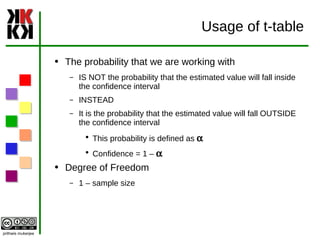
Download as ODP, PPTX
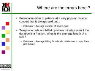
![Why Estimation ? [ From ] Inference For a given population Various statistical parameters are GIVEN or KNOWN Mean, Standard Deviation etc Task was to interpret them and take managerial decisions How many shirts to be stocked in the store ? Is the machine setup faulty ? Should we fix it [ To ] Estimation For the given population or sample Various statistical parameters are NOT KNOWN So managerial decisions cannot be taken UNLESS we can estimate the parameters](https://image.slidesharecdn.com/qt1-07-estimation-090919072536-phpapp01/85/QT1-07-Estimation-2-320.jpg)
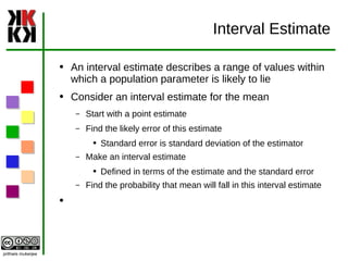

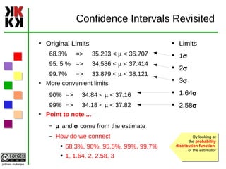
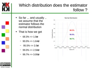
![How do we get this interval [Usually] we are trying to estimate the population mean m We have an estimator E which [ in most cases ] is the sample mean. E follows a distribution that has mean m and standard error s We create a statistic Q = (E – m )/ s Q follows a some distribution ( normal ? T ? ) We identify two values Q 1 , Q 2 such that probability of Q falling between Q 1 and Q 2 is equal to required confidence P Interval is E – Q 1 s < m < E + Q 2 s](https://image.slidesharecdn.com/qt1-07-estimation-090919072536-phpapp01/85/QT1-07-Estimation-20-320.jpg)
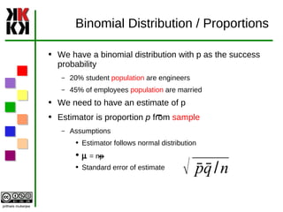
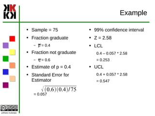

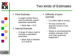
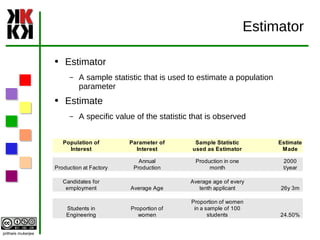
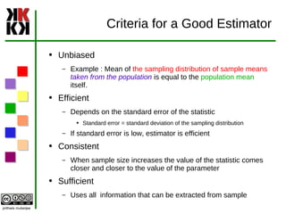
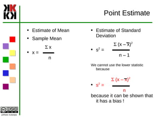
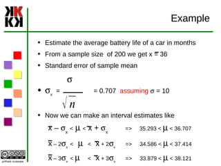
The document discusses estimation and different types of estimates used to estimate population parameters based on sample data. Point estimates provide a single value while interval estimates provide a range of values. Good estimators are unbiased, efficient, and consistent. Common point estimators are the sample mean and sample standard deviation. Interval estimates use the point estimate plus/minus a margin of error calculated from the standard error. Confidence intervals provide a probability that the population parameter lies within the interval estimate.