Introduction to Statistics for schools and colleges.

1. Review of Basic Statistics

2. Definitions
• Population - The set of all items of interest in a
statistical problem
e.g. - Houses in Sacramento
• Parameter - A descriptive measure of a population
e.g. - Mean (average) appraised value of all houses
• Sample - A set of items drawn from a population
e.g. - 100 randomly selected homes
• Statistic - A descriptive measure of a sample
e.g. - Mean appraised value of selected homes
• Statistical inference - The process of making an
estimate, prediction, or decision based upon sample data

3. Types of Data
• Qualitative - Categorical, i.e., data represents
categories
e.g. - Existence of an attached garage
• Quantitative - Data are numerical values
Discrete(countable) - Counts of things
e.g. - Number of bedrooms
Continuous(interval) - Measurements
e.g. - Appraised value or square footage

4. • Cross-sectional - Observations in a sample
are collected at the same time.
e.g. - Our sample of 100 homes; most
surveys
• Time series - Data is collected at successive
points in time
e.g. - Housing starts, recorded monthly
from July 1985 to June 1997

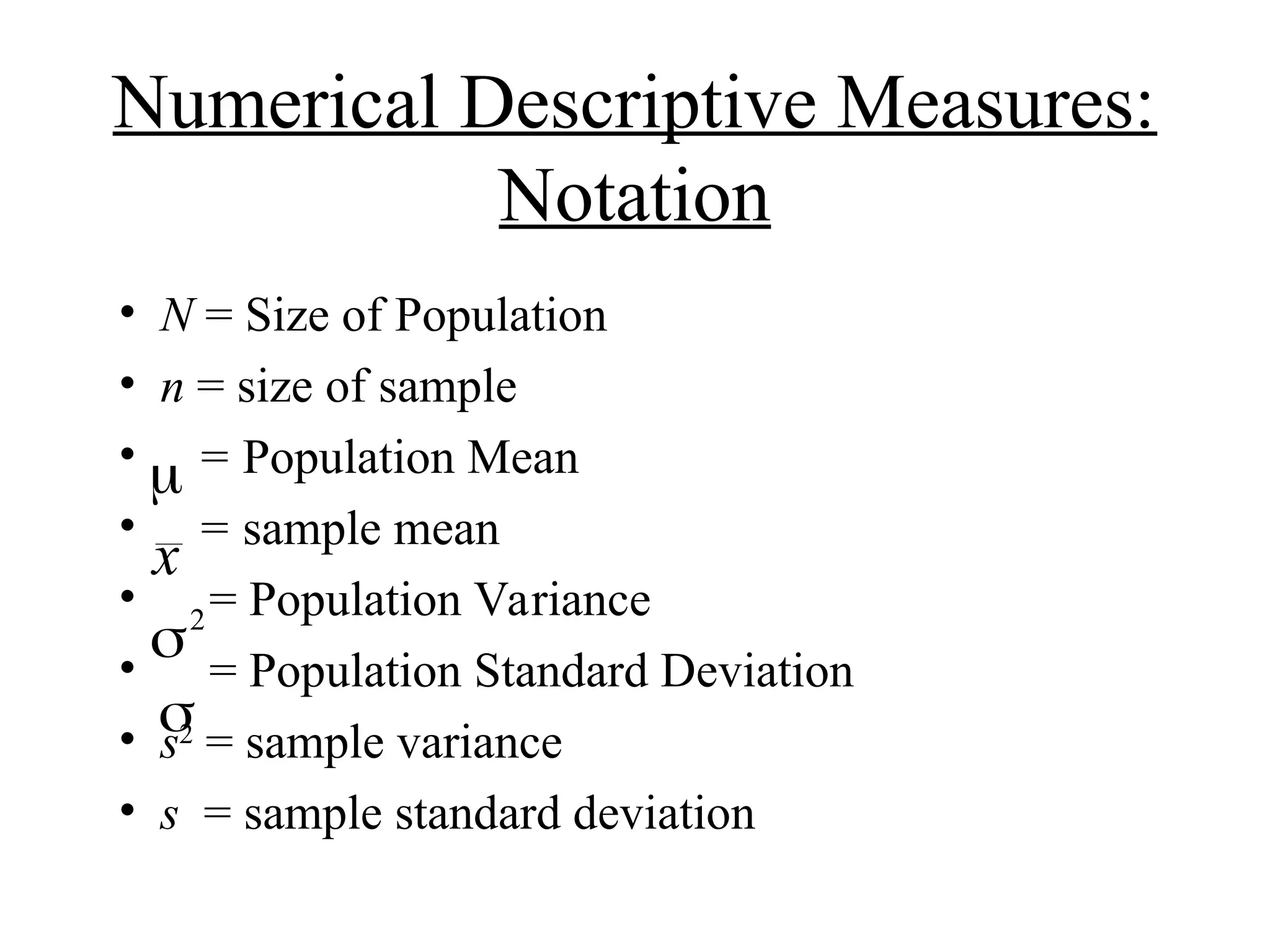
5. Numerical Descriptive Measures:
Notation
• N = Size of Population
• n = size of sample
• = Population Mean
• = sample mean
• = Population Variance
• = Population Standard Deviation
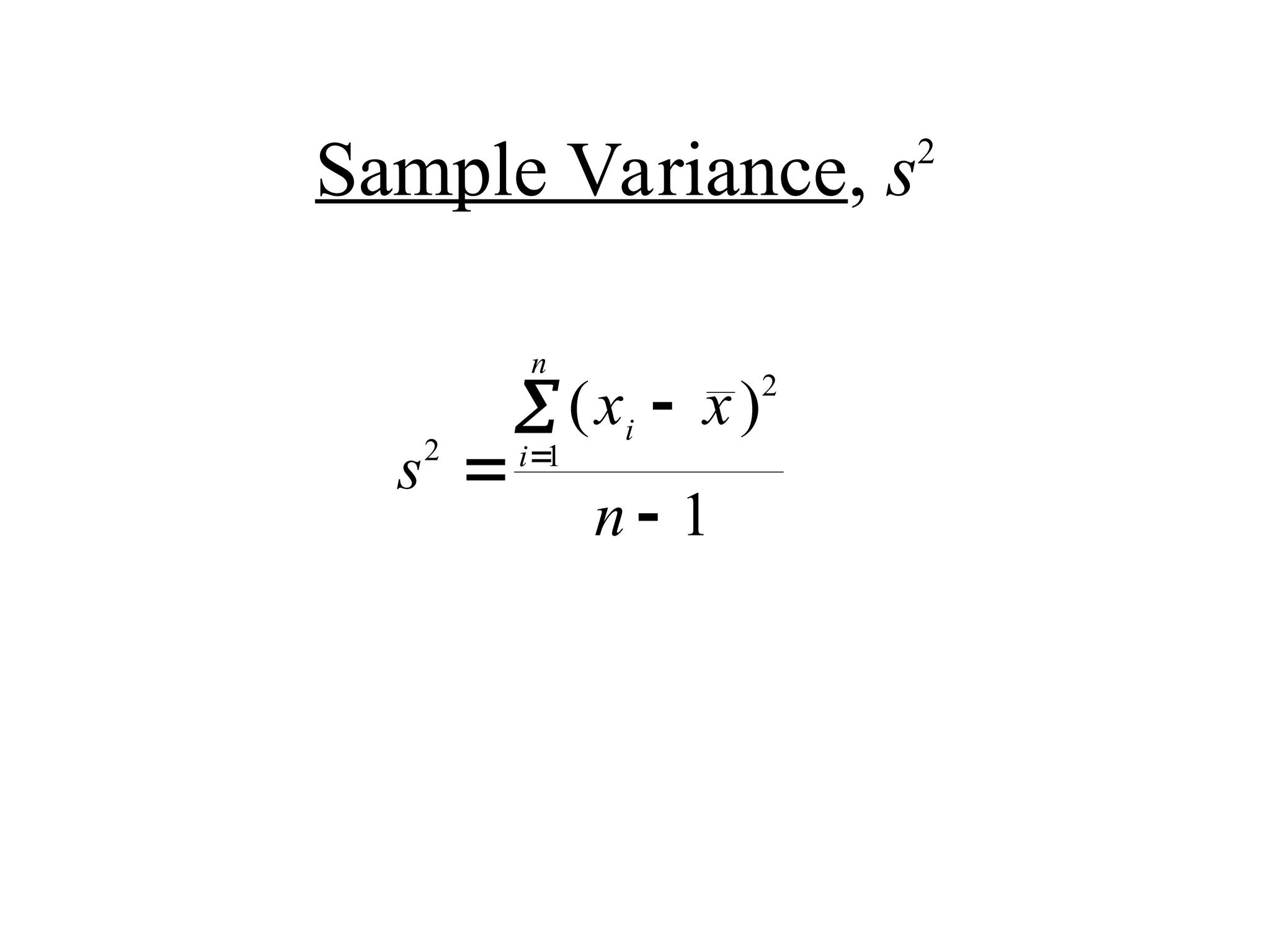
• s2
= sample variance
• s = sample standard deviation
x
2



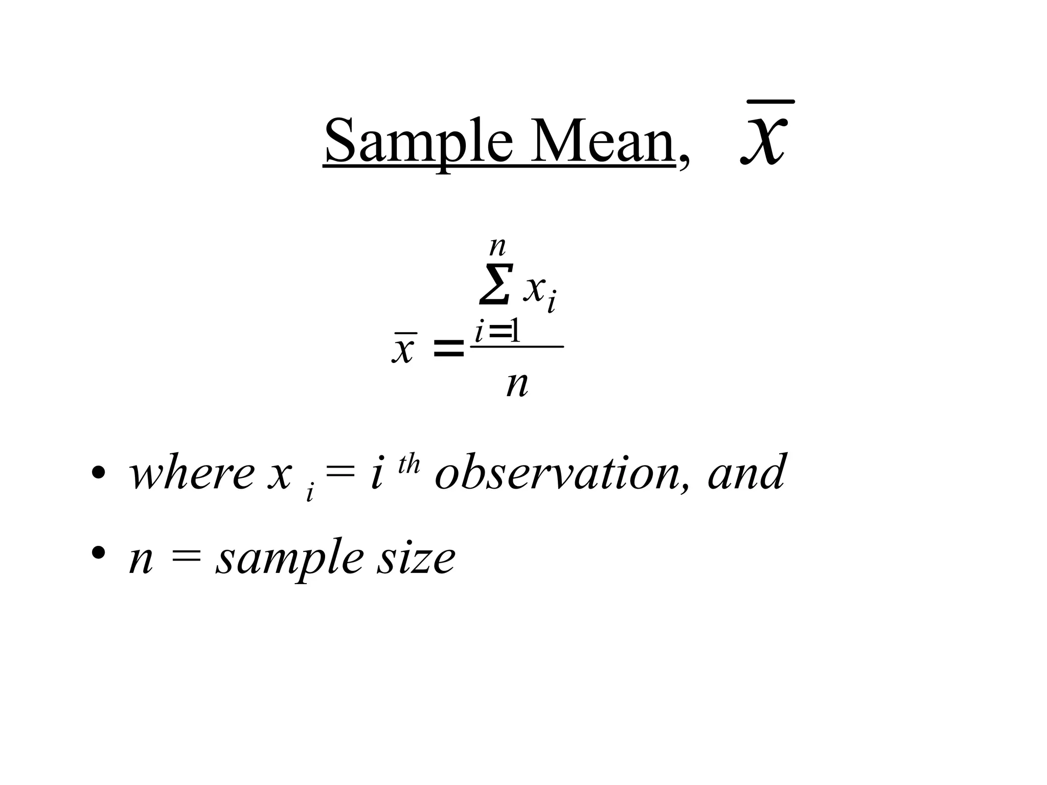
6. Sample Mean,
• where x i = i th
observation, and
• n = sample size
x
x
x
n
i
i
n



1

7. Sample Variance, s2
s
x x
n
i
i
n
2
2
1
1





( )

8. Example
• Find the mean and variance of the following
sample values (in years):
3.4, 2.5, 4.1, 1.2, 2.8, 3.7

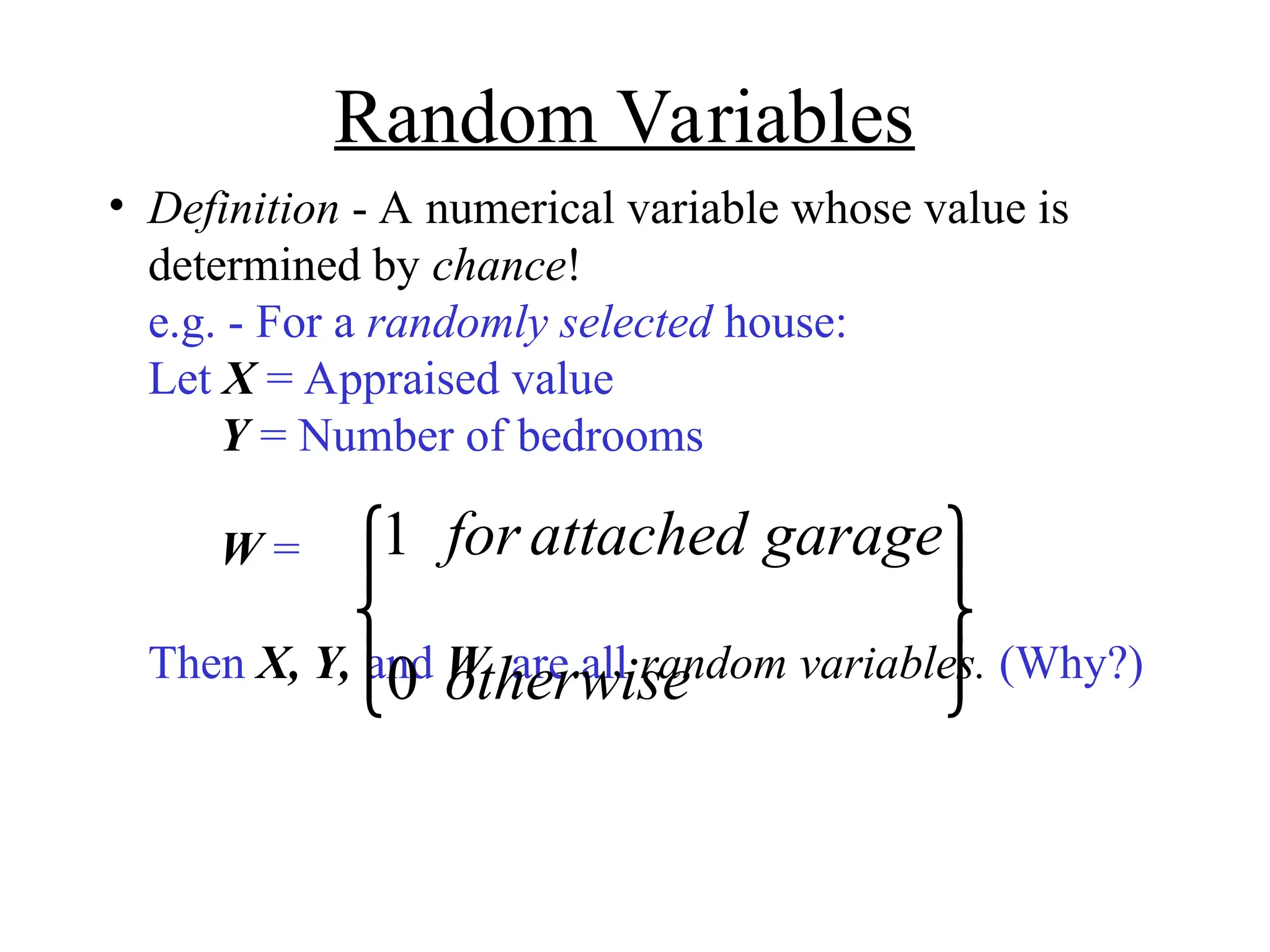
9. Random Variables
• Definition - A numerical variable whose value is
determined by chance!
e.g. - For a randomly selected house:
Let X = Appraised value
Y = Number of bedrooms
W =
Then X, Y, and W are all random variables. (Why?)
1
0
for attached garage
otherwise











10. Note - Let X be a random variable, then
, S2
and S are also random variables
What is the difference between
X, , S2
, S and x, , s2
, s ?
X
X x

11. Probability Distributions
• Definition - A probability distribution for a
random variable describes the values that the
random variable can assume together with the
corresponding probabilities.
• Importance - Its probability distribution describes
the behavior of a random variable. Therefore,
questions concerning a random variable cannot be
answered without reference to its probability
distribution.

12. Mean,
Std. dev.
,
Normal Distributions
X
density
-3 -2 -1  1 2 3
0
0.1
0.2
0.3
0.4

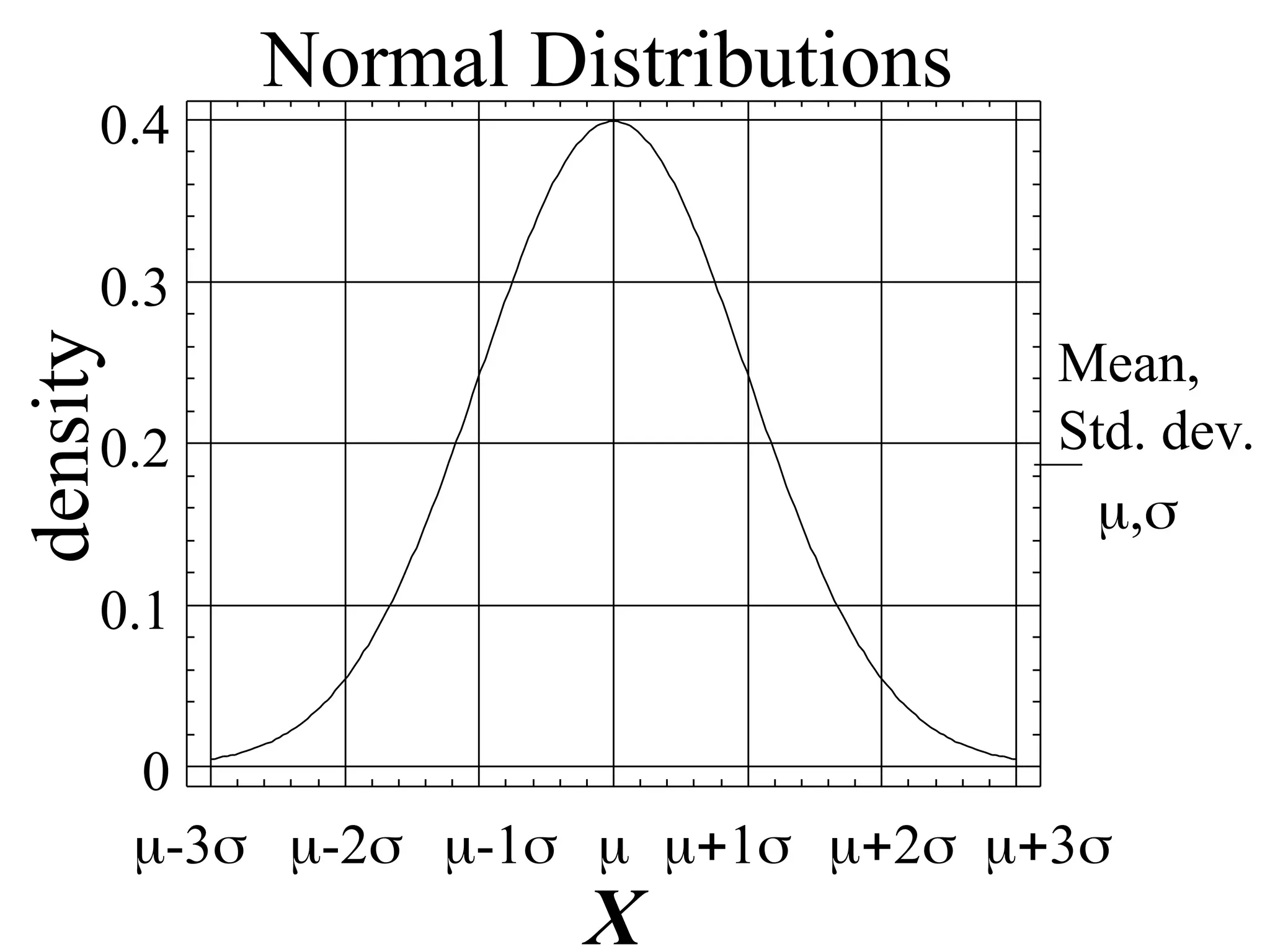
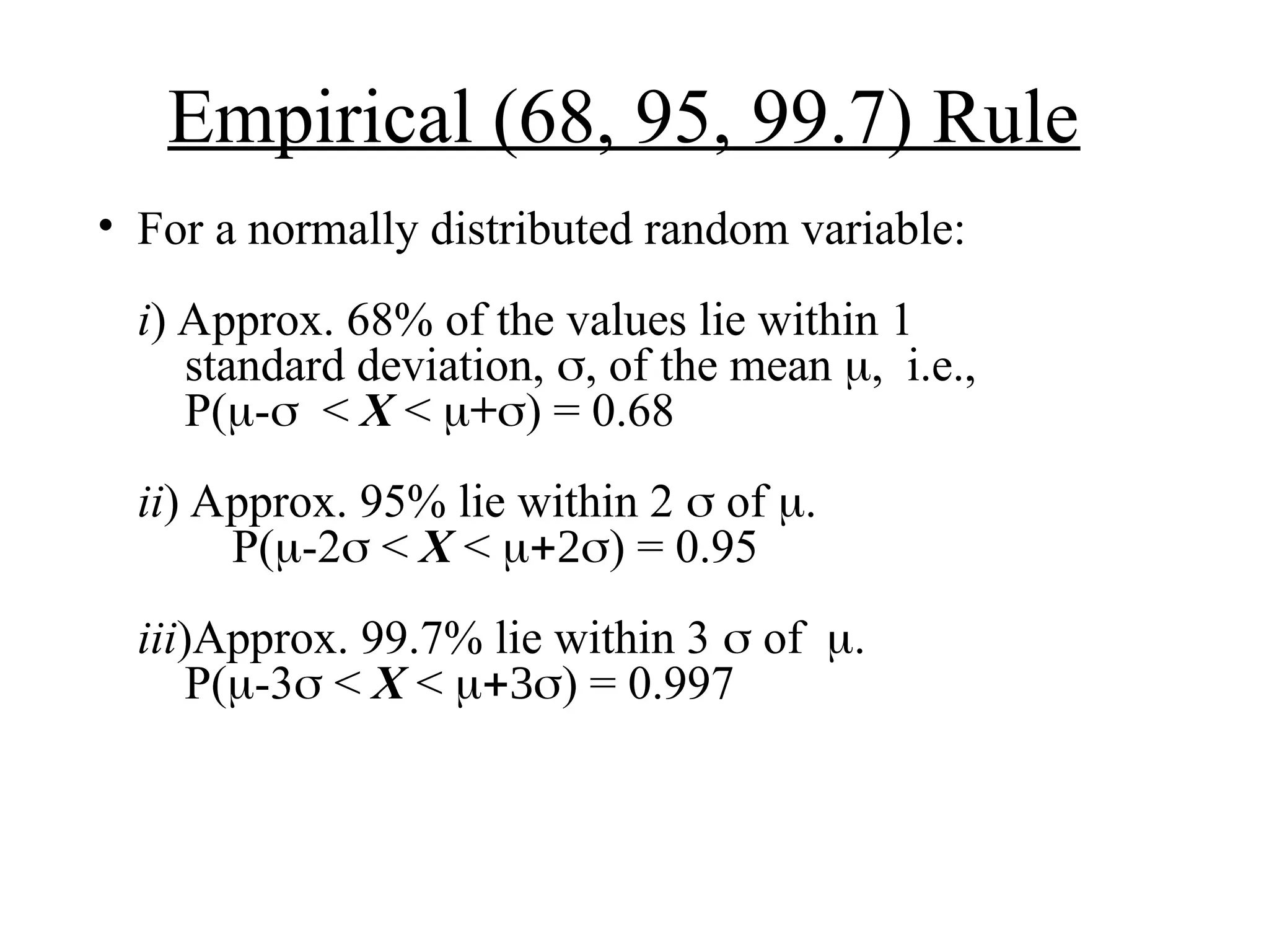
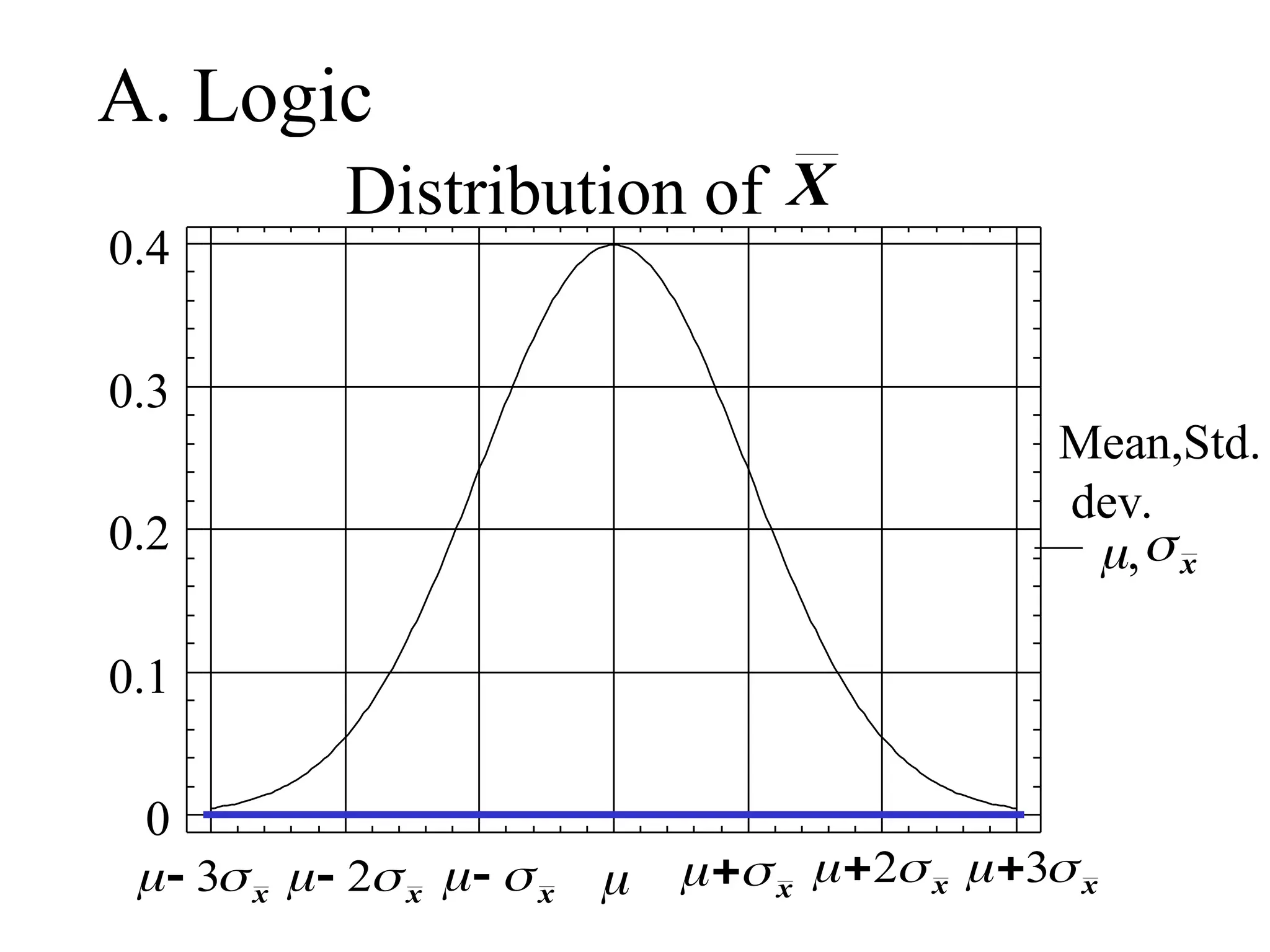
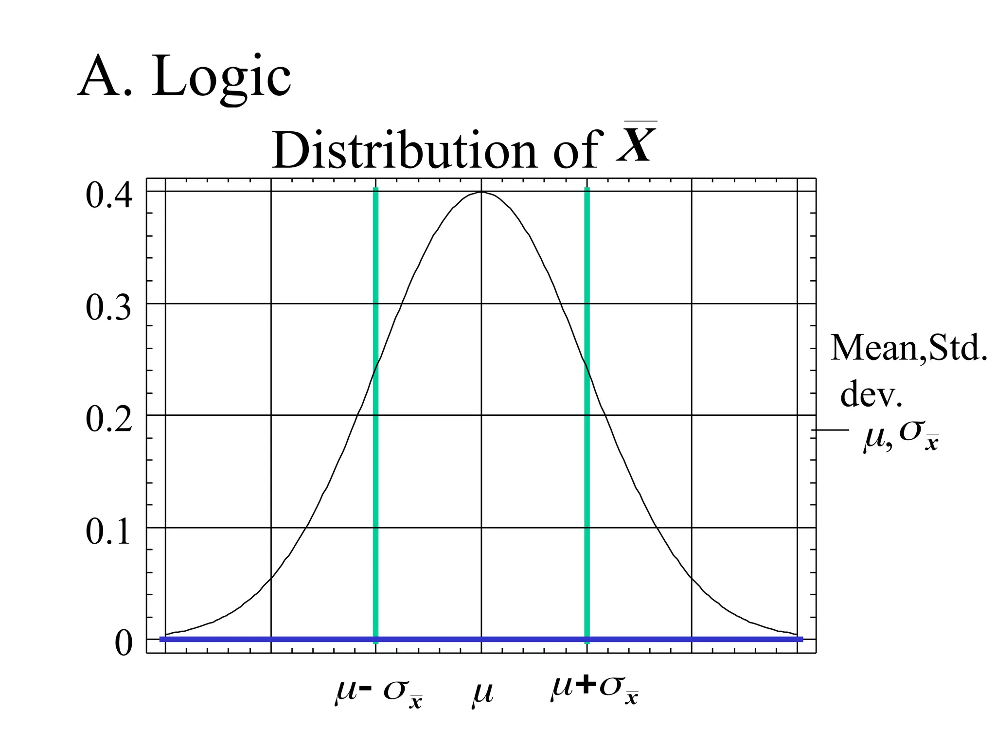
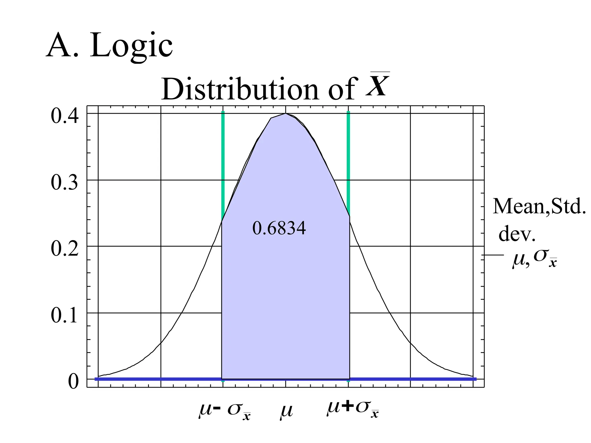
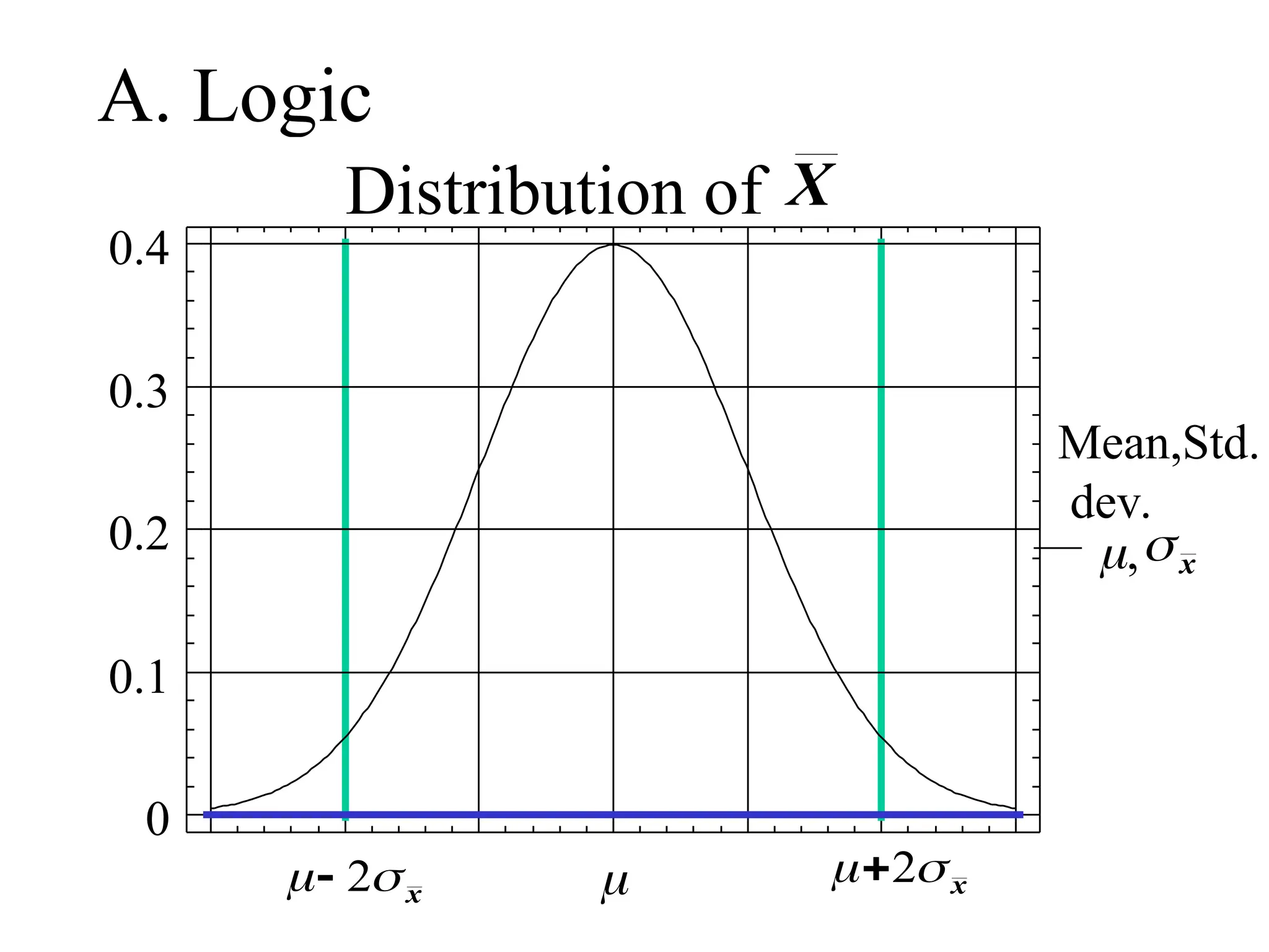
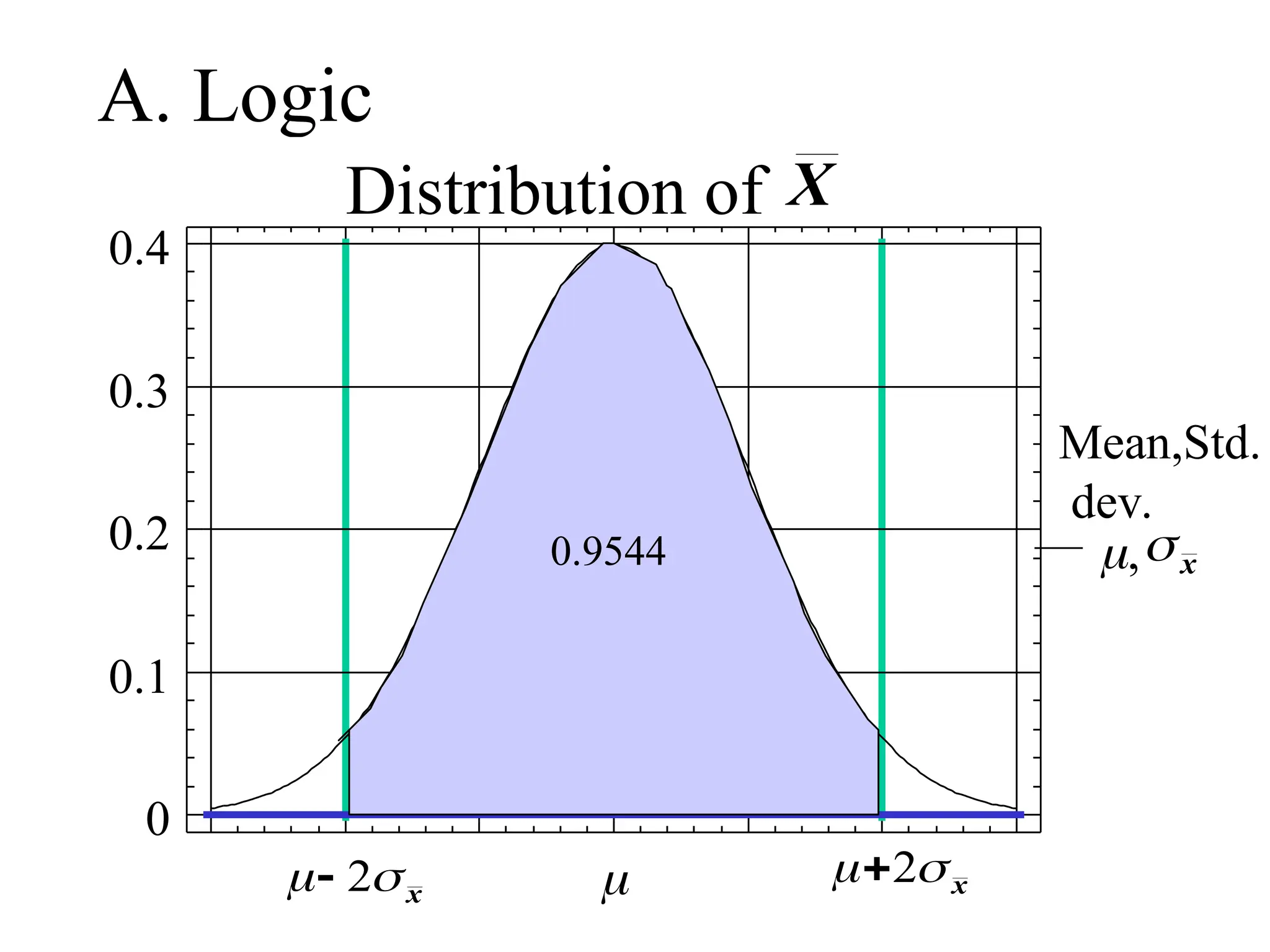
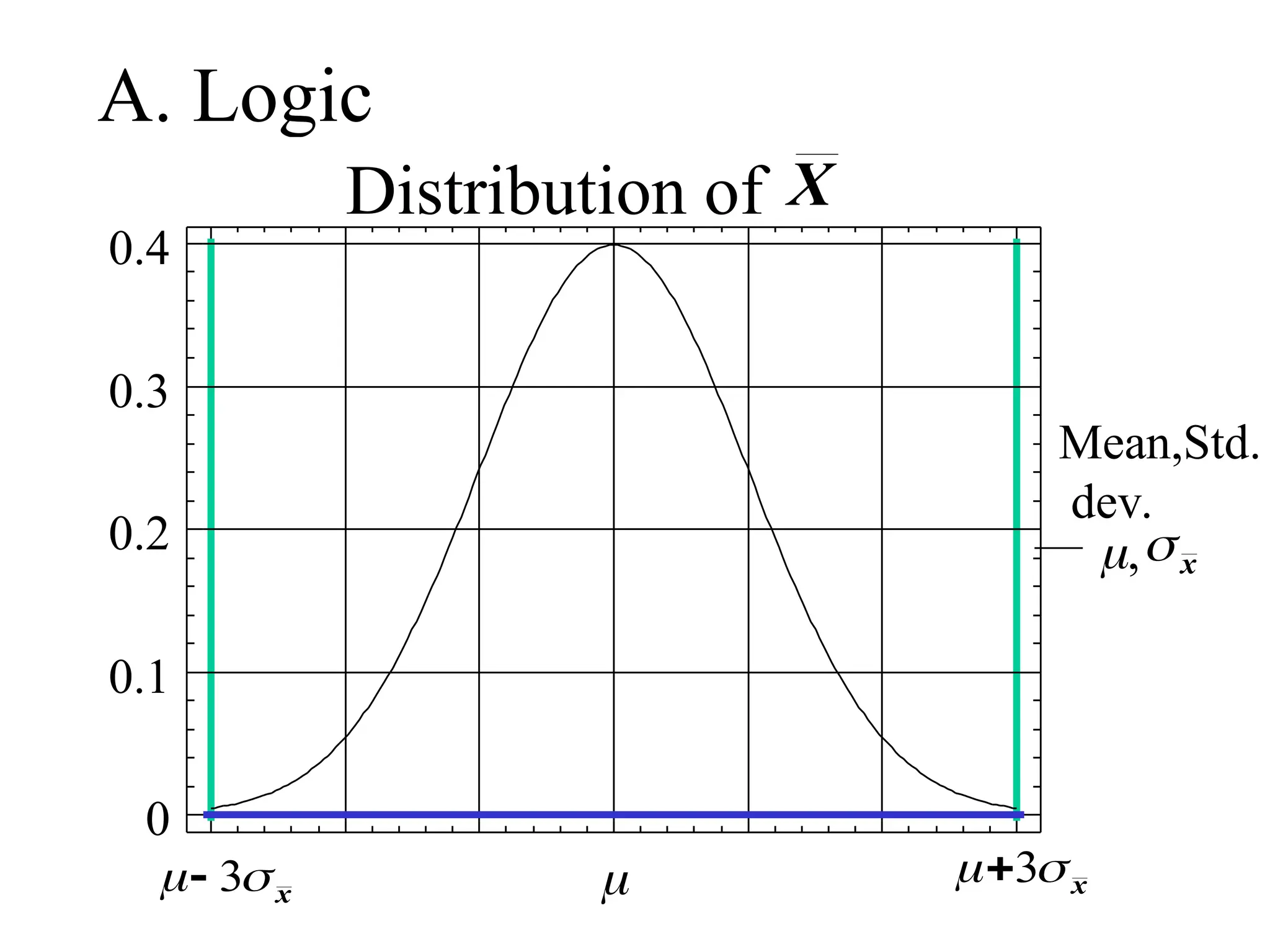
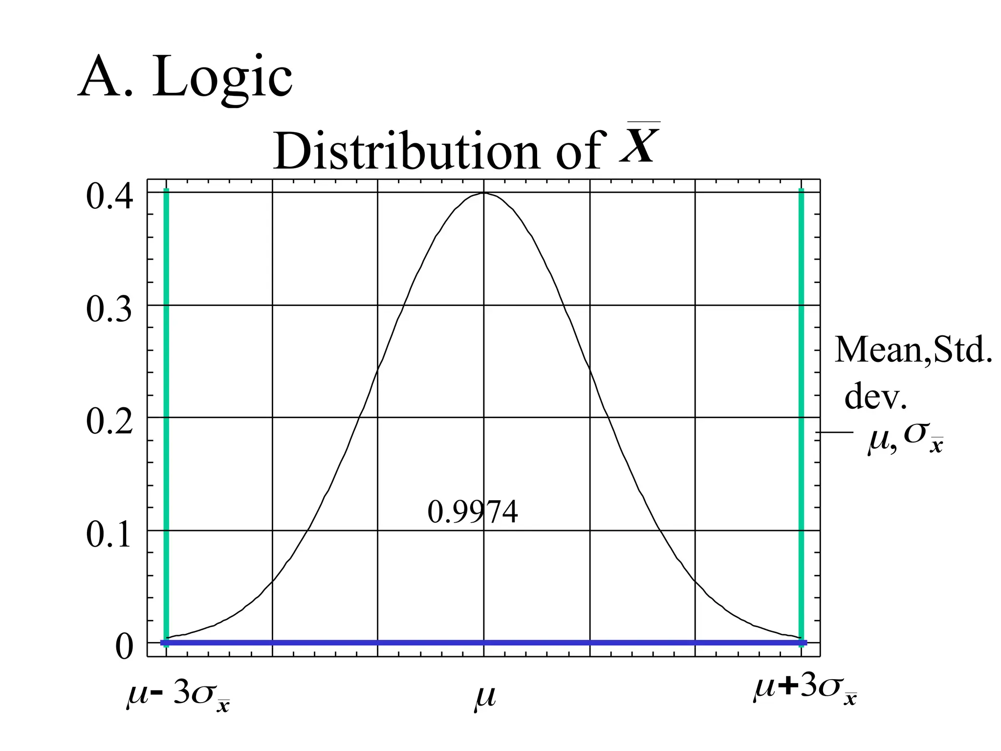
13. Empirical (68, 95, 99.7) Rule
• For a normally distributed random variable:
i) Approx. 68% of the values lie within 1
standard deviation,  of the mean i.e.,
P(-< X < +) = 0.68
ii) Approx. 95% lie within 2  of 
P(-2 < X < ) = 0.95
iii)Approx. 99.7% lie within 3  of.
P(-3 < X < ) = 0.997

14. Standard Normal Distribution
Mean,
Std. dev.
0,
1
Z
density
-3 -2 -1 0 1 2 3
0
0.1
0.2
0.3
0.4

15. Examples
Determine the following:
a. P(0 < Z < 1.46)
b. P(Z > 1.46)
c. P(1.28 < Z <1.46)
d. P(Z < -1.28)

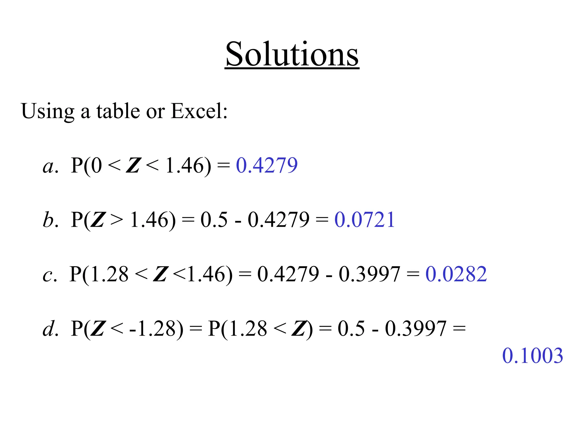
16. Solutions
Using a table or Excel:
a. P(0 < Z < 1.46) = 0.4279
b. P(Z > 1.46) = 0.5 - 0.4279 = 0.0721
c. P(1.28 < Z <1.46) = 0.4279 - 0.3997 = 0.0282
d. P(Z < -1.28) = P(1.28 < Z) = 0.5 - 0.3997 =
0.1003

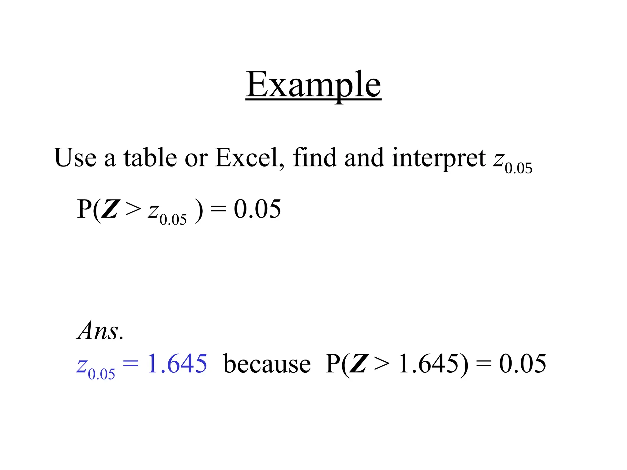
17. Example
Use a table or Excel, find and interpret z
P(Z > z0.05 ) = 0.05
Ans.
z0.05 = 1.645 because P(Z > 1.645) = 0.05

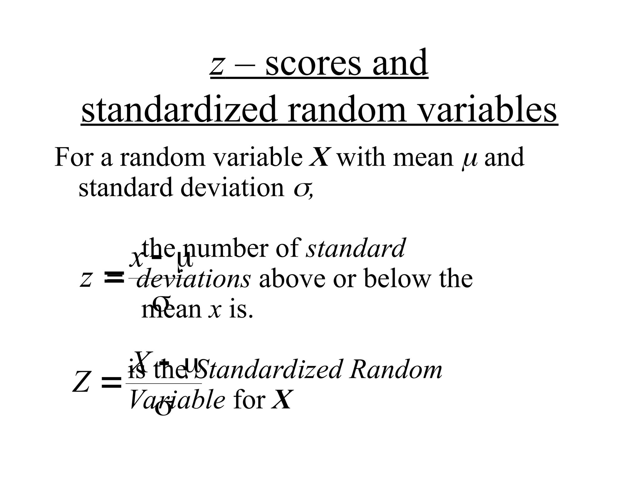
18. z – scores and
standardized random variables
For a random variable X with mean  and
standard deviation ,
the number of standard
= deviations above or below the
mean x is.
is the Standardized Random
Variable for X
z
x

 

Z
X

 


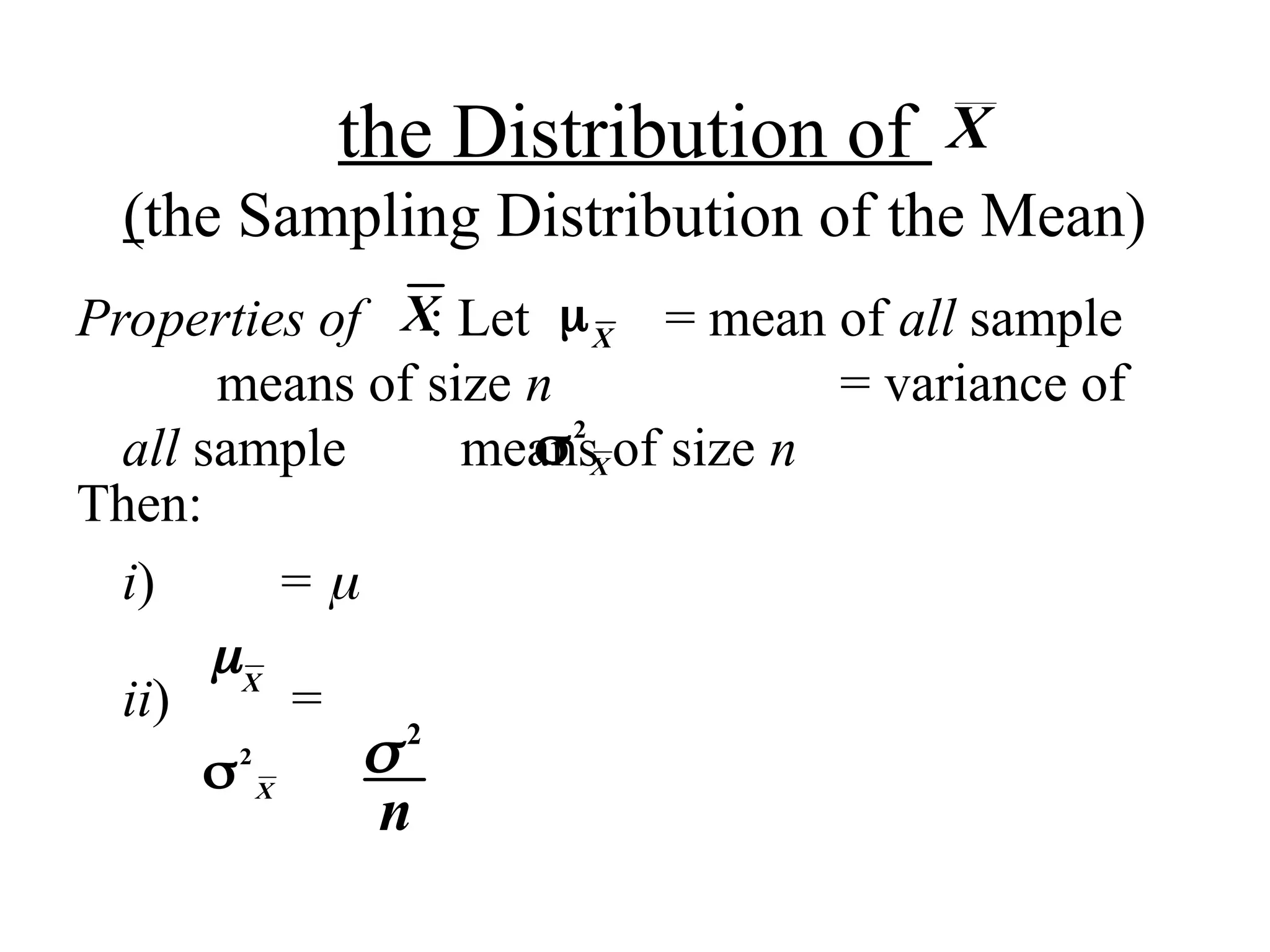
19. the Distribution of
(the Sampling Distribution of the Mean)
Properties of : Let = mean of all sample
means of size n  = variance of
all sample means of size n
Then:
i) = 
ii) =
X
X X
2
X
2
n
X
2
X

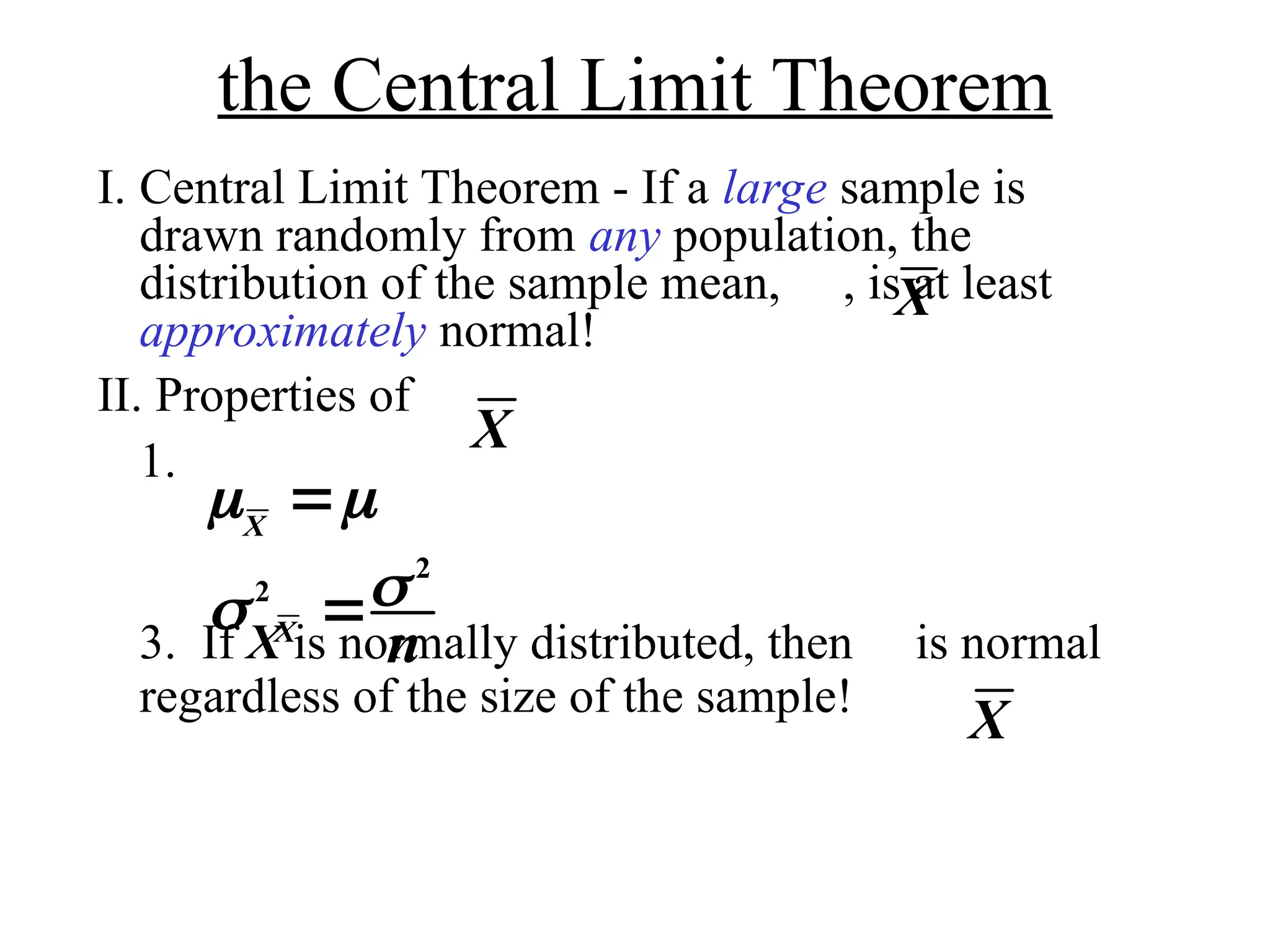
20. the Central Limit Theorem
I. Central Limit Theorem - If a large sample is
drawn randomly from any population, the
distribution of the sample mean, , is at least
approximately normal!
II. Properties of
1.
3. If X is normally distributed, then is normal
regardless of the size of the sample!
X
X
 
X

 
2
2
X
n

X

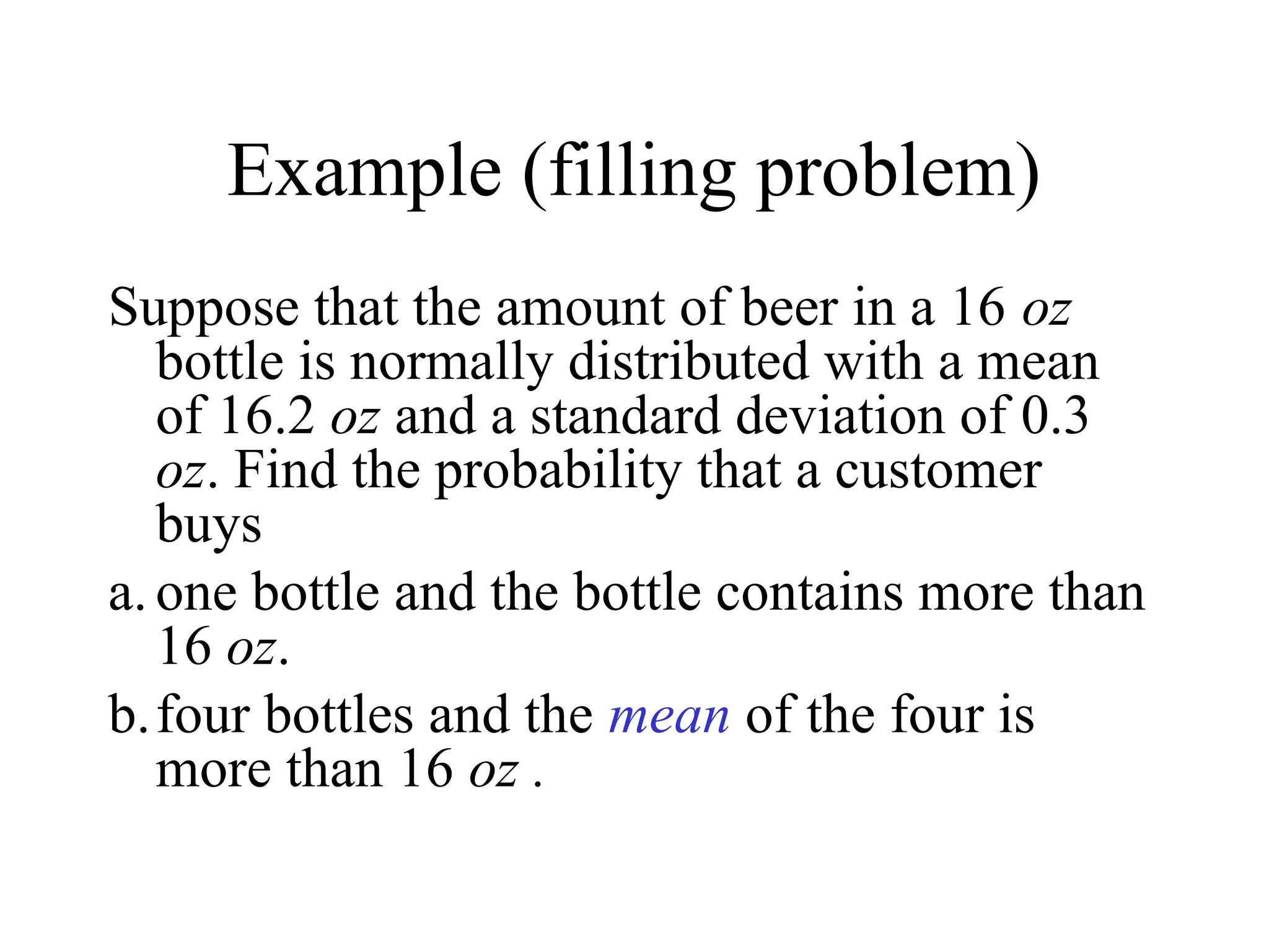
21. Example (filling problem)
Suppose that the amount of beer in a 16 oz
bottle is normally distributed with a mean
of 16.2 oz and a standard deviation of 0.3
oz. Find the probability that a customer
buys
a.one bottle and the bottle contains more than
16 oz.
b.four bottles and the mean of the four is
more than 16 oz .

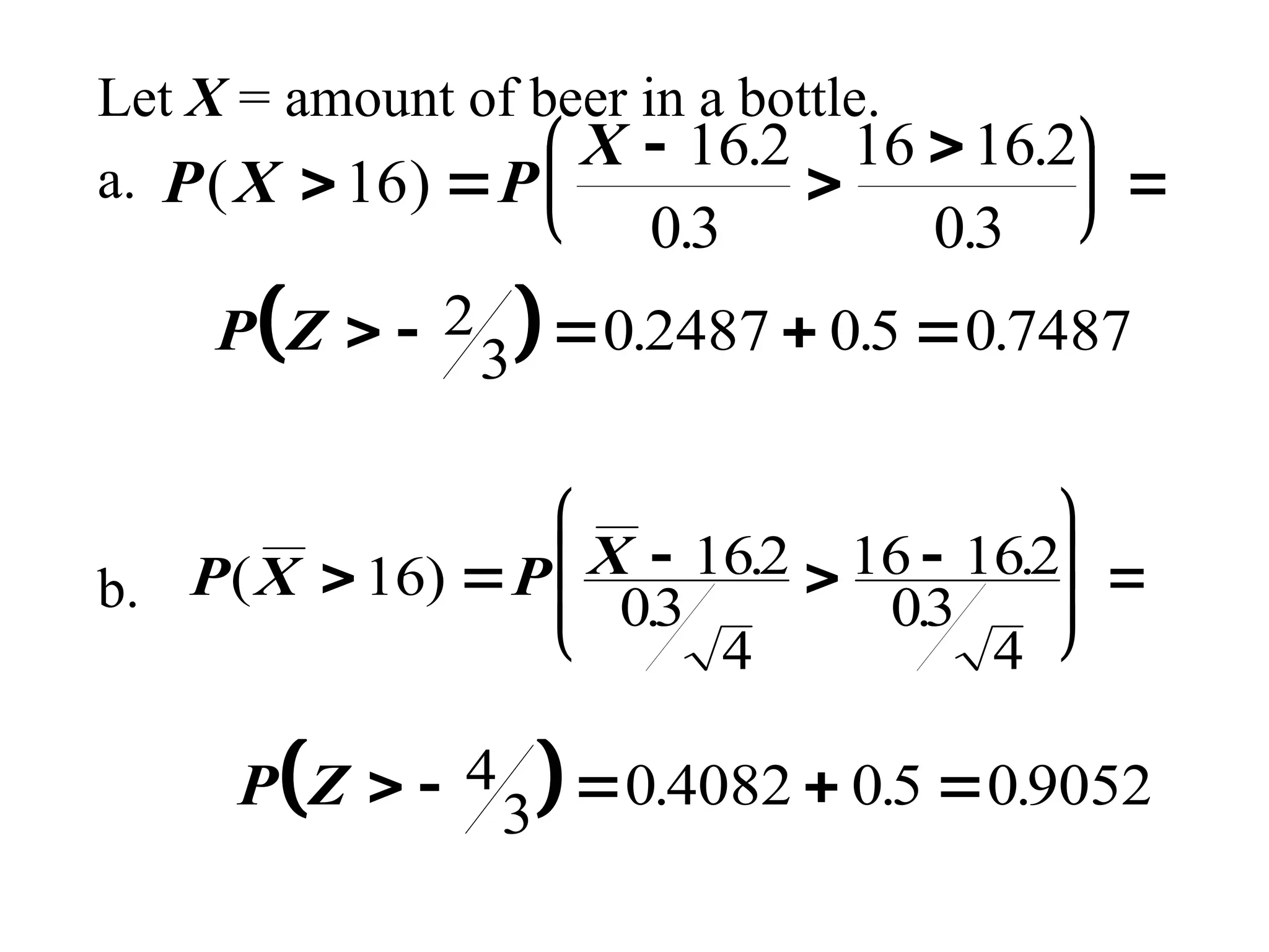
22. Let X = amount of beer in a bottle.
a.
b.
P X P
X
( )
.
.
.
.
 





 

 
16
16 2
03
16 16 2
03
 
P Z     
2
3 0 2487 05 0 7487
. . .
P X P X
( ) .
.
.
.
    









16 162
03
4
16 162
03
4
 
P Z     
4
3 0 4082 05 09052
. . .

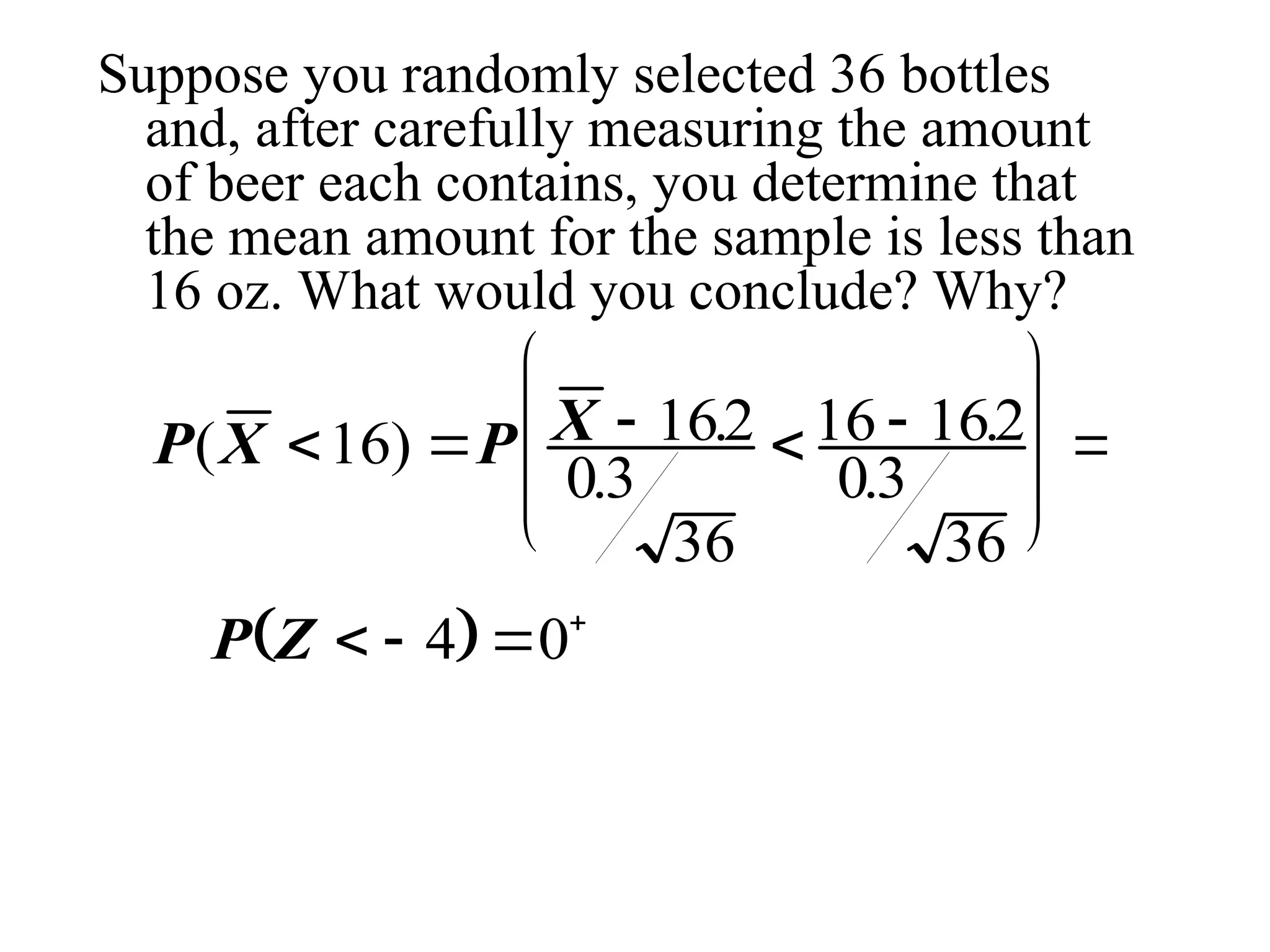
23. Suppose you randomly selected 36 bottles
and, after carefully measuring the amount
of beer each contains, you determine that
the mean amount for the sample is less than
16 oz. What would you conclude? Why?
P X P X
( ) .
.
.
.
    









16 162
03
36
16 162
03
36
 
P Z    
4 0

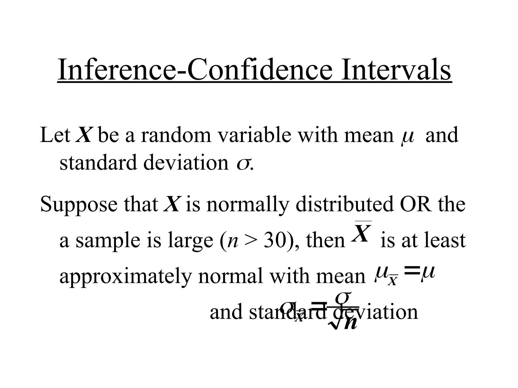
24. Inference-Confidence Intervals
Let X be a random variable with mean and
standard deviation .
Suppose that X is normally distributed OR the
a sample is large (n > 30), then is at least
approximately normal with mean
and standard deviation
X
 
X

 
X
n


25. A. Logic
Mean,Std.
dev.
,
Distribution of

0
0.1
0.2
0.3
0.4
 
 x
 
2 x  
3 x
 
 x
 
 2 x
 
 3 x
x
X

26. A. Logic
Mean,Std.
dev.
,
Distribution of

0
0.1
0.2
0.3
0.4
 
 x
 
 x
x
X

27. A. Logic
Mean,Std.
dev.
,
Distribution of

0
0.1
0.2
0.3
0.4
 
 x
 
 x
x
X
0.6834

28. A. Logic
Mean,Std.
dev.
,
Distribution of

0
0.1
0.2
0.3
0.4
 
2 x
 
 2 x
x
X

29. A. Logic
Mean,Std.
dev.
,
Distribution of

0
0.1
0.2
0.3
0.4
 
2 x
 
 2 x
x
X
0.9544

30. A. Logic
Mean,Std.
dev.
,
Distribution of

0
0.1
0.2
0.3
0.4
 
3 x
 
 3 x
x
X

31. A. Logic
Mean,Std.
dev.
,
Distribution of

0
0.1
0.2
0.3
0.4
 
3 x
 
 3 x
x
X
0.9974

32. A. Logic
Mean,Std.
dev.
,
Distribution of

0
0.1
0.2
0.3
0.4
x
X
Area = 1 -

Area = /2
Area = /2
z
2
 z
2

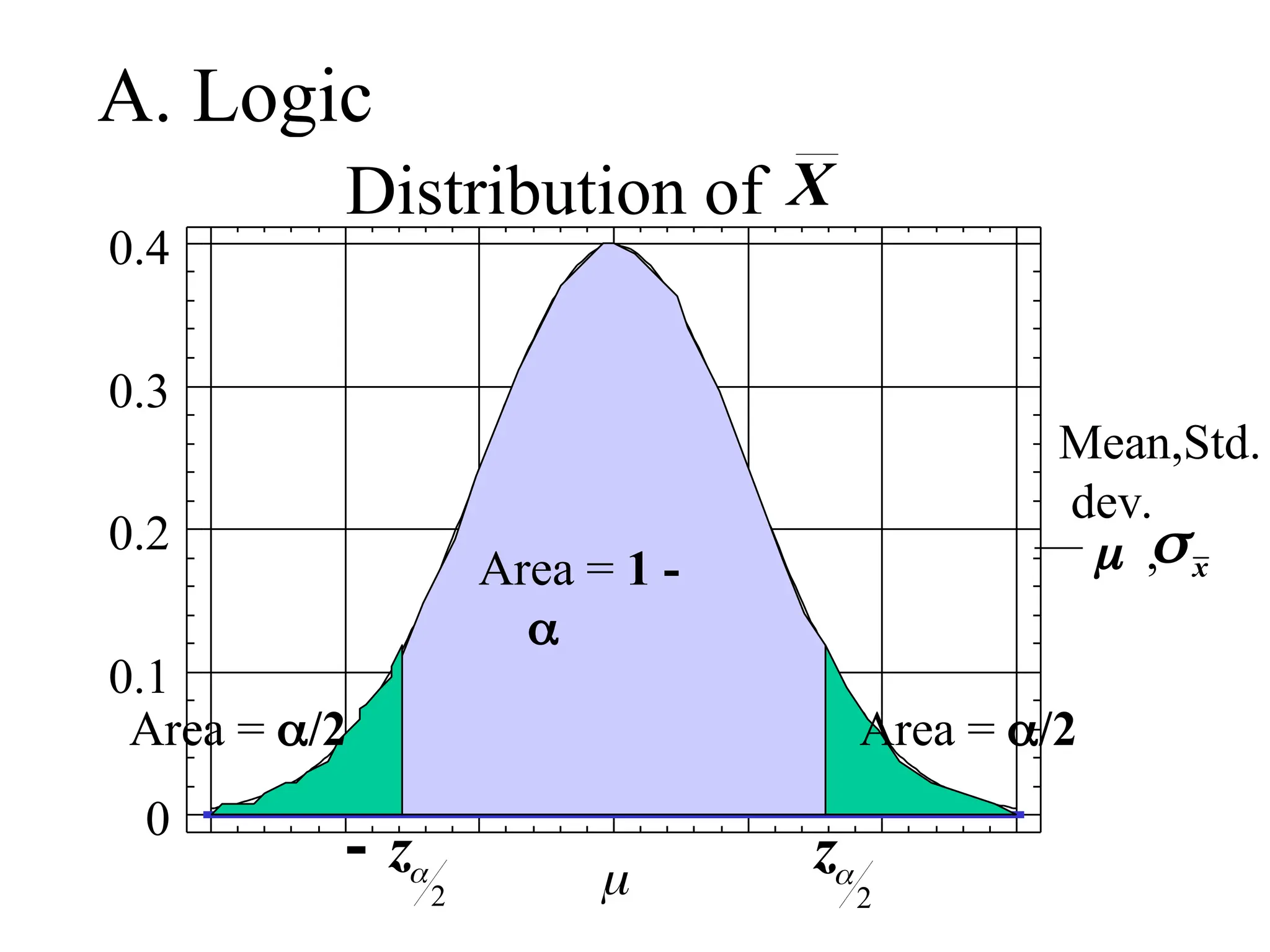
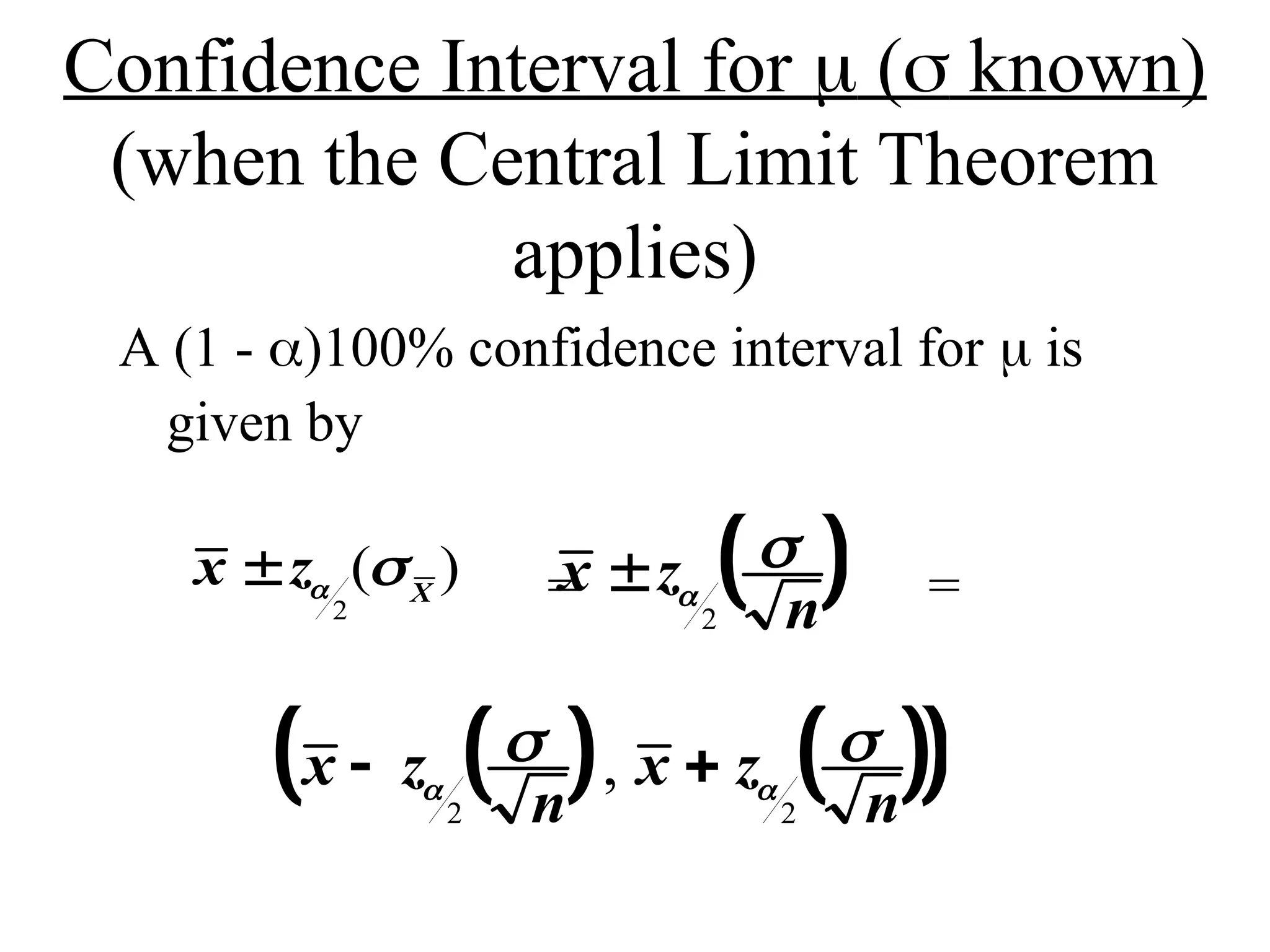
33. Confidence Interval for  ( known)
(when the Central Limit Theorem
applies)
A (1 - )100% confidence interval for  is
given by
= =
 
x z
n
 

2
x z X
  
2
( )
   
 
x z
n
x z
n
 
 
 
2 2
,

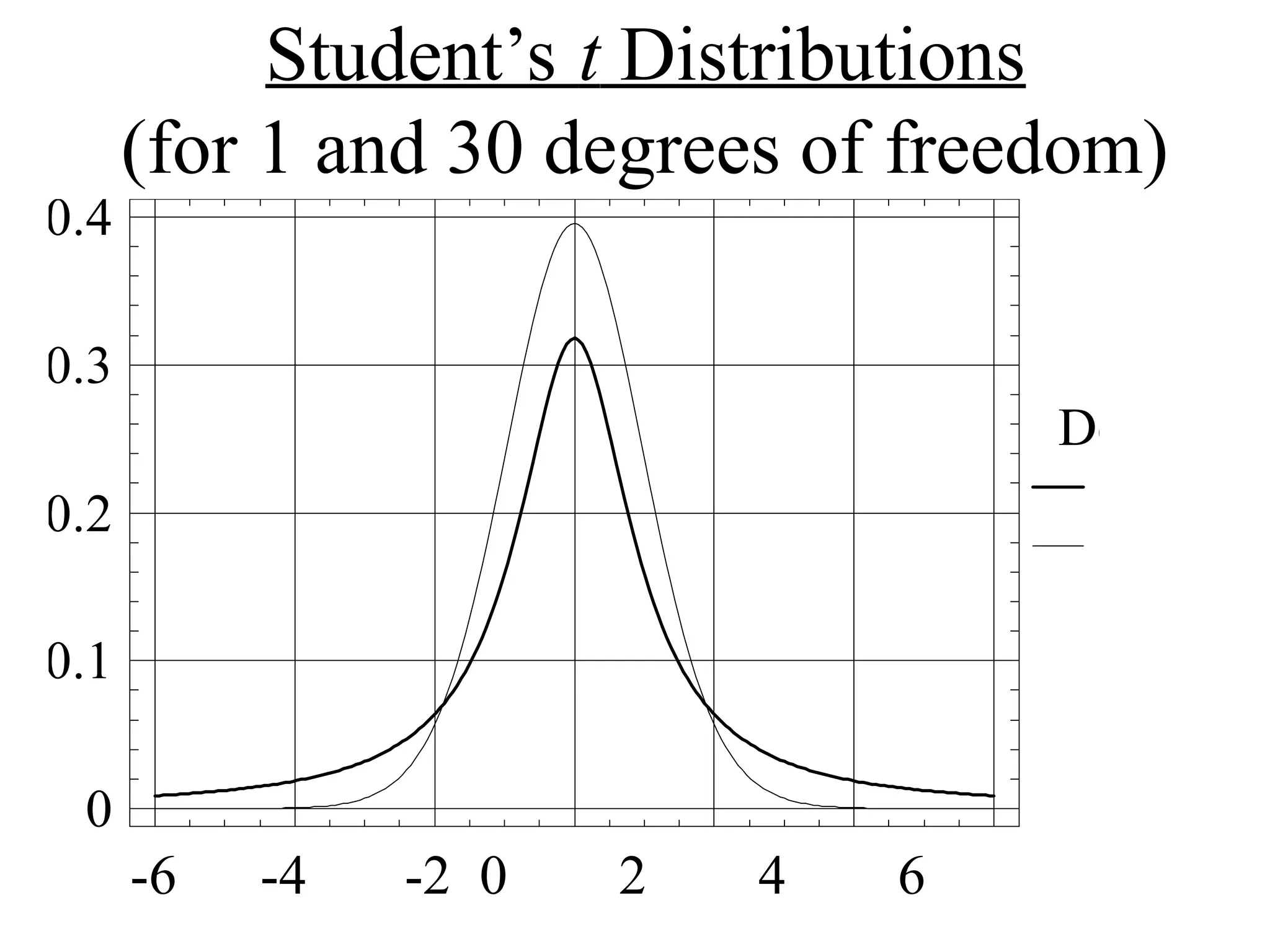
34. Student’s t Distributions
(for 1 and 30 degrees of freedom)
1
30
-6 -4 -2 0 2 4 6
Deg. of fr
1
30
Student's t Distribution
density
-6 -4 -2 0 2 4 6
0
0.1
0.2
0.3
0.4

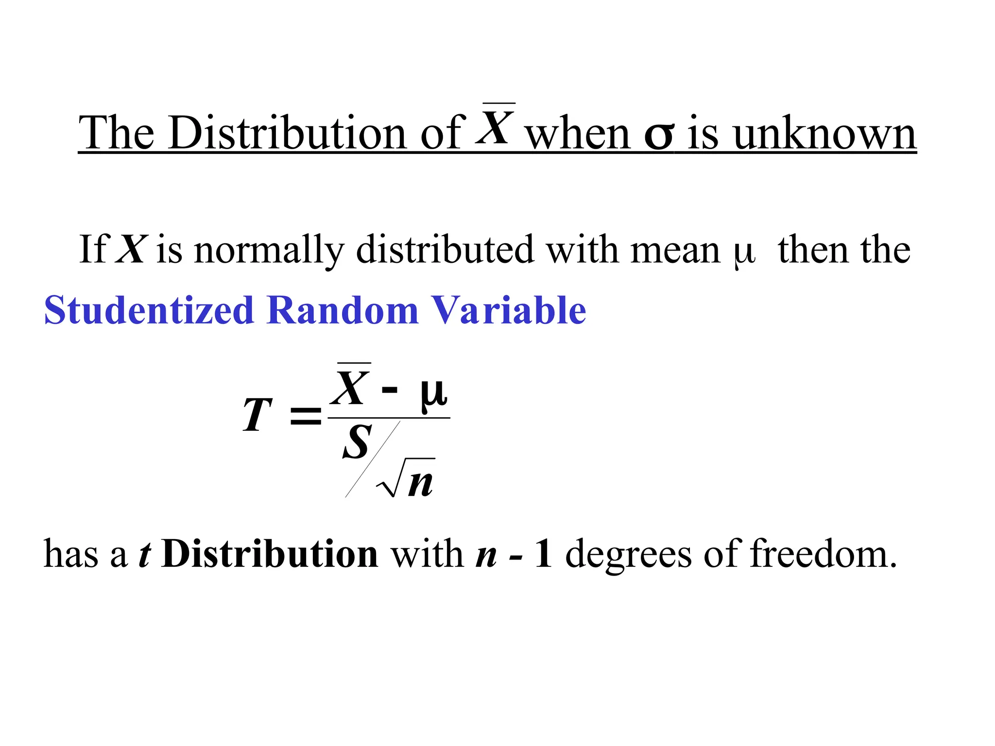
35. The Distribution of when  is unknown
If X is normally distributed with mean then the
Studentized Random Variable
has a t Distribution with n - 1 degrees of freedom.
T
X
S
n

 
X

36. Student's t Distribution
x
density
-4 -3 -2 -1 0 1 2 3 4
0
0.1
0.2
0.3
0.4
df
=
5
Area = 1 - 
Area = 
Area = 
t
2
 t
2

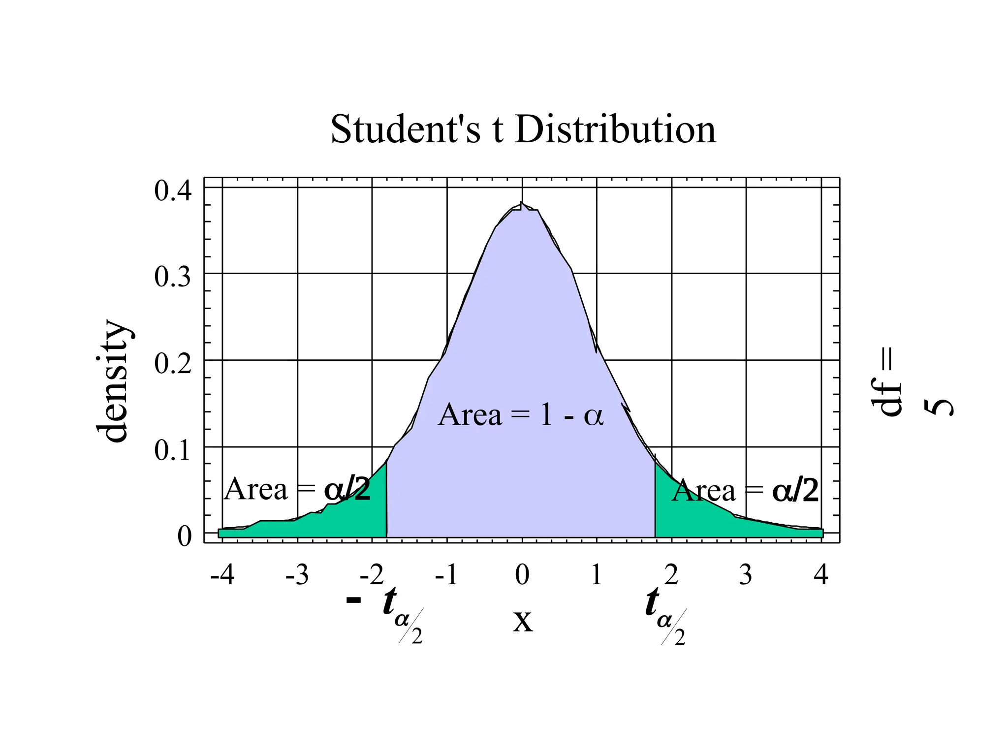
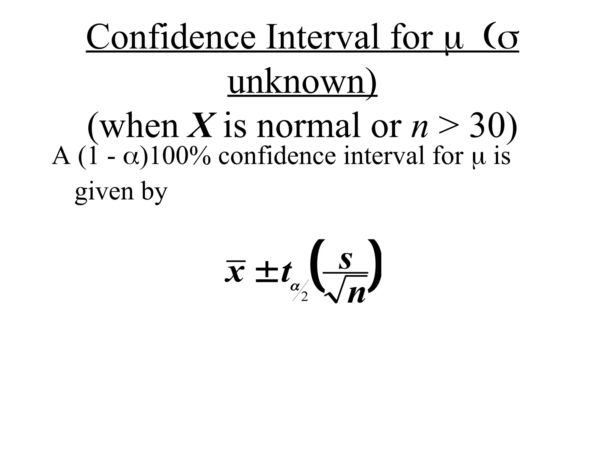
37. Confidence Interval for 
unknown)
(when X is normal or n > 30)
A (1 - )100% confidence interval for  is
given by
 
x t s
n
 
2

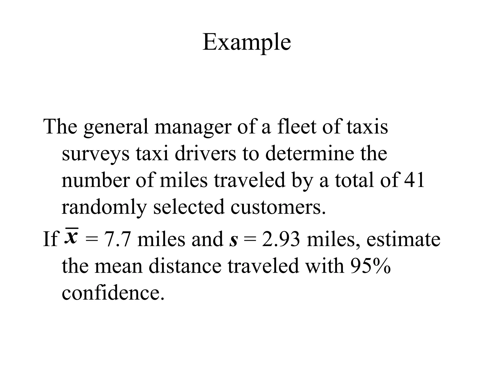
38. Example
The general manager of a fleet of taxis
surveys taxi drivers to determine the
number of miles traveled by a total of 41
randomly selected customers.
If = 7.7 miles and s = 2.93 miles, estimate
the mean distance traveled with 95%
confidence.
x

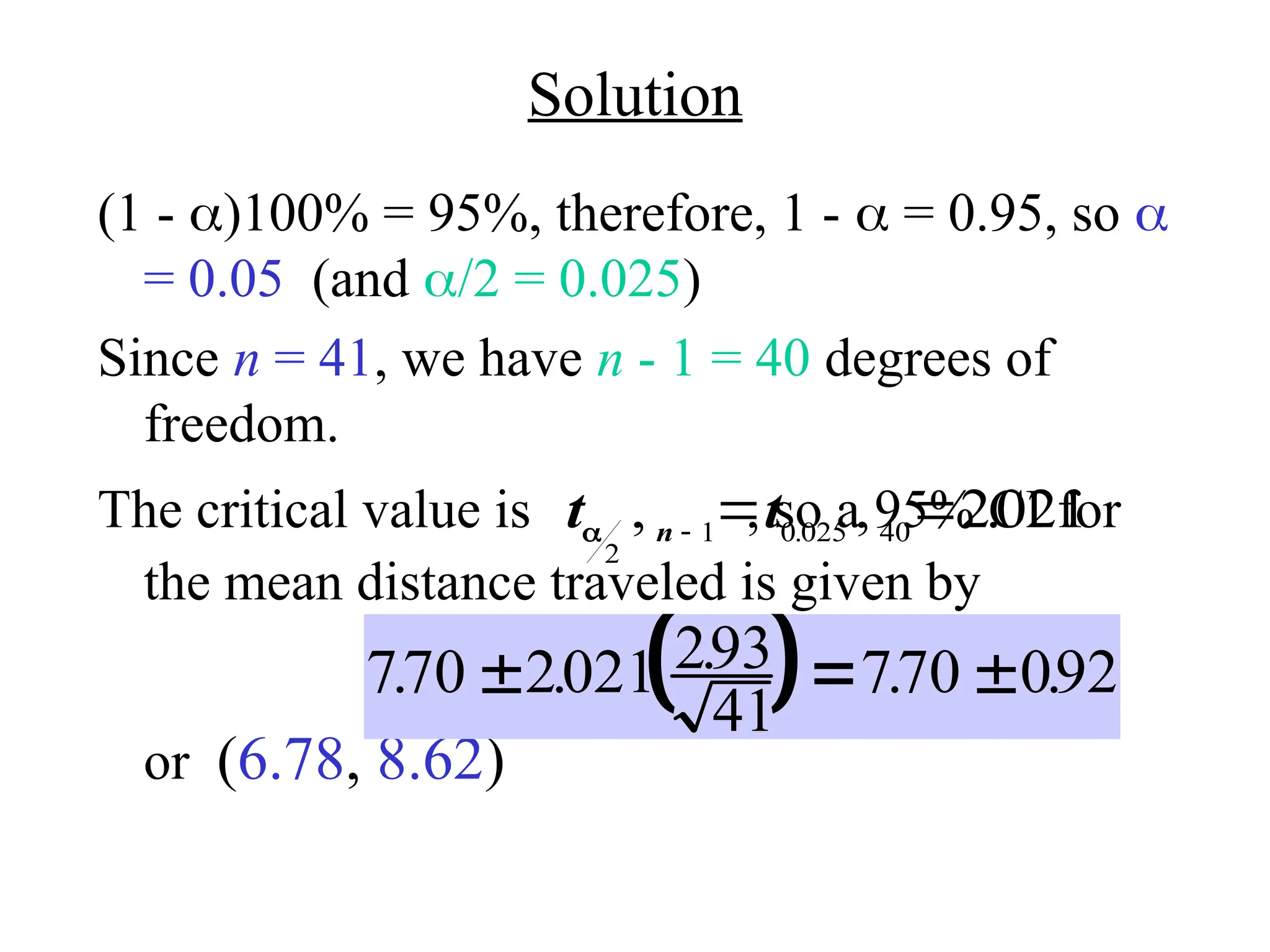
39. Solution
(1 - )100% = 95%, therefore, 1 -  = 0.95, so 
= 0.05 (and /2 = 0.025)
Since n = 41, we have n - 1 = 40 degrees of
freedom.
The critical value is , so a 95% CI for
the mean distance traveled is given by
or (6.78, 8.62)
t t
n

2
1 0 025 40
2021
, , .
.

 
 
770 2021 293
41
770 092
. . . . .
  

40. Hypothesis Tests for( Known)
Assumptions:
• X has mean 
• X is normally distributed OR the sample is
large, i.e., n > 30

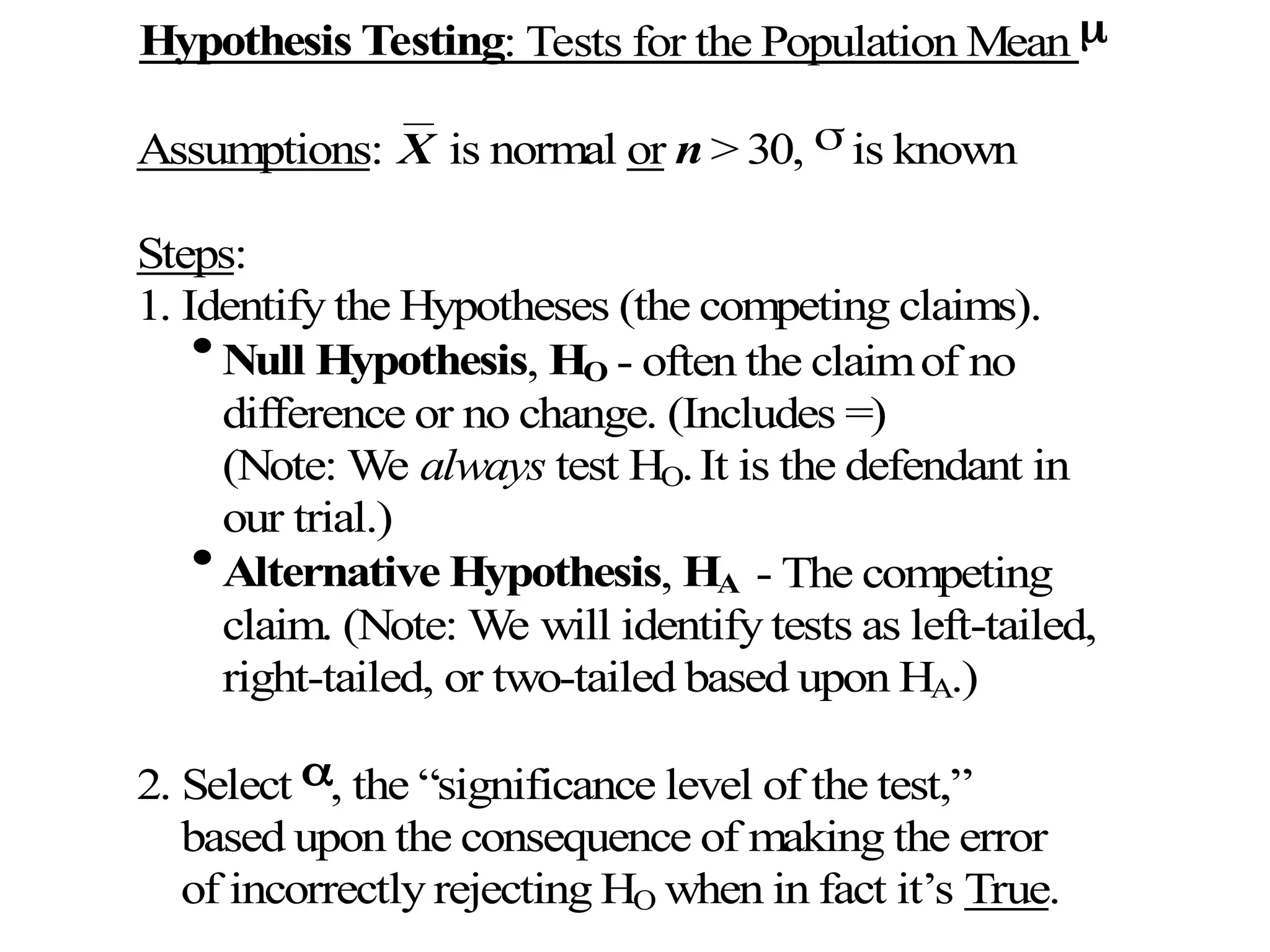
41. Hypothesis Testing: Tests for the Population Mean 
Assumptions: X is normal or n > 30,  is known
Steps:
1. Identify the Hypotheses (the competing claims).

Null Hypothesis, HO - often the claimof no
difference or no change. (Includes =)
(Note: We always test HO.It is the defendant in
our trial.)

Alternative Hypothesis, HA - The competing
claim. (Note: We will identify tests as left-tailed,
right-tailed, or two-tailed based upon HA.)
2. Select , the “significance level of the test,”
based upon the consequence of making the error
of incorrectly rejecting HO when in fact it’s True.

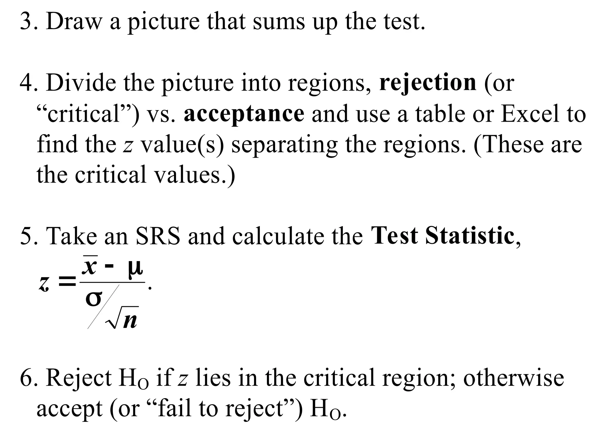
42. 3. Draw a picture that sums up the test.
4. Divide the picture into regions, rejection (or
“critical”) vs. acceptance and use a table or Excel to
find the z value(s) separating the regions. (These are
the critical values.)
5. Take an SRS and calculate the Test Statistic,
z
x
n

 

.
6. Reject HO if z lies in the critical region; otherwise
accept (or “fail to reject”) HO.

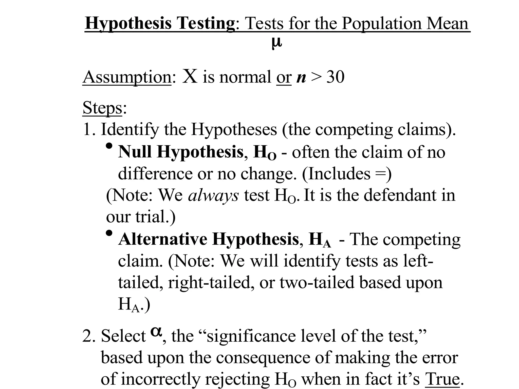
43. Hypothesis Testing: Tests for the Population Mean

Assumption: X is normal or n > 30
Steps:
1. Identify the Hypotheses (the competing claims).

Null Hypothesis, HO - often the claim of no
difference or no change. (Includes =)
(Note: We always test HO. It is the defendant in
our trial.)

Alternative Hypothesis, HA - The competing
claim. (Note: We will identify tests as left-
tailed, right-tailed, or two-tailed based upon
HA.)
2. Select , the “significance level of the test,”
based upon the consequence of making the error
of incorrectly rejecting HO when in fact it’s True.

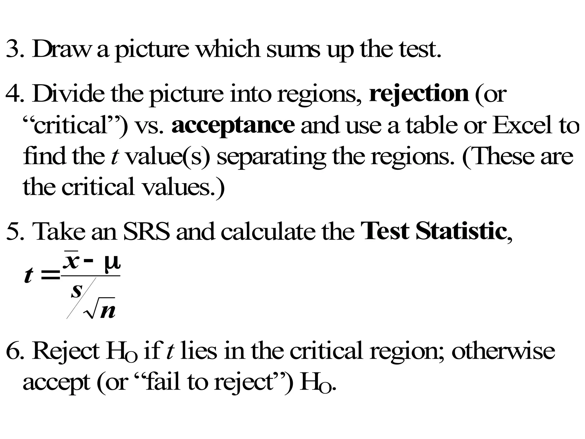
44. 3. Drawa picture which sums up the test.
4. Divide the picture into regions, rejection (or
“critical”) vs. acceptance and use a table or Excel to
find the t value(s) separating the regions. (These are
the critical values.)
5. Take an SRS and calculate the Test Statistic,
t
x
s
n

 
6. Reject HO if t lies in the critical region; otherwise
accept (or “fail to reject”) HO.

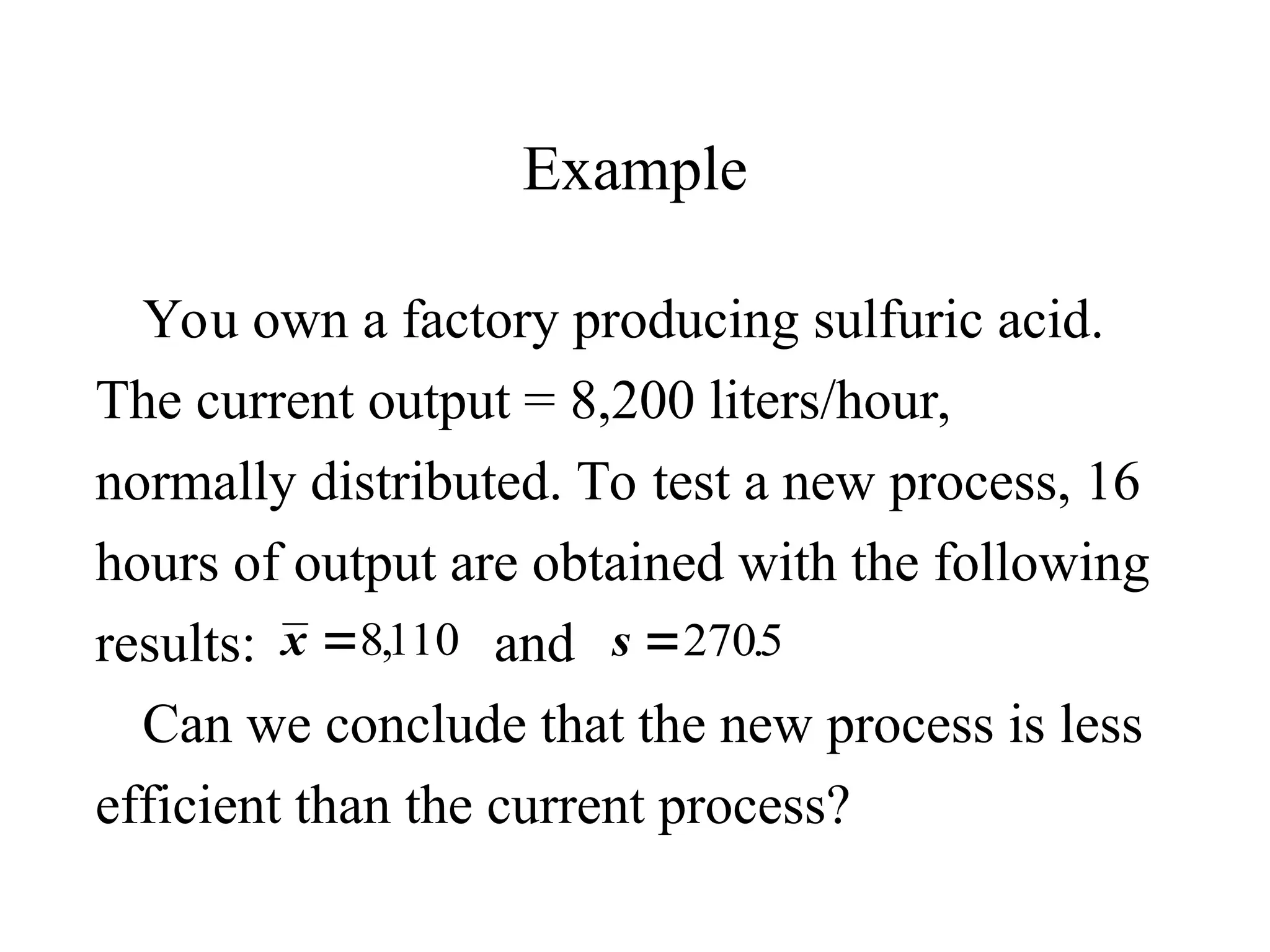
45. Example
You own a factory producing sulfuric acid.
The current output = 8,200 liters/hour,
normally distributed. To test a new process, 16
hours of output are obtained with the following
results: and
Can we conclude that the new process is less
efficient than the current process?
x 8110
, s 2705
.

46. P - Values (Probability Values)
Definition - The p-value is the smallest
significance level at which you would reject
Ho. (the p-value represents a tail probability.)
Using p-values in Hypothesis Tests:
• If p-value < , then Reject Ho
• If p-value >, thenaccept (fail to reject) Ho
We reject Ho for small p-values!