Download as PDF, PPTX
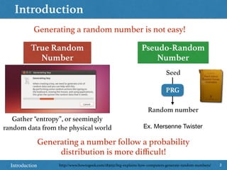


![Standard distributions
11.1 Basic Sampling Algorithms 6
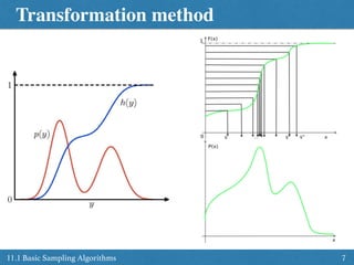
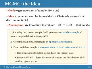
• Goal: Sampling from desired distribution p(y) .
• Assumption: can generate random in U[0,1]
z y = h 1
(z)
h(y) =
Z y
1
p(x)dx
Generate
random
Transform
Uniformly
distributed
h is cumulative
distribution of p
0 y < 1
h(y) = 1 exp( y)
p(y) = exp( y)
y = 1
ln(1 z)
Ex. Consider exponential
distribution
where
then
and
p(y) = p(z)
dz
dy If h-1 is easy to know](https://image.slidesharecdn.com/prmlreadingchapter11samplingmethodver2-160110083330/85/PRML-Reading-Chapter-11-Sampling-Method-6-320.jpg)
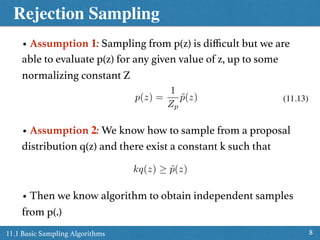
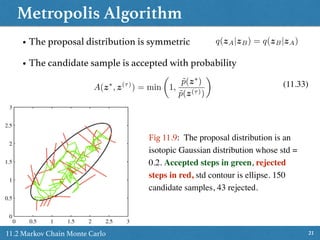
![Rejection Sampling
911.1 Basic Sampling Algorithms
Generate z0
from
proposal
q(.)
Consider
constant k
such that
kq(z) cover
p~(z)
Generate
u0 from
U[0, kq(z0)]
Reject z0 if
Keep z0 if
u0 > ˜p(z0)
u0 ˜p(z0)
• Efficiency of the method
depend on the ratio between
the grey area and the white
area
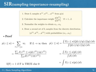
• Proof p(accept) =
Z
˜p(z)
kq(z)
q(z)dz
=
1
k
Z
˜p(z)dz](https://image.slidesharecdn.com/prmlreadingchapter11samplingmethodver2-160110083330/85/PRML-Reading-Chapter-11-Sampling-Method-9-320.jpg)
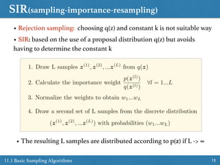
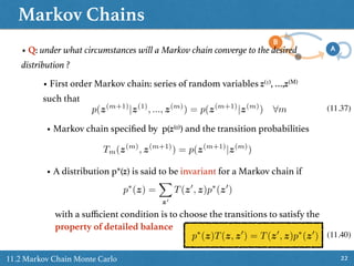
![Rejection Sampling Example
1011.1 Basic Sampling Algorithms
• Sampling from Gamma
distribution (green curve)
Gam(z|a, b) =
ba
za 1
exp( bz)
(a)
at z = (a-1)/b
• Proposal distribution -> Cauchy
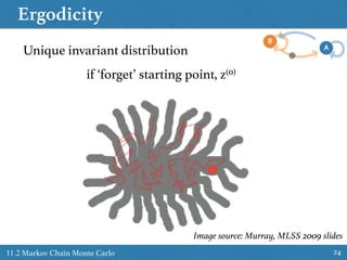
distribution (red curve)
q(z) =
c0
1 +
(z z0)2
d2
0
achieved by transforming z = d0 tan(⇡u) + z0
where u draw uniformly from [0, 1]
• We need to find z0, c0, d0 such that q(z) is greater (or equal) everywhere
to Gam(z|a,b) with smallest d0c0 (defines area)
z0 =
a 1
b
, d2
0 = 2a 1, c0 =
1
⇡d0](https://image.slidesharecdn.com/prmlreadingchapter11samplingmethodver2-160110083330/85/PRML-Reading-Chapter-11-Sampling-Method-10-320.jpg)
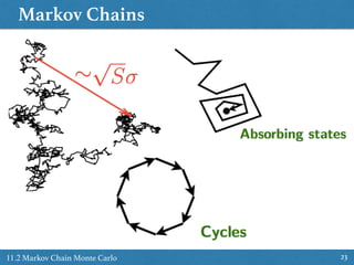
![Adaptive Rejection Sampling
1111.1 Basic Sampling Algorithms
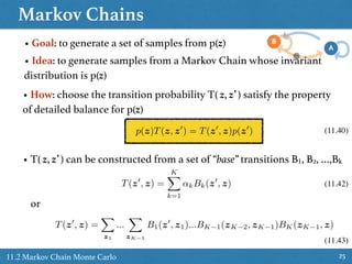
• The proposal distribution q(.) may be difficult to construct.
Fig 11.6: If a sample point is rejected, it is added to the set of the
grid points and used to refine the envelope distribution.
Construct
q(z) from
initial grid
points
Generate z4
from q(z)
Generate
u0 from
U[0, q(z4)]
Reject z4 if
Keep z4 if
• Rejection sampling methods
are inefficient if sampling in high
dimension (exponential decrease of
acceptance rate with dimensionality)
u0 ˜p(z4)
u0 > ˜p(z4)
but it is used to refine
the envelope
z4](https://image.slidesharecdn.com/prmlreadingchapter11samplingmethodver2-160110083330/85/PRML-Reading-Chapter-11-Sampling-Method-11-320.jpg)
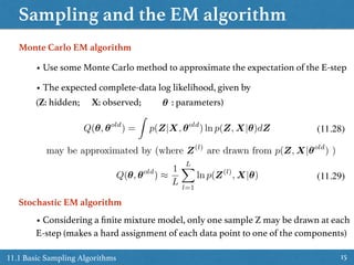
![Importance Sampling
1211.1 Basic Sampling Algorithms
IntegralBasic idea:
Transform the integral
into an expectation over a
simple, known
distribution
p(z) f(z)
z
q(z)
Conditions:
q(z) > 0 when f(z)p(z) ≠ 0
Easy to sample from q(z)
E[f] =
Z
f(z)p(z)dz
E[f] =
Z
f(z)p(z)
q(z)
q(z)
dz
E[f] =
Z
f(z)
p(z)
q(z)
q(z)dz
E[f] =
1
S
X
s
w(s)
f(z(s)
)
Proposal
Importance
weight
Monte Carlo
correct the bias
introduced by
sampling from a
wrong distribution
• All the generated samples are retained
Normalized
w(s)
/
p(z(s)
)
q(z(s))
z(s)
⇠ q(z)](https://image.slidesharecdn.com/prmlreadingchapter11samplingmethodver2-160110083330/85/PRML-Reading-Chapter-11-Sampling-Method-12-320.jpg)
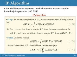


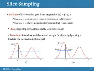
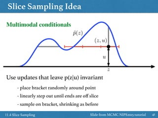
![Slice Sampling
3611.4 Slice Sampling
• Sample z and u uniformly from area under the distribution
✓ Fix z, sample u uniform from
✓ Fix u, sample z uniform from the slice through the distribution
• How to sample z from the slice
slice
[0, ˜p(z)]
{z : ˜p(z) > u}
✓ Start with the region of width w containing z(τ)
✓ If end point in slice, then extend region by w in that direction
✓ Sample z’ uniform from region
✓ If z’ in slice, then accept as z(τ+1)
✓ If not: make z’ new end point of the region, and resample z’
Multivariate distribution: slice
sampling within Gibbs sampler
See next slides for more details](https://image.slidesharecdn.com/prmlreadingchapter11samplingmethodver2-160110083330/85/PRML-Reading-Chapter-11-Sampling-Method-36-320.jpg)
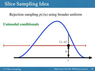
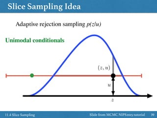
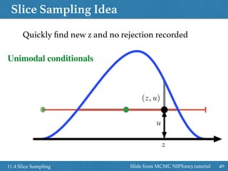
![Slice Sampling Idea
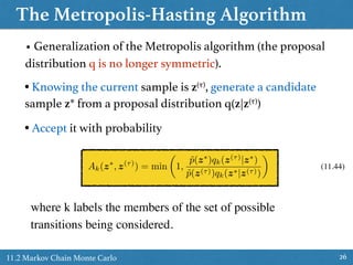
3711.4 Slice Sampling
˜p(z)
(z, u)
z
Sample uniformly under curve ˜p(z) / p(z)
p(u|z) = Uniform[0, ˜p(z)]
p(z|u) /
(
1 if ˜p(z) u
0 if otherwise
= Uniform on the slice
u
Slide from MCMC NIPS2015 tutorial](https://image.slidesharecdn.com/prmlreadingchapter11samplingmethodver2-160110083330/85/PRML-Reading-Chapter-11-Sampling-Method-37-320.jpg)


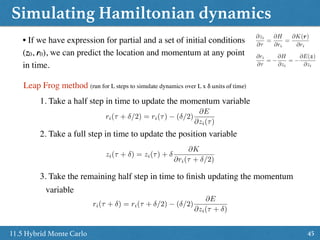

![Hybrid Monte Carlo
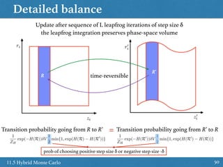
4811.5 Hybrid Monte Carlo
• Combination of Metropolis algorithm and Hamiltonian Dynamics
Algorithm to draw M samples from a target distribution
1. Set τ = 0
2. Generate an initial position state z(0) ~ π(0)
3. Repeat until τ = M
Set τ = τ + 1
- Sample a new initial momentum variable from the momentum canonical distribution r0 ~ p(r)
- Set z0 = z(τ - 1)
- Run Leap Frog algorithm starting at [z0, r0] for L step and step size δ to obtain proposed
states z* and r*
- Calculate the Metropolis acceptance probability
↵ = min(1, exp{H(z0, r0) H(z⇤
, r⇤
)})
- Draw a random number u uniformly from [0, 1]
If u ≤ α accept the position and set the next state z(τ) = z* else set z(τ)= z(τ-1)](https://image.slidesharecdn.com/prmlreadingchapter11samplingmethodver2-160110083330/85/PRML-Reading-Chapter-11-Sampling-Method-48-320.jpg)
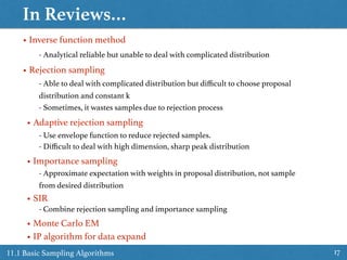
![Hybrid Monte Carlo simulation
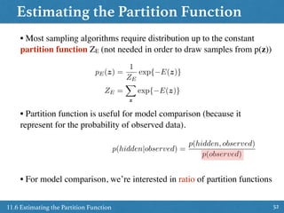
4911.5 Hybrid Monte Carlo
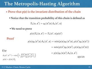
Hamiltonian Monte Carlo for sampling
a Bivariate Normal distribution
E(z) = log(e
zT ⌃ 1z
2 ) const
p(z) = N(µ, ⌃) with µ = [0, 0]
The MH algorithm converges much slower
than HMC, and consecutive samples have
much higher autocorrelation than samples
drawn using HMC
Img Source. https://theclevermachine.wordpress.com/2012/11/18/
mcmc-hamiltonian-monte-carlo-a-k-a-hybrid-monte-carlo/](https://image.slidesharecdn.com/prmlreadingchapter11samplingmethodver2-160110083330/85/PRML-Reading-Chapter-11-Sampling-Method-49-320.jpg)

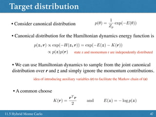
![Using importance sampling
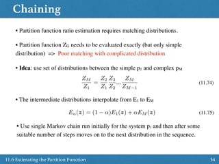
5311.6 Estimating the Partition Function
• Use importance sampling from proposal pG with energy G(z)
ZE
ZG
=
P
z exp( E(z))
P
z exp( G(z))
=
P
z exp( E(z) + G(z)) exp( G(z))
P
z exp( G(z))
= EpG
[exp( E(z) + G(z))] '
1
L
exp( E(z(l)
) + G(z(l)
)) (11.72)
sampled from pG
• Problem: pG need match pE
• Idea: we can use samples z(l) from pE from a Markov chain
• If ZG is easy to compute we can estimate ZE
pG(z) =
1
L
LX
l=1
T(z(l)
, z) (11.73)
where T gives the transition probabilities of the chain
• We now define G(z) = -log pG(z) and use in (11.72)](https://image.slidesharecdn.com/prmlreadingchapter11samplingmethodver2-160110083330/85/PRML-Reading-Chapter-11-Sampling-Method-53-320.jpg)


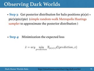
![Observing Dark Worlds
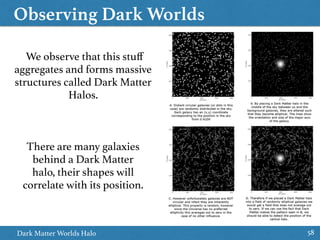
60Dark Matter Worlds Halo
https://www.kaggle.com/c/DarkWorlds• It is really one of statistics: given the noisy data (the elliptical galaxies)
recover the model and parameters (position and mass of the dark
matter) that generated them
• Step 1: construct a prior distribution p(x) for halo positions (e.g. uniform)
• Step 2: construct a probabilistic model for the data (observed ellipticities of
the galaxies) p(e|x) p(ei|x) = N(
X
j=allhalos
di,jmjf(ri,j), 2
)
http://timsalimans.com/observing-dark-worlds/
✦ dij = tangential direction, i.e. the direction in which halo j bends the light of galaxy i
✦ mj is the mass of halo j
✦ f(rij) is a decreasing function in the euclidean distance rij between galaxy i and halo j.
✦For the large halos assign m as a log-uniform distribution in [40,180], and f(rij) = 1/max(rij, 240)
✦For the small halos, fixed the mass at 20 and f(rij) = 1/max(rij, 70)](https://image.slidesharecdn.com/prmlreadingchapter11samplingmethodver2-160110083330/85/PRML-Reading-Chapter-11-Sampling-Method-60-320.jpg)

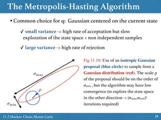
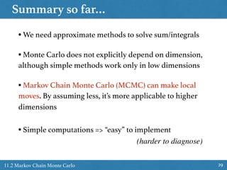
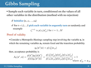
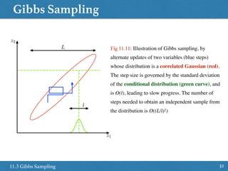
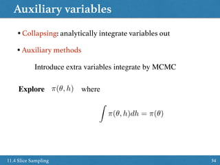
The document summarizes sampling methods from Chapter 11 of Bishop's PRML book. It introduces basic sampling algorithms like rejection sampling, importance sampling, and SIR. It then discusses Markov chain Monte Carlo (MCMC) methods which allow sampling from complex distributions using a Markov chain. Specific MCMC methods covered include the Metropolis algorithm, Gibbs sampling, and estimating the partition function using the IP algorithm.