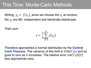
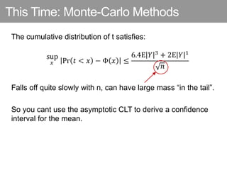
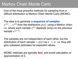
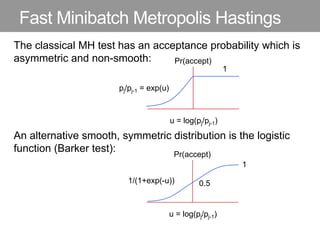
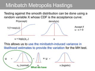
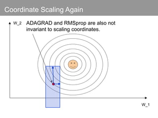
CS294-129: Designing, Visualizing and
Understanding Deep Neural Networks
John Canny
Fall 2016
Lecture 20: Monte-Carlo Methods
Last Time: Variational Auto-Encoders
Dependency:  - parametrized decoder:
 - parametrized encoder:
Both deep networks,
learned concurrently
Maximize the lower bound on log p(z|x)
jointly wrt  and :
Recall: Applications of Probabilistic Models
• Sampling
(synthesis)
• Autoencoding
(smile vectors):
Real Images Synthetic Images
Recall: Applications of Probabilistic Models
• Missing value imputation
• Density Estimation
• Denoising
This Time: Monte-Carlo Methods
Las Vegas: Fixed outcomes, random time
Monte-Carlo: Random outcomes
Outline: Monte-Carlo Methods
• Importance Sampling
• Markov Chain Monte-Carlo and Metropolis-Hastings
• Hamiltonian Monte-Carlo
• Langevin Dynamics
This Time: Monte-Carlo Methods
Sampling: Want to compute properties of a “difficult”
distribution as cheaply as possible:
• Take samples from a dataset
• Sample points in a model parameter space
• Sample latent (hidden) variables
The distribution is “difficult”:
• Sum or product of many components
• Not closed form
• The distribution may itself be parametric, and has to be
trained to approach reality.
This Time: Monte-Carlo Methods
Approximate Integrals:
Expected value of a function: E 𝑓 𝑥 = 𝑝 𝑥 𝑓 𝑥 𝑑𝑥
Or for discrete x, E 𝑓 𝑥 = 𝑖=1
𝑁
𝑝 𝑥𝑖 𝑓 𝑥𝑖
In both cases, we can approximate the expected value with a
sample of n values 𝑥1, … , 𝑥𝑛 from the distribution p(), giving:
𝑠 =
1
𝑛
𝑗=1
𝑛
𝑓 𝑥𝑗
This Time: Monte-Carlo Methods
Writing 𝑦𝑗 = 𝑓 𝑥𝑗 , since we choose the 𝑥𝑗 at random,
the 𝑦𝑗 are IID: independent and identically-distributed.
Their sum:
𝑠 =
1
𝑛
𝑗=1
𝑛
𝑓 𝑥𝑗
Therefore approaches a normal distribution by the Central
Limit Theorem. The variance of this limit is VAR 𝑌 /𝑛 and so
goes to zero as n increases. The relative error std 𝑌 /E 𝑌
also approaches zero.
This Time: Monte-Carlo Methods
Non Hand-Waving Central Limit Theorem:
Sample mean:
𝜇 =
1
𝑛
𝑖=1
𝑛
𝑦𝑖
Sample standard deviation:
𝑠 =
1
𝑛
𝑖=1
𝑛
𝑦𝑖 − 𝜇 2
Then the t-statistic t = 𝜇/s approaches a standard normal
distribution in the following sense:
This Time: Monte-Carlo Methods
The cumulative distribution of t satisfies:
𝑥
sup
Pr 𝑡 < 𝑥 − Φ 𝑥 ≤
6.4E 𝑌 3 + 2E 𝑌 1
𝑛
Where Φ 𝑥 is the cumulative distribution of the standard
Normal distribution (mean 0, variance 1).
E 𝑌 1 and E 𝑌 3 are the first and third absolute moments of
𝑌, i.e. expected first and third powers of 𝑌 − E 𝑌 .
This Time: Monte-Carlo Methods
The cumulative distribution of t satisfies:
𝑥
sup
Pr 𝑡 < 𝑥 − Φ 𝑥 ≤
6.4E 𝑌 3 + 2E 𝑌 1
𝑛
Falls off quite slowly with n, can have large mass “in the tail”.
So you cant use the asymptotic CLT to derive a confidence
interval for the mean.
Importance Sampling
Sampling from the true probability distribution p(x) can be
inefficient. The value we want is:
𝑠 =
1
𝑛
𝑗=1, 𝑥𝑗~𝑝(𝑥)
𝑛
𝑓 𝑥𝑗
Which has the same mean as:
𝑠𝑞 =
1
𝑛
𝑗=1, 𝑥𝑗~𝑞(𝑥)
𝑛
𝑝 𝑥𝑗 𝑓 𝑥𝑗
𝑞 𝑥𝑗
This is always an unbiased estimator, i.e. 𝐸 𝑠𝑞 = 𝐸 𝑠 = 𝜇,
but the variance depends strongly on the choice of sampling
distribution 𝑞 .
Importance Sampling
The variance is:
VAR 𝑌 =
1
𝑛
𝑗=1, 𝑥𝑗~𝑞(𝑥)
𝑛
𝑝 𝑥𝑗
𝑞 𝑥𝑗
2
𝑓 𝑥𝑗 − 𝜇
2
The optimal (minimum variance) 𝑞 is:
𝑞∗ 𝑥 =
𝑝 𝑥
𝑍
𝑓 𝑥 − 𝜇
where Z normalizes the 𝑞∗ 𝑥𝑖 to sum to 1 across possible
values of 𝑥𝑖.
i.e. choosing more extremal values of 𝑓 𝑥 improves
accuracy in estimating E 𝑓 𝑥
Importance Sampling
The weakness of this method is that we need to compute Z.
That can be expensive or impossible.
An alternative is to estimate Z, which we can do with:
𝑠𝐵𝐼𝑆 =
𝑗=1
𝑛 𝑝 𝑥𝑗
𝑞 𝑥𝑗
𝑓 𝑥𝑗
𝑗=1
𝑛 𝑝 𝑥𝑗
𝑞 𝑥𝑗
with 𝑥𝑗~𝑞 𝑥 . This estimator is biased for finite n, but
asymptotically unbiased as 𝑛 → ∞.
Markov Chain Monte Carlo
One of the most powerful methods for sampling from a
difficult distribution is Markov Chain Monte Carlo (MCMC).
The idea is to generate a sequence of samples
𝑥(1), … , 𝑥(𝑛) from the distribution 𝑝 𝑥 using a Markov chain.
i.e. where each sample 𝑥(𝑗) depends (only) on the previous
sample 𝑥(𝑗−1).
The samples are not independent of each other, but the
distribution of each sample → 𝑝 𝑥 as 𝑛 → ∞. i.e. they still
give unbiased estimates for expected values.
MCMC methods are typically fast, and avoid calculation or
approximation of Z.
Energy Representation
We can take negative logs as we do for likelihoods in
machine learning, yielding an Energy Based Model:
𝑝 𝑥 = exp −𝐸 𝑥
Note that if the energy is finite, 𝑝 𝑥 > 0.
A probability distribution in this form is called a
Boltzmann distribution.
Gibbs Sampling
Gibbs sampling is an efficient approach to generating
samples from the true distribution 𝑝 𝑥 using only the
unnormalized distribution 𝑝 𝑥 .
Taking each 𝑥𝑖 in turn, sample 𝑥𝑖 from 𝑝 𝑥𝑖|𝑥−𝑖 where 𝑥−𝑖 =
𝑥1, … , 𝑥𝑖−1, 𝑥𝑖+1, … , 𝑥𝑛
We need 𝑝 𝑥𝑖|𝑥−𝑖 to be normalized, but e.g. if 𝑥𝑖 has a small
discrete range, we can compute the unnormalized
probabilities for each value and normalize (c.f. softmax).
This is often easy because the energy is local, i.e. derived
from edge potentials in a graphical model.
Gibbs Sampling
Recall that energy for graphical models depends on local
potentials:
A
Nodes
Potential Functions
𝜑𝐴𝐵𝐷 B
E
D C
𝜑𝐷𝐸 𝜑𝐶𝐸
Can efficiently sample
D given A, B, E
Metropolis Hastings
Gibbs sampling assumes that we can not only evaluate
𝑝 𝑥𝑖|𝑥−𝑖 , but we can efficiently sample from 𝑝 . |𝑥−𝑖 .
This is only possible when the local probability distribution is
closed-form 𝑝 . |𝑥−𝑖 . Generally it isn’t.
When we don’t have a closed form local distribution, we can
still use a kind of rejection sampling to form a Markov chain.
For this we use a proposal distribution 𝑞 to choose the next
𝑥(𝑗)
~ 𝑞 . |𝑥(𝑗−1)
, and then accept-reject using the true
distribution p
Metropolis Hastings
The Metropolis-Hastings acceptance test accepts a proposed
𝑥(𝑗)
with probability p, where:
𝑝 𝑥(𝑗−1)
, 𝑥(𝑗)
= min 1,
𝑝 𝑥(𝑗) 𝑞 𝑥(𝑗−1)|𝑥(𝑗)
𝑝 𝑥(𝑗−1) 𝑞 𝑥(𝑗)|𝑥(𝑗−1)
This follows by considering transitions between the two states
𝑥(𝑗) and 𝑥(𝑗−1) :
We want detailed balance:
𝑝 𝑥(𝑗)|𝑥(𝑗−1)
𝑝 𝑥(𝑗−1)|𝑥(𝑗) =
𝑝 𝑥(𝑗)
𝑝 𝑥(𝑗−1)
p(x(j-1))
x(j-1)
p(x(j))
x(j)
p(x(j-1)|x(j) )
p(x(j)|x(j-1) )
Metropolis Hastings
Detailed balance
𝑝 𝑥(𝑗)|𝑥(𝑗−1)
𝑝 𝑥(𝑗−1)|𝑥(𝑗) =
𝑞 𝑥(𝑗)|𝑥(𝑗−1) 𝑝 𝑥(𝑗−1),𝑥(𝑗)
𝑞 𝑥(𝑗−1)|𝑥(𝑗) 𝑝 𝑥(𝑗),𝑥(𝑗−1)
𝑝 𝑥(𝑗−1),𝑥(𝑗)
𝑝 𝑥(𝑗),𝑥(𝑗−1) =
𝑝 𝑥(𝑗) 𝑞 𝑥(𝑗−1)|𝑥(𝑗)
𝑝 𝑥(𝑗−1) 𝑞 𝑥(𝑗)|𝑥(𝑗−1) substitute into the RHS, q’s
cancel, and we find:
𝑝 𝑥(𝑗)|𝑥(𝑗−1)
𝑝 𝑥(𝑗−1)|𝑥(𝑗)
=
𝑝 𝑥(𝑗)
𝑝 𝑥(𝑗−1)
p(x(j-1))
x(j-1)
p(x(j))
x(j)
p(x(j-1)|x(j) )
p(x(j)|x(j-1) )
Transition prob. proposal acceptance
acceptance
Metropolis Hastings
Metropolis-Hastings is very powerful and widely-used.
It reduces the problem of sampling from a difficult distribution
𝑝 𝑥 to making proposals: 𝑞 𝑥(𝑗)|𝑥(𝑗−1) and evaluating
ratios of 𝑝 𝑥(𝑗) /𝑝 𝑥(𝑗−1) .
The proposals can be trivial, e.g. random walk (choose 𝑥(𝑗)
from a normal distribution centered at 𝑥(𝑗−1)
), or sophisticated.
Only efficiency, not correctness is affected by the proposal.
Because only ratios 𝑝 𝑥(𝑗) /𝑝 𝑥(𝑗−1) are needed, we don’t
have to deal with normalizing sums Z.
Metropolis Hastings
M-H can be used for many applications, but has a serious
limitation when 𝑝 𝑥 depends on many observations, e.g.
when 𝑥 = 𝜃 are the parameters of a model.
Namely model parameters depend on all data points, and so
does the ratio:
𝑝 𝜃(𝑗)
/𝑝 𝜃(𝑗−1)
This forces batch updates (one per pass over the dataset)
which makes this kind of sampling very slow.
Until recently there was no fast way to perform M-H tests on
minibatches of data, which would allow SGD-style updates.
Fast Minibatch Metropolis Hastings
The classical MH test has an acceptance probability which is
asymmetric and non-smooth:
where 𝑝𝑗 is shorthand for 𝑝 𝑥(𝑗) .
Chu et al “An Efficient Minibatch Acceptance Test for Metropolis-Hastings” 2016
u = log(pj/pj-1)
Pr(accept) = min(1, pj/pj-1)
pj/pj-1 = exp(u)
1
Fast Minibatch Metropolis Hastings
The classical MH test has an acceptance probability which is
asymmetric and non-smooth:
An alternative smooth, symmetric distribution is the logistic
function (Barker test):
u = log(pj/pj-1)
Pr(accept)
pj/pj-1 = exp(u)
u = log(pj/pj-1)
Pr(accept)
1/(1+exp(-u))
1
1
0.5
Fast Minibatch Metropolis Hastings
The Barker test also satisfies detailed balance:
𝐿(𝑢)
𝐿(−𝑢)
= exp 𝑢 = 𝑝𝑗/𝑝𝑗−1
u = log(pj/pj-1)
Pr(accept)
1/(1+exp(-u))
L(u)
L(-u)
𝐿(𝑢)
𝐿(−𝑢)
= exp(𝑢)
u
-u
Logistic function L(u)
pj-1
x(j-1)
pj
x(j)
L(-u)
L(u)
Minibatch Metropolis Hastings
Testing against the smooth distribution can be done using a
random variable x whose CDF is the acceptance curve:
u = log(pj/pj-1)
Pr(accept)
1/(1+exp(u))
x
density(x)
Accept if
x < u
Minibatch Metropolis Hastings
Testing against the smooth distribution can be done using a
random variable X whose CDF is the acceptance curve:
This allows us to use the minibatch-induced variance in
likelihood estimates to provide the variation for the MH test.
u - - = u -
u = log(pj/pj-1)
Pr(accept)
1/(1+exp(u))
x
density(x)
Accept if
x < u
i.e.
u - x > 0
nU (normal) x (logistic)
xc
Minibatch Metropolis Hastings
Testing against the smooth distribution can be done using a
random variable X whose CDF is the acceptance curve:
This allows us to use the minibatch-induced variance in
likelihood estimates to provide the variation for the MH test.
u - - = u -
u = log(pj/pj-1)
Pr(accept)
1/(1+exp(u))
x
density(x)
Accept if
u - x > 0
nU (normal) x (logistic)
xc
What we have
Minibatch Metropolis Hastings
Testing against the smooth distribution can be done using a
random variable X whose CDF is the acceptance curve:
This allows us to use the minibatch-induced variance in
likelihood estimates to provide the variation for the MH test.
u - - = u -
u = log(pj/pj-1)
Pr(accept)
1/(1+exp(u))
x
density(x)
Accept if
u + x > 0
nU (normal) x (logistic)
xc
What we want
What we have
Minibatch Metropolis Hastings
This allows us to use the minibatch-induced variance in
likelihood estimates to provide the variation for the MH test.
u - - = u -
nU (minibatch
noise)
x (logistic)
xc
The variable x is the sum of nu and xc.
Its distribution is the convolution
of these two.
We can compute the distribution of xc
by deconvolution.
Exact
value
across
dataset
Minibatch Metropolis Hastings
The test itself is simple:
• Propose x(j) using q(x(j)| x(j-1)) from a minibatch of data.
• Compute u = log(pj/pj-1) = log(p(x(j))/p(x(j-1))) from another
minibatch.
• Sample xc from the correction distribution.
• Accept if u - xc > 0.
Minibatch Metropolis Hastings
• This approach has the same complexity as standard
SGD, with a small constant overhead.
• Minibatch sizes are fixed, acceptance probability is
reasonably high (around 0.5 typically).
• The variance in the log likelihood needs to be small (< 1).
• But this corresponds to “efficient” proposal distributions.
Hamiltonian Monte-Carlo
• Typical MCMC proposal are random walks. They lead to
very slow exploration of parameter space.
• Adding gradient bias seems like a natural step, but this
destroys detailed balance.
Hamiltonian Monte-Carlo
• Typical MCMC proposal are random walks. They lead to
very slow exploration of parameter space.
• Adding gradient bias seems like a natural step, but this
destroys detailed balance.
• We can restore detailed balance by introducing “fictitious”
state in the form of momentum variables.
• Now the state space is x (called “position”) and p (called
momentum). We augment the energy function as well.
• We recover the distribution of x, p(x) by “forgetting” the
momentum coordinates.
Hamiltonian Dynamics
Let x be position and p be momentum, H is an energy
function. The system evolves following:
𝑑𝑥𝑖
𝑑𝑡
=
𝜕𝐻
𝜕𝑝𝑖
and
𝑑𝑝𝑖
𝑑𝑡
= −
𝜕𝐻
𝜕𝑥𝑖
And typically:
𝐻 𝑥, 𝑝 = 𝑉 𝑥 + 1/2
𝑖=1
𝑛
𝑝𝑖
2
𝑚𝑖
Potential energy
(log probability(x))
Kinetic energy
(fictitious)
Total energy
Hamiltonian Dynamics
Typically: let x be position and p be momentum:
𝐻 𝑥, 𝑝 = 𝑉 𝑥 + 1/2
𝑖=1
𝑛
𝑝𝑖
2
𝑚𝑖
So
𝑑𝑥𝑖
𝑑𝑡
=
𝑝𝑖
𝑚𝑖
and
𝑑𝑝𝑖
𝑑𝑡
= −
𝜕𝑉
𝜕𝑥𝑖
Discretizing in time:
𝑝(𝑗) = 𝑝(𝑗−1) − 𝛻𝑉 𝑥(𝑗−1)
𝑥(𝑗) = 𝑥(𝑗−1) + 𝑚−1𝑝(𝑗−1)
Like SGD with no momentum decay.
Hamiltonian Monte-Carlo
Each iteration of HMC proceeds in two steps:
1. Sample momentum p from a zero-mean normal
distribution.
2. Do L times:
• Propose a new state (x,p) using Hamiltonian dynamics.
• Accept using an M-H test on the energy difference H.
• Note that momentum is only preserved through the steps
in the inner loop over L.
• Necessary to occasionally “spill” momentum so the
particle doesn’t have too much energy after descending.
Hamiltonian Monte-Carlo Animation
See https://www.youtube.com/watch?v=Vv3f0QNWvWQ
Langevin Dynamics
HMC:
• Have to periodically “reset” momentum.
• Need M-H tests on every sub-iteration.
Can we simulate a probabilistic system more directly?
Langevin dynamics:
𝑀𝑥 = −𝛻𝑉 − 𝛾𝑥 + 2𝛾𝑇𝒩(0,1)
mass x
acceleration
energy
gradient
viscous
damping
Noise (at
Temperature T)
Chen et al. “Stochastic Gradient Hamiltonian Monte-Carlo” 2014
Langevin Dynamics
Langevin dynamics:
𝑀𝑥 = −𝛻𝑉 − 𝛾𝑥 + 2𝛾𝑇𝒩(0,1)
Divide by M:
𝑥 = −
1
𝑀
𝛻𝑉 −
𝛾
𝑀
𝑥 +
2𝛾𝑇
𝑀
𝒩(0,1)
Discretize:
𝑥(𝑗) = 𝑣(𝑗) − 𝑣(𝑗−1)
𝑥(𝑗) = 𝑣(𝑗−1)
𝑥(𝑗) = 𝑥(𝑗−1) + 𝑣(𝑗)
Gives
𝑣(𝑗)
=
𝑀−𝛾
𝑀
𝑣(𝑗−1)
−
1
𝑀
𝛻𝑉 +
2𝛾𝑇
𝑀
𝒩 0,1
𝑥(𝑗)
= 𝑥(𝑗−1)
+ 𝑣(𝑗)
Langevin Dynamics
These equations are just SGD with momentum:
𝑣(𝑗) =
𝑀−𝛾
𝑀
𝑣(𝑗−1) −
1
𝑀
𝛻𝑉 +
2𝛾𝑇
𝑀
𝒩 0,1
𝑥(𝑗) = 𝑥(𝑗−1) + 𝑣(𝑗)
Can be written:
𝑣(𝑗) = 𝛼𝑣(𝑗−1) − 𝑙 𝛻𝑉 + 𝜖𝒩 0,1
𝑥(𝑗) = 𝑥(𝑗−1) + 𝑣(𝑗)
Where
• 𝛼 < 1 is “momentum”,
• 𝑙 is learning rate
• 𝜖 is minibatch noise in the gradient 𝛻𝑉
Langevin Dynamics
These equations are just SGD with momentum:
𝑣(𝑗) =
𝑀−𝛾
𝑀
𝑣(𝑗−1) −
1
𝑀
𝛻𝑉 +
2𝛾𝑇
𝑀
𝒩 0,1
𝑥(𝑗) = 𝑥(𝑗−1) + 𝑣(𝑗)
Can be written:
𝑣(𝑗) = 𝛼 𝑣(𝑗−1) − 𝑙 𝛻𝑉 + 𝜖 𝒩 0,1
𝑥(𝑗) = 𝑥(𝑗−1) + 𝑣(𝑗)
Can solve for 𝑀, 𝛾, 𝑇 given 𝛼, 𝑙, 𝜖 , i.e., we can translate
the standard SGD parameters into physical ones for the
simulated system.
Langevin Dynamics
i.e. Langevin dynamics agrees, up to step quantization
error, with the standard equations of SGD with momentum.
Remarkably, Langevin dynamics has a robust solution for
the stationary distribution of x:
𝑝 𝑥 = exp −
𝑉 𝑥
𝑇
The model allows us to control T even with significant noise
in the SGD gradients.
Langevin Dynamics
Notes:
• We so far assumed noise 𝒩 was generate by minibatch
variance only. But we can add noise explicitly to better
control the dynamics.
• We only used simplest possible quantization. Better
quantization, i.e. leapfrog steps can be used. This is
similar to using Nesterov momentum steps.
• M-H tests are still needed for optimal size steps (analysis
missing from Chen et al. paper).
Langevin Dynamics
Quick summary:
• Almost same cost as standard SGD with momentum.
• Using fast minibatch M-H testing and optimal step sizes,
cost increases about 2x.
• One sample generated per SGD/MH step. (HMC
generates one sample per L MH tests).
• Full posterior sampling at SGD rates.
Applications of HMC and Langevin
• Better characterization of the stationary distribution.
Control of temperature for annealing, mixing.
• Better quantized updates: Leapfrog method.
• Better understanding of coordinate scaling (ADAGRAD,
RMSprop, Natural gradient).
• Alternatives to variational smoothing.
original W
True negative gradient direction
W_1
W_2
Coordinate Scaling Again
ADAGRAD, RMSprop normalize gradient
coordinates, so gradients lie in a cube.
W_1
W_2
Coordinate Scaling Again
But this leads to higher variance of the
likelihood in the high gradient direction.
W_1
W_2
Coordinate Scaling Again
ADAGRAD and RMSprop are also not
invariant to scaling coordinates.
W_1
W_2
Coordinate Scaling Again
ADAGRAD and RMSprop are also not
invariant to scaling coordinates.
W_1
W_2
Coordinate Scaling Again
ADAGRAD’s implicit “working cube”, defined in the
analysis as D
W_1
W_2
Coordinate Scaling Again
CLAIM: such a cube matches well with the working range
of typical DNN parameters.
W_1
W_2
Coordinate Scaling Again
Coordinate Scaling Revisited
• For a variety of reasons, the ADAGRAD/RMSprop is poor
from an MCMC perspective.
• The optimal diagonal scaling, by several arguments, is:
𝑔𝑖 =
𝑔𝑖
𝐸 𝑔𝑖
2
• i.e. no square root in denominator as per ADAGRAD and
RMSprop.
• This update is invariant to coordinate transformations, and
minimizes bias and variance.
Coordinate Scaling Revisited
• For a variety of reasons, the ADAGRAD/RMSprop is poor
from an MCMC perspective.
• The optimal diagonal scaling, by several arguments, is:
𝑔𝑖 =
𝑔𝑖
𝐸 𝑔𝑖
2
• i.e. no square root in denominator as per ADAGRAD and
RMSprop.
• In practice, it may be prone to “exploding” when 𝐸 𝑔𝑖
2
is
small. But when “working range” is taken into account,
𝐸 𝑔𝑖
2
should never be too small.
Model the working range with a regularizing norm on x as
part of V(x). Then 𝑔𝑖
2
will never be too small.
W_1
W_2
Optimal Coordinate Scaling Again
Optimal g scaling
Coordinate Scaling Revisited
Optimal coordinate scaling for HMC and Langevin:
Girolami et al. 2014 “Riemann Manifold Langevin and Hamiltonian
Monte Carlo”
Practical performance of gradient scaling methods:
Yann Ollivier, 2015 “Riemannian metrics for neural networks I:
Feedforward networks”
Takeaways
• Importance Sampling is used to
estimate means with fewer samples.
• Monte-Carlo sampling requires either:
• Closed form local distributions (Gibbs sampling)
• A proposal distribution and acceptance test (M-H).
• M-H tests keep samples in known distribution. Proposals
only affect speed.
• There are alternatives to the Metropolis-Hastings test
(Barker test) which works fast on minibatches of data.
Performance is similar to vanilla SGD.
Takeaways
• Hamiltonian Monte Carlo (HMC)
adds a momentum term to allow
non-reversible (gradient) proposals.
• Langevin dynamics adds a damping term to standard HMC.
Can take larger steps with fewer M-H tests.
• Applications of MCMC methods:
• Better training parameter setting.
• Controlled annealing and tempering.
• Efficient full posterior inference.

Monte Carlo Berkeley.pptx

  • 1.
    CS294-129: Designing, Visualizingand Understanding Deep Neural Networks John Canny Fall 2016 Lecture 20: Monte-Carlo Methods
  • 2.
    Last Time: VariationalAuto-Encoders Dependency:  - parametrized decoder:  - parametrized encoder: Both deep networks, learned concurrently Maximize the lower bound on log p(z|x) jointly wrt  and :
  • 3.
    Recall: Applications ofProbabilistic Models • Sampling (synthesis) • Autoencoding (smile vectors): Real Images Synthetic Images
  • 4.
    Recall: Applications ofProbabilistic Models • Missing value imputation • Density Estimation • Denoising
  • 5.
    This Time: Monte-CarloMethods Las Vegas: Fixed outcomes, random time Monte-Carlo: Random outcomes
  • 6.
    Outline: Monte-Carlo Methods •Importance Sampling • Markov Chain Monte-Carlo and Metropolis-Hastings • Hamiltonian Monte-Carlo • Langevin Dynamics
  • 7.
    This Time: Monte-CarloMethods Sampling: Want to compute properties of a “difficult” distribution as cheaply as possible: • Take samples from a dataset • Sample points in a model parameter space • Sample latent (hidden) variables The distribution is “difficult”: • Sum or product of many components • Not closed form • The distribution may itself be parametric, and has to be trained to approach reality.
  • 8.
    This Time: Monte-CarloMethods Approximate Integrals: Expected value of a function: E 𝑓 𝑥 = 𝑝 𝑥 𝑓 𝑥 𝑑𝑥 Or for discrete x, E 𝑓 𝑥 = 𝑖=1 𝑁 𝑝 𝑥𝑖 𝑓 𝑥𝑖 In both cases, we can approximate the expected value with a sample of n values 𝑥1, … , 𝑥𝑛 from the distribution p(), giving: 𝑠 = 1 𝑛 𝑗=1 𝑛 𝑓 𝑥𝑗
  • 9.
    This Time: Monte-CarloMethods Writing 𝑦𝑗 = 𝑓 𝑥𝑗 , since we choose the 𝑥𝑗 at random, the 𝑦𝑗 are IID: independent and identically-distributed. Their sum: 𝑠 = 1 𝑛 𝑗=1 𝑛 𝑓 𝑥𝑗 Therefore approaches a normal distribution by the Central Limit Theorem. The variance of this limit is VAR 𝑌 /𝑛 and so goes to zero as n increases. The relative error std 𝑌 /E 𝑌 also approaches zero.
  • 10.
    This Time: Monte-CarloMethods Non Hand-Waving Central Limit Theorem: Sample mean: 𝜇 = 1 𝑛 𝑖=1 𝑛 𝑦𝑖 Sample standard deviation: 𝑠 = 1 𝑛 𝑖=1 𝑛 𝑦𝑖 − 𝜇 2 Then the t-statistic t = 𝜇/s approaches a standard normal distribution in the following sense:
  • 11.
    This Time: Monte-CarloMethods The cumulative distribution of t satisfies: 𝑥 sup Pr 𝑡 < 𝑥 − Φ 𝑥 ≤ 6.4E 𝑌 3 + 2E 𝑌 1 𝑛 Where Φ 𝑥 is the cumulative distribution of the standard Normal distribution (mean 0, variance 1). E 𝑌 1 and E 𝑌 3 are the first and third absolute moments of 𝑌, i.e. expected first and third powers of 𝑌 − E 𝑌 .
  • 12.
    This Time: Monte-CarloMethods The cumulative distribution of t satisfies: 𝑥 sup Pr 𝑡 < 𝑥 − Φ 𝑥 ≤ 6.4E 𝑌 3 + 2E 𝑌 1 𝑛 Falls off quite slowly with n, can have large mass “in the tail”. So you cant use the asymptotic CLT to derive a confidence interval for the mean.
  • 13.
    Importance Sampling Sampling fromthe true probability distribution p(x) can be inefficient. The value we want is: 𝑠 = 1 𝑛 𝑗=1, 𝑥𝑗~𝑝(𝑥) 𝑛 𝑓 𝑥𝑗 Which has the same mean as: 𝑠𝑞 = 1 𝑛 𝑗=1, 𝑥𝑗~𝑞(𝑥) 𝑛 𝑝 𝑥𝑗 𝑓 𝑥𝑗 𝑞 𝑥𝑗 This is always an unbiased estimator, i.e. 𝐸 𝑠𝑞 = 𝐸 𝑠 = 𝜇, but the variance depends strongly on the choice of sampling distribution 𝑞 .
  • 14.
    Importance Sampling The varianceis: VAR 𝑌 = 1 𝑛 𝑗=1, 𝑥𝑗~𝑞(𝑥) 𝑛 𝑝 𝑥𝑗 𝑞 𝑥𝑗 2 𝑓 𝑥𝑗 − 𝜇 2 The optimal (minimum variance) 𝑞 is: 𝑞∗ 𝑥 = 𝑝 𝑥 𝑍 𝑓 𝑥 − 𝜇 where Z normalizes the 𝑞∗ 𝑥𝑖 to sum to 1 across possible values of 𝑥𝑖. i.e. choosing more extremal values of 𝑓 𝑥 improves accuracy in estimating E 𝑓 𝑥
  • 15.
    Importance Sampling The weaknessof this method is that we need to compute Z. That can be expensive or impossible. An alternative is to estimate Z, which we can do with: 𝑠𝐵𝐼𝑆 = 𝑗=1 𝑛 𝑝 𝑥𝑗 𝑞 𝑥𝑗 𝑓 𝑥𝑗 𝑗=1 𝑛 𝑝 𝑥𝑗 𝑞 𝑥𝑗 with 𝑥𝑗~𝑞 𝑥 . This estimator is biased for finite n, but asymptotically unbiased as 𝑛 → ∞.
  • 16.
    Markov Chain MonteCarlo One of the most powerful methods for sampling from a difficult distribution is Markov Chain Monte Carlo (MCMC). The idea is to generate a sequence of samples 𝑥(1), … , 𝑥(𝑛) from the distribution 𝑝 𝑥 using a Markov chain. i.e. where each sample 𝑥(𝑗) depends (only) on the previous sample 𝑥(𝑗−1). The samples are not independent of each other, but the distribution of each sample → 𝑝 𝑥 as 𝑛 → ∞. i.e. they still give unbiased estimates for expected values. MCMC methods are typically fast, and avoid calculation or approximation of Z.
  • 17.
    Energy Representation We cantake negative logs as we do for likelihoods in machine learning, yielding an Energy Based Model: 𝑝 𝑥 = exp −𝐸 𝑥 Note that if the energy is finite, 𝑝 𝑥 > 0. A probability distribution in this form is called a Boltzmann distribution.
  • 18.
    Gibbs Sampling Gibbs samplingis an efficient approach to generating samples from the true distribution 𝑝 𝑥 using only the unnormalized distribution 𝑝 𝑥 . Taking each 𝑥𝑖 in turn, sample 𝑥𝑖 from 𝑝 𝑥𝑖|𝑥−𝑖 where 𝑥−𝑖 = 𝑥1, … , 𝑥𝑖−1, 𝑥𝑖+1, … , 𝑥𝑛 We need 𝑝 𝑥𝑖|𝑥−𝑖 to be normalized, but e.g. if 𝑥𝑖 has a small discrete range, we can compute the unnormalized probabilities for each value and normalize (c.f. softmax). This is often easy because the energy is local, i.e. derived from edge potentials in a graphical model.
  • 19.
    Gibbs Sampling Recall thatenergy for graphical models depends on local potentials: A Nodes Potential Functions 𝜑𝐴𝐵𝐷 B E D C 𝜑𝐷𝐸 𝜑𝐶𝐸 Can efficiently sample D given A, B, E
  • 20.
    Metropolis Hastings Gibbs samplingassumes that we can not only evaluate 𝑝 𝑥𝑖|𝑥−𝑖 , but we can efficiently sample from 𝑝 . |𝑥−𝑖 . This is only possible when the local probability distribution is closed-form 𝑝 . |𝑥−𝑖 . Generally it isn’t. When we don’t have a closed form local distribution, we can still use a kind of rejection sampling to form a Markov chain. For this we use a proposal distribution 𝑞 to choose the next 𝑥(𝑗) ~ 𝑞 . |𝑥(𝑗−1) , and then accept-reject using the true distribution p
  • 21.
    Metropolis Hastings The Metropolis-Hastingsacceptance test accepts a proposed 𝑥(𝑗) with probability p, where: 𝑝 𝑥(𝑗−1) , 𝑥(𝑗) = min 1, 𝑝 𝑥(𝑗) 𝑞 𝑥(𝑗−1)|𝑥(𝑗) 𝑝 𝑥(𝑗−1) 𝑞 𝑥(𝑗)|𝑥(𝑗−1) This follows by considering transitions between the two states 𝑥(𝑗) and 𝑥(𝑗−1) : We want detailed balance: 𝑝 𝑥(𝑗)|𝑥(𝑗−1) 𝑝 𝑥(𝑗−1)|𝑥(𝑗) = 𝑝 𝑥(𝑗) 𝑝 𝑥(𝑗−1) p(x(j-1)) x(j-1) p(x(j)) x(j) p(x(j-1)|x(j) ) p(x(j)|x(j-1) )
  • 22.
    Metropolis Hastings Detailed balance 𝑝𝑥(𝑗)|𝑥(𝑗−1) 𝑝 𝑥(𝑗−1)|𝑥(𝑗) = 𝑞 𝑥(𝑗)|𝑥(𝑗−1) 𝑝 𝑥(𝑗−1),𝑥(𝑗) 𝑞 𝑥(𝑗−1)|𝑥(𝑗) 𝑝 𝑥(𝑗),𝑥(𝑗−1) 𝑝 𝑥(𝑗−1),𝑥(𝑗) 𝑝 𝑥(𝑗),𝑥(𝑗−1) = 𝑝 𝑥(𝑗) 𝑞 𝑥(𝑗−1)|𝑥(𝑗) 𝑝 𝑥(𝑗−1) 𝑞 𝑥(𝑗)|𝑥(𝑗−1) substitute into the RHS, q’s cancel, and we find: 𝑝 𝑥(𝑗)|𝑥(𝑗−1) 𝑝 𝑥(𝑗−1)|𝑥(𝑗) = 𝑝 𝑥(𝑗) 𝑝 𝑥(𝑗−1) p(x(j-1)) x(j-1) p(x(j)) x(j) p(x(j-1)|x(j) ) p(x(j)|x(j-1) ) Transition prob. proposal acceptance acceptance
  • 23.
    Metropolis Hastings Metropolis-Hastings isvery powerful and widely-used. It reduces the problem of sampling from a difficult distribution 𝑝 𝑥 to making proposals: 𝑞 𝑥(𝑗)|𝑥(𝑗−1) and evaluating ratios of 𝑝 𝑥(𝑗) /𝑝 𝑥(𝑗−1) . The proposals can be trivial, e.g. random walk (choose 𝑥(𝑗) from a normal distribution centered at 𝑥(𝑗−1) ), or sophisticated. Only efficiency, not correctness is affected by the proposal. Because only ratios 𝑝 𝑥(𝑗) /𝑝 𝑥(𝑗−1) are needed, we don’t have to deal with normalizing sums Z.
  • 24.
    Metropolis Hastings M-H canbe used for many applications, but has a serious limitation when 𝑝 𝑥 depends on many observations, e.g. when 𝑥 = 𝜃 are the parameters of a model. Namely model parameters depend on all data points, and so does the ratio: 𝑝 𝜃(𝑗) /𝑝 𝜃(𝑗−1) This forces batch updates (one per pass over the dataset) which makes this kind of sampling very slow. Until recently there was no fast way to perform M-H tests on minibatches of data, which would allow SGD-style updates.
  • 25.
    Fast Minibatch MetropolisHastings The classical MH test has an acceptance probability which is asymmetric and non-smooth: where 𝑝𝑗 is shorthand for 𝑝 𝑥(𝑗) . Chu et al “An Efficient Minibatch Acceptance Test for Metropolis-Hastings” 2016 u = log(pj/pj-1) Pr(accept) = min(1, pj/pj-1) pj/pj-1 = exp(u) 1
  • 26.
    Fast Minibatch MetropolisHastings The classical MH test has an acceptance probability which is asymmetric and non-smooth: An alternative smooth, symmetric distribution is the logistic function (Barker test): u = log(pj/pj-1) Pr(accept) pj/pj-1 = exp(u) u = log(pj/pj-1) Pr(accept) 1/(1+exp(-u)) 1 1 0.5
  • 27.
    Fast Minibatch MetropolisHastings The Barker test also satisfies detailed balance: 𝐿(𝑢) 𝐿(−𝑢) = exp 𝑢 = 𝑝𝑗/𝑝𝑗−1 u = log(pj/pj-1) Pr(accept) 1/(1+exp(-u)) L(u) L(-u) 𝐿(𝑢) 𝐿(−𝑢) = exp(𝑢) u -u Logistic function L(u) pj-1 x(j-1) pj x(j) L(-u) L(u)
  • 28.
    Minibatch Metropolis Hastings Testingagainst the smooth distribution can be done using a random variable x whose CDF is the acceptance curve: u = log(pj/pj-1) Pr(accept) 1/(1+exp(u)) x density(x) Accept if x < u
  • 29.
    Minibatch Metropolis Hastings Testingagainst the smooth distribution can be done using a random variable X whose CDF is the acceptance curve: This allows us to use the minibatch-induced variance in likelihood estimates to provide the variation for the MH test. u - - = u - u = log(pj/pj-1) Pr(accept) 1/(1+exp(u)) x density(x) Accept if x < u i.e. u - x > 0 nU (normal) x (logistic) xc
  • 30.
    Minibatch Metropolis Hastings Testingagainst the smooth distribution can be done using a random variable X whose CDF is the acceptance curve: This allows us to use the minibatch-induced variance in likelihood estimates to provide the variation for the MH test. u - - = u - u = log(pj/pj-1) Pr(accept) 1/(1+exp(u)) x density(x) Accept if u - x > 0 nU (normal) x (logistic) xc What we have
  • 31.
    Minibatch Metropolis Hastings Testingagainst the smooth distribution can be done using a random variable X whose CDF is the acceptance curve: This allows us to use the minibatch-induced variance in likelihood estimates to provide the variation for the MH test. u - - = u - u = log(pj/pj-1) Pr(accept) 1/(1+exp(u)) x density(x) Accept if u + x > 0 nU (normal) x (logistic) xc What we want What we have
  • 32.
    Minibatch Metropolis Hastings Thisallows us to use the minibatch-induced variance in likelihood estimates to provide the variation for the MH test. u - - = u - nU (minibatch noise) x (logistic) xc The variable x is the sum of nu and xc. Its distribution is the convolution of these two. We can compute the distribution of xc by deconvolution. Exact value across dataset
  • 33.
    Minibatch Metropolis Hastings Thetest itself is simple: • Propose x(j) using q(x(j)| x(j-1)) from a minibatch of data. • Compute u = log(pj/pj-1) = log(p(x(j))/p(x(j-1))) from another minibatch. • Sample xc from the correction distribution. • Accept if u - xc > 0.
  • 34.
    Minibatch Metropolis Hastings •This approach has the same complexity as standard SGD, with a small constant overhead. • Minibatch sizes are fixed, acceptance probability is reasonably high (around 0.5 typically). • The variance in the log likelihood needs to be small (< 1). • But this corresponds to “efficient” proposal distributions.
  • 35.
    Hamiltonian Monte-Carlo • TypicalMCMC proposal are random walks. They lead to very slow exploration of parameter space. • Adding gradient bias seems like a natural step, but this destroys detailed balance.
  • 36.
    Hamiltonian Monte-Carlo • TypicalMCMC proposal are random walks. They lead to very slow exploration of parameter space. • Adding gradient bias seems like a natural step, but this destroys detailed balance. • We can restore detailed balance by introducing “fictitious” state in the form of momentum variables. • Now the state space is x (called “position”) and p (called momentum). We augment the energy function as well. • We recover the distribution of x, p(x) by “forgetting” the momentum coordinates.
  • 37.
    Hamiltonian Dynamics Let xbe position and p be momentum, H is an energy function. The system evolves following: 𝑑𝑥𝑖 𝑑𝑡 = 𝜕𝐻 𝜕𝑝𝑖 and 𝑑𝑝𝑖 𝑑𝑡 = − 𝜕𝐻 𝜕𝑥𝑖 And typically: 𝐻 𝑥, 𝑝 = 𝑉 𝑥 + 1/2 𝑖=1 𝑛 𝑝𝑖 2 𝑚𝑖 Potential energy (log probability(x)) Kinetic energy (fictitious) Total energy
  • 38.
    Hamiltonian Dynamics Typically: letx be position and p be momentum: 𝐻 𝑥, 𝑝 = 𝑉 𝑥 + 1/2 𝑖=1 𝑛 𝑝𝑖 2 𝑚𝑖 So 𝑑𝑥𝑖 𝑑𝑡 = 𝑝𝑖 𝑚𝑖 and 𝑑𝑝𝑖 𝑑𝑡 = − 𝜕𝑉 𝜕𝑥𝑖 Discretizing in time: 𝑝(𝑗) = 𝑝(𝑗−1) − 𝛻𝑉 𝑥(𝑗−1) 𝑥(𝑗) = 𝑥(𝑗−1) + 𝑚−1𝑝(𝑗−1) Like SGD with no momentum decay.
  • 39.
    Hamiltonian Monte-Carlo Each iterationof HMC proceeds in two steps: 1. Sample momentum p from a zero-mean normal distribution. 2. Do L times: • Propose a new state (x,p) using Hamiltonian dynamics. • Accept using an M-H test on the energy difference H. • Note that momentum is only preserved through the steps in the inner loop over L. • Necessary to occasionally “spill” momentum so the particle doesn’t have too much energy after descending.
  • 40.
    Hamiltonian Monte-Carlo Animation Seehttps://www.youtube.com/watch?v=Vv3f0QNWvWQ
  • 41.
    Langevin Dynamics HMC: • Haveto periodically “reset” momentum. • Need M-H tests on every sub-iteration. Can we simulate a probabilistic system more directly? Langevin dynamics: 𝑀𝑥 = −𝛻𝑉 − 𝛾𝑥 + 2𝛾𝑇𝒩(0,1) mass x acceleration energy gradient viscous damping Noise (at Temperature T) Chen et al. “Stochastic Gradient Hamiltonian Monte-Carlo” 2014
  • 42.
    Langevin Dynamics Langevin dynamics: 𝑀𝑥= −𝛻𝑉 − 𝛾𝑥 + 2𝛾𝑇𝒩(0,1) Divide by M: 𝑥 = − 1 𝑀 𝛻𝑉 − 𝛾 𝑀 𝑥 + 2𝛾𝑇 𝑀 𝒩(0,1) Discretize: 𝑥(𝑗) = 𝑣(𝑗) − 𝑣(𝑗−1) 𝑥(𝑗) = 𝑣(𝑗−1) 𝑥(𝑗) = 𝑥(𝑗−1) + 𝑣(𝑗) Gives 𝑣(𝑗) = 𝑀−𝛾 𝑀 𝑣(𝑗−1) − 1 𝑀 𝛻𝑉 + 2𝛾𝑇 𝑀 𝒩 0,1 𝑥(𝑗) = 𝑥(𝑗−1) + 𝑣(𝑗)
  • 43.
    Langevin Dynamics These equationsare just SGD with momentum: 𝑣(𝑗) = 𝑀−𝛾 𝑀 𝑣(𝑗−1) − 1 𝑀 𝛻𝑉 + 2𝛾𝑇 𝑀 𝒩 0,1 𝑥(𝑗) = 𝑥(𝑗−1) + 𝑣(𝑗) Can be written: 𝑣(𝑗) = 𝛼𝑣(𝑗−1) − 𝑙 𝛻𝑉 + 𝜖𝒩 0,1 𝑥(𝑗) = 𝑥(𝑗−1) + 𝑣(𝑗) Where • 𝛼 < 1 is “momentum”, • 𝑙 is learning rate • 𝜖 is minibatch noise in the gradient 𝛻𝑉
  • 44.
    Langevin Dynamics These equationsare just SGD with momentum: 𝑣(𝑗) = 𝑀−𝛾 𝑀 𝑣(𝑗−1) − 1 𝑀 𝛻𝑉 + 2𝛾𝑇 𝑀 𝒩 0,1 𝑥(𝑗) = 𝑥(𝑗−1) + 𝑣(𝑗) Can be written: 𝑣(𝑗) = 𝛼 𝑣(𝑗−1) − 𝑙 𝛻𝑉 + 𝜖 𝒩 0,1 𝑥(𝑗) = 𝑥(𝑗−1) + 𝑣(𝑗) Can solve for 𝑀, 𝛾, 𝑇 given 𝛼, 𝑙, 𝜖 , i.e., we can translate the standard SGD parameters into physical ones for the simulated system.
  • 45.
    Langevin Dynamics i.e. Langevindynamics agrees, up to step quantization error, with the standard equations of SGD with momentum. Remarkably, Langevin dynamics has a robust solution for the stationary distribution of x: 𝑝 𝑥 = exp − 𝑉 𝑥 𝑇 The model allows us to control T even with significant noise in the SGD gradients.
  • 46.
    Langevin Dynamics Notes: • Weso far assumed noise 𝒩 was generate by minibatch variance only. But we can add noise explicitly to better control the dynamics. • We only used simplest possible quantization. Better quantization, i.e. leapfrog steps can be used. This is similar to using Nesterov momentum steps. • M-H tests are still needed for optimal size steps (analysis missing from Chen et al. paper).
  • 47.
    Langevin Dynamics Quick summary: •Almost same cost as standard SGD with momentum. • Using fast minibatch M-H testing and optimal step sizes, cost increases about 2x. • One sample generated per SGD/MH step. (HMC generates one sample per L MH tests). • Full posterior sampling at SGD rates.
  • 48.
    Applications of HMCand Langevin • Better characterization of the stationary distribution. Control of temperature for annealing, mixing. • Better quantized updates: Leapfrog method. • Better understanding of coordinate scaling (ADAGRAD, RMSprop, Natural gradient). • Alternatives to variational smoothing.
  • 49.
    original W True negativegradient direction W_1 W_2 Coordinate Scaling Again
  • 50.
    ADAGRAD, RMSprop normalizegradient coordinates, so gradients lie in a cube. W_1 W_2 Coordinate Scaling Again
  • 51.
    But this leadsto higher variance of the likelihood in the high gradient direction. W_1 W_2 Coordinate Scaling Again
  • 52.
    ADAGRAD and RMSpropare also not invariant to scaling coordinates. W_1 W_2 Coordinate Scaling Again
  • 53.
    ADAGRAD and RMSpropare also not invariant to scaling coordinates. W_1 W_2 Coordinate Scaling Again
  • 54.
    ADAGRAD’s implicit “workingcube”, defined in the analysis as D W_1 W_2 Coordinate Scaling Again
  • 55.
    CLAIM: such acube matches well with the working range of typical DNN parameters. W_1 W_2 Coordinate Scaling Again
  • 56.
    Coordinate Scaling Revisited •For a variety of reasons, the ADAGRAD/RMSprop is poor from an MCMC perspective. • The optimal diagonal scaling, by several arguments, is: 𝑔𝑖 = 𝑔𝑖 𝐸 𝑔𝑖 2 • i.e. no square root in denominator as per ADAGRAD and RMSprop. • This update is invariant to coordinate transformations, and minimizes bias and variance.
  • 57.
    Coordinate Scaling Revisited •For a variety of reasons, the ADAGRAD/RMSprop is poor from an MCMC perspective. • The optimal diagonal scaling, by several arguments, is: 𝑔𝑖 = 𝑔𝑖 𝐸 𝑔𝑖 2 • i.e. no square root in denominator as per ADAGRAD and RMSprop. • In practice, it may be prone to “exploding” when 𝐸 𝑔𝑖 2 is small. But when “working range” is taken into account, 𝐸 𝑔𝑖 2 should never be too small.
  • 58.
    Model the workingrange with a regularizing norm on x as part of V(x). Then 𝑔𝑖 2 will never be too small. W_1 W_2 Optimal Coordinate Scaling Again Optimal g scaling
  • 59.
    Coordinate Scaling Revisited Optimalcoordinate scaling for HMC and Langevin: Girolami et al. 2014 “Riemann Manifold Langevin and Hamiltonian Monte Carlo” Practical performance of gradient scaling methods: Yann Ollivier, 2015 “Riemannian metrics for neural networks I: Feedforward networks”
  • 60.
    Takeaways • Importance Samplingis used to estimate means with fewer samples. • Monte-Carlo sampling requires either: • Closed form local distributions (Gibbs sampling) • A proposal distribution and acceptance test (M-H). • M-H tests keep samples in known distribution. Proposals only affect speed. • There are alternatives to the Metropolis-Hastings test (Barker test) which works fast on minibatches of data. Performance is similar to vanilla SGD.
  • 61.
    Takeaways • Hamiltonian MonteCarlo (HMC) adds a momentum term to allow non-reversible (gradient) proposals. • Langevin dynamics adds a damping term to standard HMC. Can take larger steps with fewer M-H tests. • Applications of MCMC methods: • Better training parameter setting. • Controlled annealing and tempering. • Efficient full posterior inference.