Downloaded 17 times

![Chapter 10.3. Variational Linear Regression
22
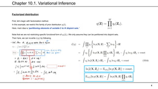
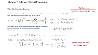
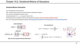
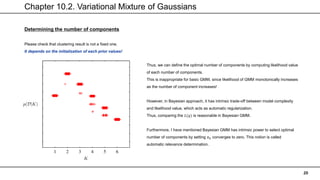
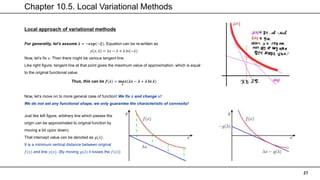
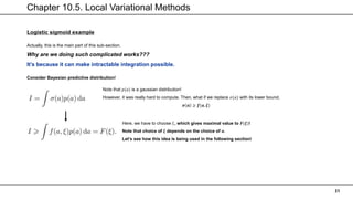
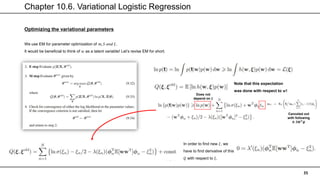
Fully Bayesian linear regression
Since it has a form of gamma distribution, we can approximate this variational distribution by gamma!
This way, we can find 𝑞(𝛼). Similarly,
we can get a distribution of 𝑤.
Note that the term of 𝑤 exist in a quadratic form, which indicates a
gaussian distribution!
Note that overall equation only differs at the 𝑬[𝜶] from chp 3.
This expression becomes relatively similar to that of EM, when we
set α0 = β0 = 0, which means we are not having any prior
knowledge about the parameter 𝜶](https://image.slidesharecdn.com/chapter10-210805144218/85/PRML-Chapter-10-22-320.jpg)
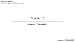
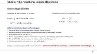
![Chapter 10.3. Variational Linear Regression
23
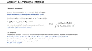
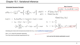
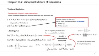
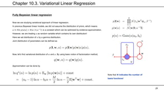
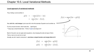
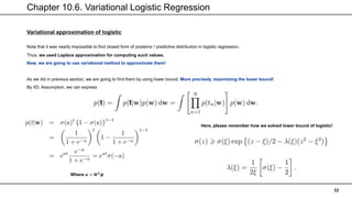
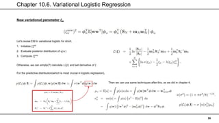
Predictive distribution & Lower bound of variational linear regression
Big idea is same. Just details are different.
But here, we are using 𝐸[𝛼] instead of simple 𝛼
Similarly, we can evaluate lower bound to compare different models.
Ground-Truth : 𝑋3
𝑥 − 𝑎𝑥𝑖𝑠 ∶ 𝑃𝑜𝑙𝑦𝑛𝑜𝑚𝑖𝑎𝑙 𝑜𝑓 𝑋
𝑦 − 𝑎𝑥𝑖𝑠 ∶ 𝐿(𝑞)
We can see it is being maximized in 𝑴 = 𝟑](https://image.slidesharecdn.com/chapter10-210805144218/85/PRML-Chapter-10-23-320.jpg)
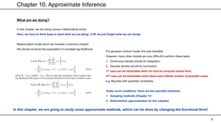
![Chapter 10.4. Exponential Family Distributions
25
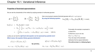
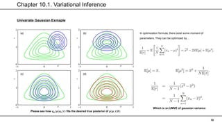
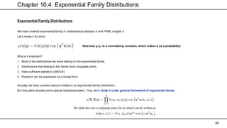
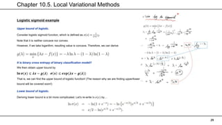
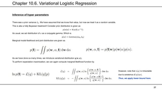
Variational distribution
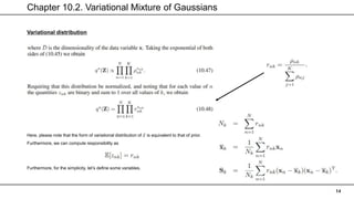
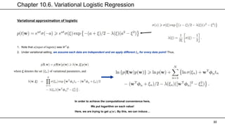
Now, we have to define variational distribution of 𝑧.
Here, 𝒒 𝒁, 𝜼 = 𝒒 𝒁 𝒒(𝜼). According to formula, we can re-write it by
Variational distribution can be
decomposed into each individual data
E – Step : Computing 𝐸𝜂[𝑢(𝑥𝑛, 𝑧𝑛)] / Filling unseen-latent variable.
M - Step : Updating each distributions.
Furthermore, we can write this
In variational message passing!](https://image.slidesharecdn.com/chapter10-210805144218/85/PRML-Chapter-10-25-320.jpg)

This chapter discusses approximate inference methods for probabilistic models where exact inference is intractable. It introduces variational inference as a deterministic approximation approach. Variational inference works by restricting the distribution of latent variables to a simpler family that makes computation and optimization easier. The chapter provides examples of using variational inference for Gaussian mixtures and univariate Gaussian models. It explains how to derive a variational lower bound and optimize it using an iterative procedure similar to EM.