The document discusses the Seasonal ARIMA method for time series analysis, detailing the drawbacks of traditional models and the process of identifying the appropriate ARIMA model using statistical techniques like ACF and PACF. It covers the importance of achieving stationarity through differencing and presents a case study on European quarterly retail trade data to illustrate the application of the Seasonal ARIMA model. Key components include the addition of seasonal terms and the use of R programming for modeling and forecasting.

1. Seasonal ARIMA
BY
ENG. JOUD KHATTAB

2. Table Of Content
1. ARIMA Review.
2. Seasonal ARIMA.
3. Case Study in R.
BY JOUD KHATTAB

3. ARIMA
(REVIEW)
BY JOUD KHATTAB

4. Drawbacks of Traditional Models
• There is no systematic approach for the identification and selection of an appropriate
model, and therefore, the identification process is mainly trial-and-error.
• There is difficulty in verifying the validity of the model:
• Most traditional methods were developed from intuitive and practical considerations rather
than from a statistical foundation.
BY JOUD KHATTAB

5. ARIMA Models
• Auto Regressive Integrated Moving Average.
• A stochastic modeling approach that can be used to calculate the probability of a future
value lying between two specified limits.
BY JOUD KHATTAB

6. AR & MA Models
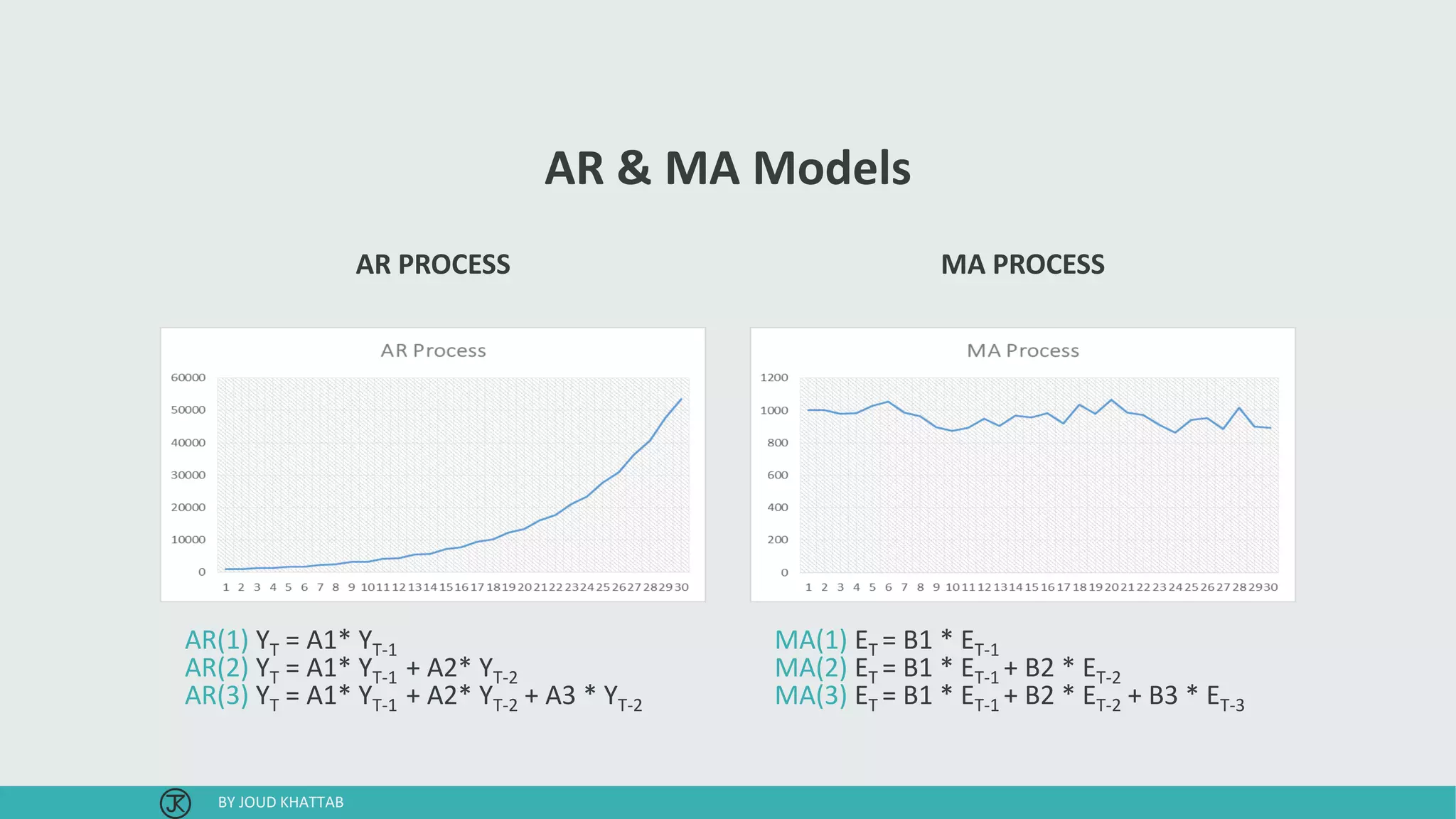
• Auto Regressive AR process:
• Series current values depend on its own previous values.
• AR(p) - Current values depend on its own p-previous values.
• P is the order of AR process.
• Moving Average MA process:
• The current deviation from mean depends on previous deviations.
• MA(q) - The current deviation from mean depends on q- previous deviations.
• q is the order of MA process.
• Autoregressive Moving average ARMA process.
BY JOUD KHATTAB

7. AR & MA Models
AR PROCESS MA PROCESS
AR(1) YT = A1* YT-1
AR(2) YT = A1* YT-1 + A2* YT-2
AR(3) YT = A1* YT-1 + A2* YT-2 + A3 * YT-2
MA(1) ΕT = B1 * ΕT-1
MA(2) ΕT = B1 * ΕT-1 + B2 * ΕT-2
MA(3) ΕT = B1 * ΕT-1 + B2 * ΕT-2 + B3 * ΕT-3
BY JOUD KHATTAB

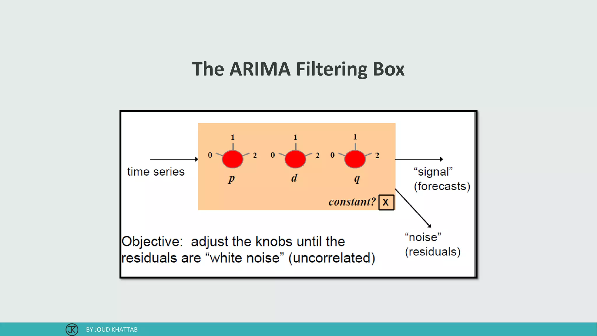
8. ARIMA (p,d,q) Modeling
• To build a time series model issuing ARIMA, we need to study the time series and
identify p,d,q.
1. Ensuring Stationarity:
• Determine the appropriate values of d.
2. Identification:
• Determine the appropriate values of p & q using the ACF, PACF.
3. Diagnostic checking:
• pick best model with well behaved residuals.
4. Forecasting:
• Produce out of sample forecasts or set aside last few data points for in-sample forecasting.
BY JOUD KHATTAB

9. Achieving Stationarity
• A stationary time series is one whose statistical properties such as mean, variance,
autocorrelation, etc. are all constant over time.
• Differencing: Transformation of the series to a new time series where the values are the
differences between consecutive values.
• Procedure may be applied consecutively more than once.
BY JOUD KHATTAB

10. Stationarity Example:
Avoiding Common Mistakes with Time Series
• A basic mantra in statistics and data science is correlation is not causation, meaning
that just because two things appear to be related to each other doesn’t mean that one
causes the other. This is a lesson worth learning.
BY JOUD KHATTAB

11. Stationarity Example:
Two Random Series
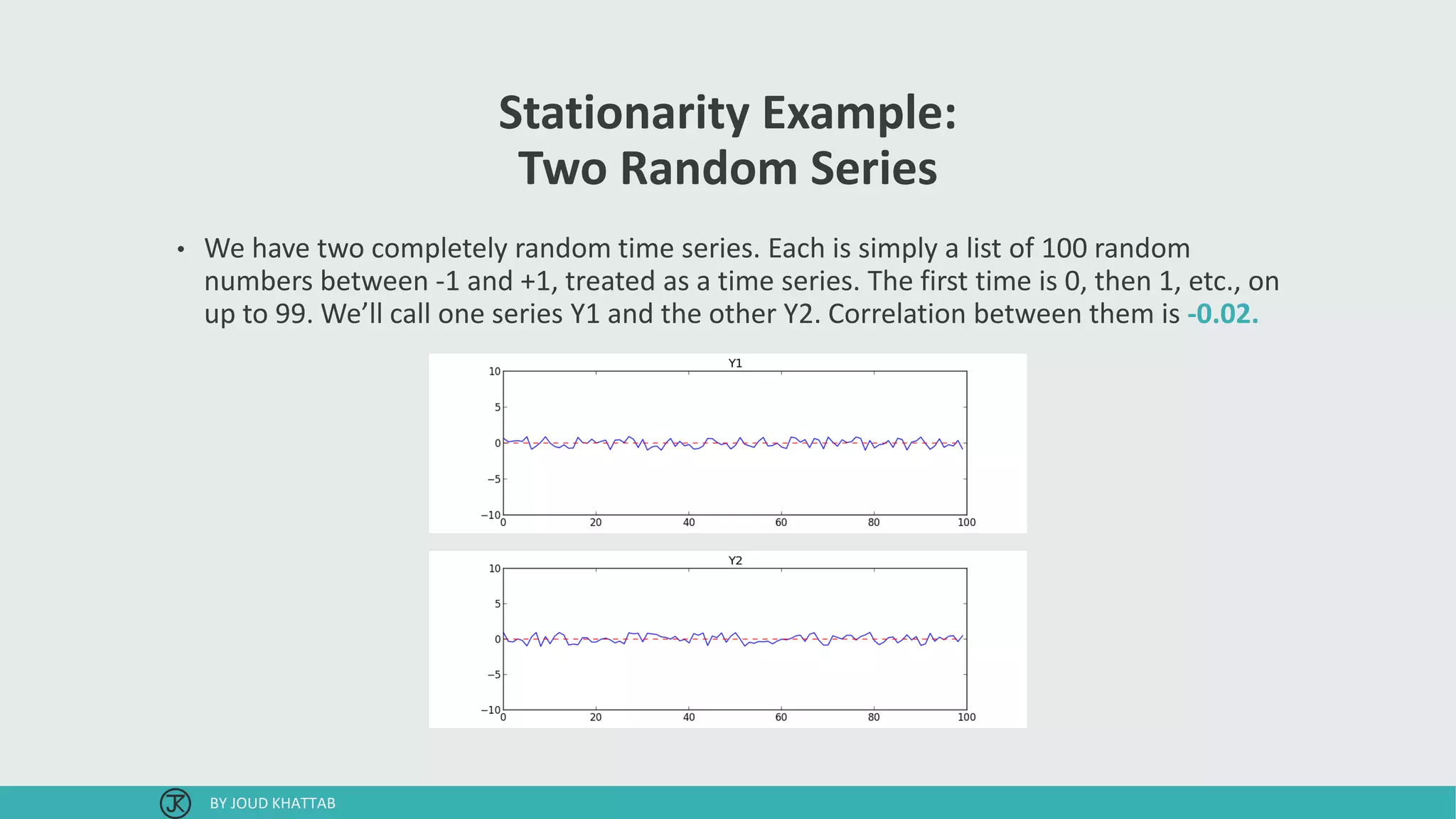
• We have two completely random time series. Each is simply a list of 100 random
numbers between -1 and +1, treated as a time series. The first time is 0, then 1, etc., on
up to 99. We’ll call one series Y1 and the other Y2. Correlation between them is -0.02.
BY JOUD KHATTAB

12. Stationarity Example:
Adding trend
• Now let’s tweak the time series by adding a slight rise to each. Specifically, to each
series we simply add points from a slightly sloping line from (0,-3) to (99,+3). Now let’s
repeat the same tests on these new series. We get surprising results: the correlation
coefficient is 0.96.
BY JOUD KHATTAB

13. Stationarity Example:
Dealing With Trend
• What’s going on? The two time series are no more related than before. By introducing a
trend, we’ve made Y1 dependent on X, and Y2 dependent on X as well. In a time series,
X is time. Correlating Y1 and Y2 will uncover their mutual dependence.
• One such method for removing trend is called first differences. With first differences,
you subtract from each point the point that came before it:
• y'(t) = y(t) – y(t-1)
BY JOUD KHATTAB

14. Differentiation
ACTUAL SERIES SERIES AFTER DIFFERENTIATION
BY JOUD KHATTAB

15. Identification “p” and “q” Orders
• We need to learn about ACF & PACF to identify p,q.
• Once we are working with a stationary time series, we can examine the ACF and PACF
to help identify the proper number of lagged y (AR) terms and ε (MA) terms.
BY JOUD KHATTAB

16. Autocorrelation Function (ACF)
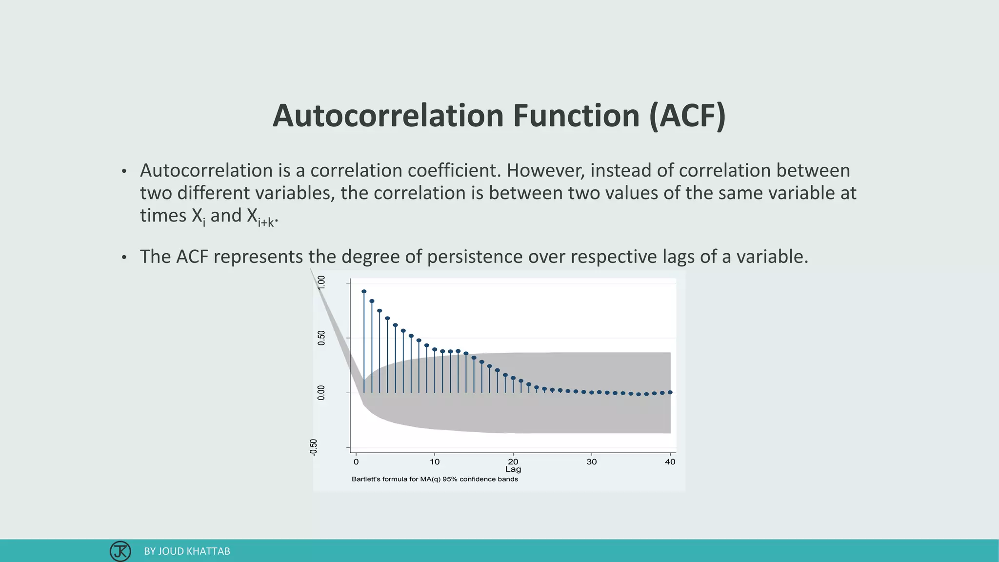
• Autocorrelation is a correlation coefficient. However, instead of correlation between
two different variables, the correlation is between two values of the same variable at
times Xi and Xi+k.
• The ACF represents the degree of persistence over respective lags of a variable.
-0.50
0.000.501.00
Autocorrelationsofpresap
0 10 20 30 40
Lag
Bartlett's formula for MA(q) 95% confidence bands
BY JOUD KHATTAB

17. Partial Autocorrelation Function (PACF)
• Partial correlation measures the degree of association between two random variables,
with the effect of a set of controlling random variables removed.
-0.50
0.000.501.00
Partialautocorrelationsofpresap
0 10 20 30 40
Lag
95% Confidence bands [se = 1/sqrt(n)]
BY JOUD KHATTAB

18. Identification of AR Processes & its order (p)
• For AR models, the ACF will dampen exponentially.
• The PACF will identify the order of the AR model:
• The AR(1) model would have one significant spike at lag 1 on the PACF.
• The AR(3) model would have significant spikes on the PACF at lags 1, 2, & 3.
-0.50
0.000.501.00
Autocorrelationsofpresap
0 10 20 30 40
Lag
Bartlett's formula for MA(q) 95% confidence bands
-0.50
0.000.501.00
Partialautocorrelationsofpresap
0 10 20 30 40
Lag
95% Confidence bands [se = 1/sqrt(n)]
BY JOUD KHATTAB

19. Identification of MA Processes & its order (q)
• The PACF will dampen exponentially.
• The ACF will be used to identify the order of the MA process.
• The MA(1) has one significant spike in the ACF at lag 1.
• The MA(3) has three significant spikes in the ACF at lags 1, 2, & 3.
-0.50
0.000.501.00
Autocorrelationsofpresap
0 10 20 30 40
Lag
Bartlett's formula for MA(q) 95% confidence bands
-0.50
0.000.501.00
Partialautocorrelationsofpresap
0 10 20 30 40
Lag
95% Confidence bands [se = 1/sqrt(n)]
BY JOUD KHATTAB

20. The ARIMA Filtering Box
BY JOUD KHATTAB

21. Seasonal ARIMA
BY JOUD KHATTAB

22. Seasonal Time Series
• A seasonal pattern exists when a series is influenced by seasonal factors (e.g., the
quarter of the year, the month, or day of the week). Seasonality is always of a fixed and
known period.
BY JOUD KHATTAB

23. Seasonal ARIMA
• A seasonal ARIMA model is formed by including additional seasonal terms in the
ARIMA models we have seen so far. It is written as follows:
• Where m = number of periods per season.
• We use uppercase notation for the seasonal parts of the model, and lowercase notation
for the non-seasonal parts of the model.
BY JOUD KHATTAB

24. Seasonal ARIMA
• The seasonal part consists of terms that are very similar to the non-seasonal
components of the model, but they involve backshifts of the seasonal period.
• For example, an ARIMA(1,1,1)(1,1,1)4 model is for quarterly data (m=4).
• The additional seasonal terms are simply multiplied with the non-seasonal terms.
BY JOUD KHATTAB

25. ACF & PACF
• The seasonal part of an AR or MA model will be seen in the seasonal lags of the PACF and
ACF.
• For example, an ARIMA(0,0,0)(0,0,1)12 model will show:
• A spike at lag 12 in the ACF but no other significant spikes.
• The PACF will show exponential decay in the seasonal lags; that is, at lags 12, 24, 36, ….
• Similarly, an ARIMA(0,0,0)(1,0,0)12 model will show:
• Exponential decay in the seasonal lags of the ACF.
• A single significant spike at lag 12 in the PACF.
• In considering the appropriate seasonal orders for an ARIMA model, restrict attention to the
seasonal lags.
• The modelling procedure is almost the same as for non-seasonal data, except that we need
to select seasonal AR and MA terms as well as the non-seasonal components of the model.
BY JOUD KHATTAB

26. The Filtering Box Now Has 6 Knobs
BY JOUD KHATTAB

27. SARIMA in R
(CASE STUDY)
BY JOUD KHATTAB

28. European Quarterly Retail Trade
• We will describe the seasonal ARIMA modelling procedure using quarterly European
retail trade data from 1996 to 2011.
• We will use Forecast Library in R studio.
plot(euretail, ylab="Retail index", xlab="Year")
BY JOUD KHATTAB

29. Make It Stationary
• The data are clearly non-stationary, with some seasonality, so we will first take a
seasonal difference.
tsdisplay( diff(euretail,4) )
BY JOUD KHATTAB

30. Make It Stationary
• These also appear to be non-stationary, and so we take an additional first difference.
tsdisplay( diff( diff(euretail,4) ) )
BY JOUD KHATTAB

31. Find Appropriate ARIMA Model
• Based on the ACF and PACF shown:
• The significant spike at lag 1 in the ACF
suggests a non-seasonal MA(1)
component.
• The significant spike at lag 4 in the ACF
suggests a seasonal MA(1) component.
• Consequently, we begin with an
ARIMA(0,1,1)(0,1,1)4 model, indicating
a first and seasonal difference, and
non-seasonal and seasonal MA(1)
components.
BY JOUD KHATTAB

32. Find Appropriate ARIMA Model
ARIMA(0,1,1)(0,1,1)4
• Both the ACF and PACF show significant
spikes at lag 2, and almost significant
spikes at lag 3, indicating some
additional non-seasonal terms need to
be included in the model.
• The AICc of:
• ARIMA(0,1,2)(0,1,1)4 model is 74.36.
• ARIMA(0,1,3)(0,1,1)4 model is 68.53.
• We tried other models with AR terms
as well, but none that gave a smaller
AICc value.
fit <- Arima(euretail, order=c(0,1,1), seasonal=c(0,1,1))
tsdisplay(residuals(fit))
BY JOUD KHATTAB

33. Find Appropriate ARIMA Model
ARIMA(0,1,3)(0,1,1)4
• All the spikes are now within the
significance limits, and so the residuals
appear to be white noise.
• A Ljung-Box test also shows that the
residuals have no remaining
autocorrelations.
fit3 <- Arima(euretail, order=c(0,1,3), seasonal=c(0,1,1))
res <- tsdisplay(residuals(fit3))
Box.test(res, lag=16, fitdf=4, type="Ljung")
BY JOUD KHATTAB

34. Forecast Model
• Forecasts from the model for the next
six years as shown.
• Notice how the forecasts follow the
recent trend in the data (this occurs
because of the double differencing).
• The large and rapidly increasing
prediction intervals show that the retail
trade index could start increasing or
decreasing at any time while the point
forecasts trend downwards.
plot( forecast(fit3, h=24) )
BY JOUD KHATTAB

35. Forecast Without Seasonality
fit <- Arima(euretail, order=c(1,2,0))
tsdisplay(residuals(fit))
plot(forecast(fit, h=24))
BY JOUD KHATTAB

36. Find Appropriate ARIMA Model
Other Method
• We could have used auto.arima() to do
most of this work for us. It would have
given the following result.
> auto.arima(euretail, stepwise=FALSE,
approximation=FALSE)
ARIMA(0,1,3)(0,1,1)[4]
Coefficients:
ma1 ma2 ma3 sma1
0.2625 0.3697 0.4194 -0.6615
s.e. 0.1239 0.1260 0.1296 0.1555
sigma^2 estimated as 0.1451: log likeliho
od=-28.7
AIC=67.4 AICc=68.53 BIC=77.78
BY JOUD KHATTAB

37. Thank You
BY JOUD KHATTAB