Downloaded 96 times
![ASU-CSC445: Neural Networks Prof. Dr. Mostafa Gadal-Haqq
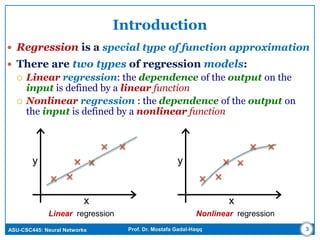
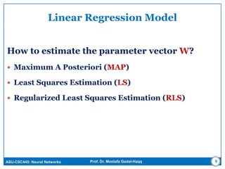
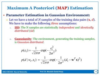
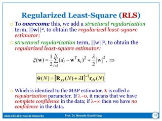
Linear Regression Model
Linear Regression (One variable)
The parameter vector w = [ w0 w1 ] is fixed but unknown;
stationary environment.
bay x
6
y
x
Linear regression
01 x wwy
a = slope
b = intercept](https://image.slidesharecdn.com/aw53cy0jrbyiqwb1mnop-signature-7f7e9932c1ac6134e9030bbdd4cfa1c5606f58d572ef5d7da58609957cc1fc67-poli-160617131027/85/Neural-Networks-Model-Building-Through-Linear-Regression-6-320.jpg)
![ASU-CSC445: Neural Networks Prof. Dr. Mostafa Gadal-Haqq
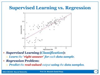
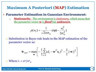
Linear Regression Model
Linear Regression (Multiple variables)
The parameter vector w is
fixed but unknown;
stationary environment.
Figure 2.1(a) Unknown stationary stochastic environment.
(b) Linear regression model of the environment.
M
j
jjxwd
1
xwT
d
7
T
Mxxx ],...,,[ 21x](https://image.slidesharecdn.com/aw53cy0jrbyiqwb1mnop-signature-7f7e9932c1ac6134e9030bbdd4cfa1c5606f58d572ef5d7da58609957cc1fc67-poli-160617131027/85/Neural-Networks-Model-Building-Through-Linear-Regression-7-320.jpg)
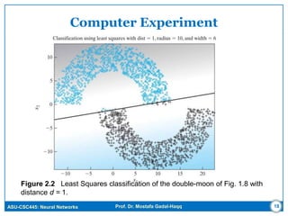
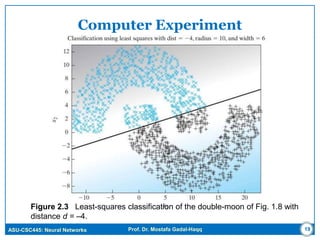


The document discusses regression models for modeling relationships between input and output variables. It covers linear regression, using linear functions to model the relationship, and nonlinear regression, using nonlinear functions. Maximum a posteriori (MAP) estimation and least squares estimation are described as approaches for estimating the parameters of regression models from data. MAP estimation maximizes the posterior probability of the parameters given the data and assumes prior probabilities on the parameters, while least squares minimizes error. Regularized least squares is also covered, which adds a regularization term to improve stability. Computer experiments are demonstrated applying linear regression to classification problems.