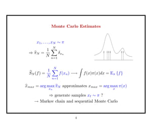
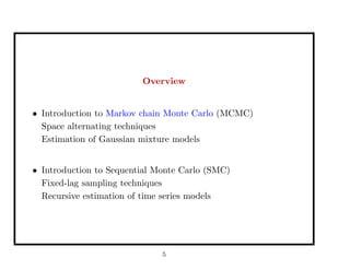
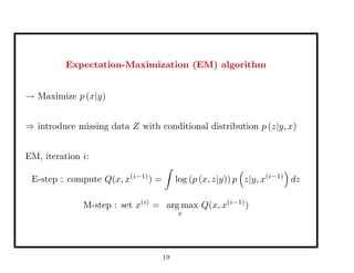
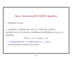
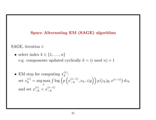
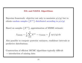
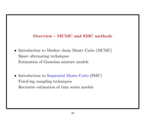
This document discusses recent advances in Markov chain Monte Carlo (MCMC) and sequential Monte Carlo (SMC) methods. It introduces Markov chain and sequential Monte Carlo techniques such as the Hastings-Metropolis algorithm, Gibbs sampling, data augmentation, and space alternating data augmentation. These techniques are applied to problems such as parameter estimation for finite mixtures of Gaussians.

1. Some recent advances in Markov chain and
sequential Monte Carlo methods
St´ephane S´en´ecal
The Institute of Statistical Mathematics,
Research Organization of Information and Systems
15/12/2004
thanks to the Japan Society for the Promotion of Science
1

2. Estimation
x
S=F(., )
b
y
θ
Information on (x, θ): distribution of probability
p(x, θ|y, F, prior ) ∝ p(y|x, θ, F, prior ) × p(x, θ|prior )
⇒ Estimates (x, θ)
2

3. Estimates
• Maximum a posteriori (MAP)
(x, θ) = arg max
x,θ
p(x, θ|y, prior )
• Expectation: posterior mean E {x, θ|y, prior}
Ep(.|y,prior ) {f(x, θ)} = f(x, θ)p(x, θ|y, prior )d(x, θ)
Computation : asymptotic, numerical, stochastic methods
⇒ Monte Carlo simulation methods
3

4. Monte Carlo Estimates
x1, . . . , xN ∼ π
⇒ πN =
1
N
N
n=1
δxn
SN (f) =
1
N
N
n=1
f(xn) −→ f(x)π(x)dx = Eπ {f}
xmax = arg max
xn
πN approximates xmax = arg max
x
π(x)
⇒ generate samples x ∼ π ?
→ Markov chain and sequential Monte Carlo
4

5. Overview
• Introduction to Markov chain Monte Carlo (MCMC)
Space alternating techniques
Estimation of Gaussian mixture models
• Introduction to Sequential Monte Carlo (SMC)
Fixed-lag sampling techniques
Recursive estimation of time series models
5

6. Simulation Techniques
• Classical distributions : cumulated density function
→ transformation of uniform random variable
• Non-standard distributions, Rn
, known up to a normalizing
constant → usage of instrumental distribution:
Accept-reject, importance sampling → sequential/recursive
⇒ SMC aka particle filtering, condensation algorithm
⇒ MCMC : distribution = fixed point of an operator
π = Kπ
→ simulation schemes with Markov chain: Hastings-Metropolis,
Gibbs sampling
6

7. Markov Chain
Definition:
Xn|Xn−1, Xn−2, . . . , X0
d
= Xn|Xn−1
homogeneity : Xn|Xn−1 independent of n
Realization:
X0 ∼ π0(x0)
p.d.f. of Xn|Xn−1 = transition kernel K(xn|xn−1)
7

8. Simulation of Markov chain
Convergence: Xn ∼ π asymptotically ?
π-invariance : π(.) = Kπ(.)
A
π(x)dx =
y∈A
K(y|x)π(x)dxdy
⇐ π-reversibility : Pr(A → B) = Pr(B → A)
y∈B x∈A
K(y|x)π(x)dxdy =
y∈A x∈B
K(y|x)π(x)dxdy
Construct kernels K(.|.) such that the chain is π-invariant
• Hastings-Metropolis algorithm
• Gibbs sampling
8

9. Hastings-Metropolis
Draw x from π(.)
1. initialize x0 ∼ π0(x)
2. Iteration
• propose candidate x for x +1 → x ∼ q(x|x )
• accept it with prob α = min{1, r}
3. ← + 1 and go to (2)
r =
π(x )q(x |x )
q(x |x )π(x )
→ π(x)K(y|x) = π(y)K(x|y)
π(x)q(y|x) min 1,
π(y)q(x|y)
q(y|x)π(x)
= min {π(x)q(y|x), π(y)q(x|y)}
q(x |x ) = q(x ) q(x |x ) = q(|x − x |)
9

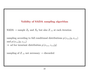
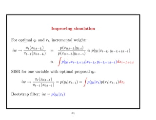
10. Example
sample x ∼ p(x) ∝ 1
1+x2 20,000 iterations
x ∼ N(x , 0.12
)
0 0.2 0.4 0.6 0.8 1 1.2 1.4 1.6 1.8 2
x 10
4
−5
0
5
10
15
−6 −4 −2 0 2 4 6 8 10 12 14
0
0.1
0.2
0.3
0.4
0.5
0.6
0.7
acc. rate = 97%
x ∼ U[a,b]
0 0.2 0.4 0.6 0.8 1 1.2 1.4 1.6 1.8 2
x 10
4
−15
−10
−5
0
5
10
15
−15 −10 −5 0 5 10 15
0
0.1
0.2
0.3
0.4
0.5
0.6
0.7
acc. rate = 26%
10

11. Gibbs sampling algorithm
Sample x = (x1, ...xp) ∼ π(x1, ...xp)
1. initialize x(0)
∼ π0(x), = 0
2. iteration : Sample
x
( +1)
1 ∼ π1(x1|x
( )
2 , . . . , x( )
p )
x
( +1)
2 ∼ π2(x2|x
( +1)
1 , x
( )
3 , . . . , x( )
p )
...
x( +1)
p ∼ πp(xp|x
( +1)
1 , . . . , x
( +1)
p−1 )
3. ← + 1 and go to (2)
→ no rejection, reversible kernel
11

12. x =


x1
x2

 ∼ N




0
0

 ,


1 ρ
ρ 1




x
( +1)
1 |x
( )
2 ∼ N ρx
( )
2 , 1 − ρ2
x
( +1)
2 |x
( +1)
1 ∼ N ρx
( +1)
1 , 1 − ρ2
−4 −3 −2 −1 0 1 2 3 4
−4
−3
−2
−1
0
1
2
3
4
x1
x2
5,000 samples, ρ=0.5
−6 −4 −2 0 2 4 6
0
1000
2000
3000
4000
5000
6000
7000
8000
9000
−6 −4 −2 0 2 4 6
0
1000
2000
3000
4000
5000
6000
7000
8000
9000
histograms (x1, x2)
12

13. How to obtain fast converging simulation scheme ?
→ Missing Data, Data Augmentation, Latent Variables
Idea : extend sampling space x → (x, z) and distribution
π(x) → π(x, z) with constraint
π(x, z)dz = π(x)
such that Markov chain (x(i)
, z(i)
) ∼ π faster
• Optimization : Expectation-Maximization (EM) algorithm
• Simulation : Data Augmentation, Gibbs sampling
13

14. Efficient Data Augmentation Schemes
Idea: construct missing data space as less informative as possible
x
pi(x)
x ∼ π(x)
x
pitilde(x,z) = constant
z
(x, z) ∼ π(x, z)
Information introduced in missing data : convergence
14

15. Efficient Data Augmentation Schemes
EM algorithm → Space Alternating Generalized EM
SAGE algorithm, Hero and Fessler 1994:
• update parameter components by subblocks
• specific missing data space associated with each subblock
• complete data spaces less informative → convergence rate
15

16. Efficient Data Augmentation Sampling Schemes
SAGE Idea → MCMC algorithm:
• sample parameter components by subblocks
• each subblock of parameters is sampled conditionaly on a specific
missing data set
⇒ Space Alternating Data Augmentation (SADA)
A. Doucet, T. Matsui, S. S´en´ecal 2004
• Optimization : EM algorithm → SAGE algorithm
• Simulation : DA, Gibbs sampling → SADA
16

17. Overview - Space alternating techniques
• → Introduction to EM and SAGE algorithms
• Introduction to Data Augmentation and SADA algorithms
• Application to Finite Mixture of Gaussians
17

18. EM and SAGE Algorithms
Bayesian framework: obtaining MAP estimate of random variable X
given realization of Y = y
xMAP = arg max p (x|y)
where
p (x|y) ∝ p (y|x) p (x)
X is random vector whose components are partitioned into n subsets
X = X1:n = (X1, . . . , Xn)
Notation X−k = X1:n {Xk} = (X1, . . . , Xk−1, Xk+1, . . . , Xn) and
Zk:j = (Zk, Zk+1, . . . , Zj)
18

19. Expectation-Maximization (EM) algorithm
→ Maximize p (x|y)
⇒ introduce missing data Z with conditional distribution p (z|y, x)
EM, iteration i:
E-step : compute Q(x, x(i−1)
) = log (p (x, z|y)) p z|y, x(i−1)
dz
M-step : set x(i)
= arg max
x
Q(x, x(i−1)
)
19

20. Space Alternating EM (SAGE) algorithm
→ Maximize p (x|y)
⇒ introduce n missing data sets Z1:n with each random
variable/vector Zk is given a conditional distribution p (zk|y, x1:n)
satisfying
p (y|x1:n, zk) = p (y|x−k, zk)
→ zk independent of xk conditionaly on x−k and y
→ non-informative missing data space
20

21. Space Alternating EM (SAGE) algorithm
SAGE, iteration i:
• select index k ∈ {1, . . . , n}
e.g. components updated cyclically k = (i mod n) + 1
• EM step for computing x
(i)
k :
set x
(i)
k = arg max
x
log p x
(i−1)
−k , xk, z|y p zk|y, x(i−1)
dzk
and set x
(i)
−k = x
(i−1)
−k
21

22. DA and SADA Algorithms
Bayesian framework: objective not only to maximize p (x|y) but to
obtain random samples X(i)
distributed according to p (x|y)
Based on samples X(i)
, approximation of MMSE estimate:
xMMSE =
1
N
N
i=1
X(i)
→ xMMSE = xp (x|y) dx
Also possible to compute posterior variances, confidence intervals or
predictive distributions.
Construction of efficient MCMC algorithms typically difficult
→ introduction of missing data
22

23. Data Augmentation, Gibbs sampling
→ Sample p (x|y)
⇒ introduce missing data Z with joint posterior distribution
p (x, z|y) = p (x|y) p (z|y, x)
Data Augmentation algorithm, iteration i given X(i−1)
:
• Sample Z(i)
∼ p ·|y, X(i−1)
• Sample X(i)
∼ p ·|y, Z(i)
23

24. Convergence of DA/Gibbs sampling algorithm
• Transition kernel associated to X(i)
, Z(i)
admits p (x, z|y) as
invariant distribution
• Under weak additional assumptions
(irreducibility and aperiodicity)
instantaneous distribution of X(i)
, Z(i)
converges towards
p (x, z|y) as i → +∞
24

25. Space Alternating Data Augmentation
→ Sample p (x|y)
⇒ introduce n missing data sets Z1:n with each random variable Zk
is given a conditional distribution p (zk|y, x1:n) such that
p (y|x1:n, zk) = p (y|x−k, zk)
→ zk independent of xk conditionaly on x−k and y
→ non-informative missing data space
Sampling of joint posterior distribution:
p (x1:n, z1:n|y) = p (x1:n|y)
n
k=1
p (zk|y, x1:n)
25

26. Space Alternating Data Augmentation
SADA algorithm, iteration i
given X
(i−1)
1:n and component index k:
• Sample Z
(i)
k ∼ p ·|y, X(i−1)
• Sample X
(i)
k ∼ p ·|y, Z
(i)
k , X
(i−1)
−k
• Set X
(i)
−k = X
(i−1)
−k
Components updated cyclically k = (i mod n) + 1
26

27. Validity of SADA sampling algorithm
Generation of Markov chain X
(i)
1:n, Z
(i)
1:n with invariant distribution
p (x1:n, z1:n|y)
Idea: SADA equivalent to
• Sample Z
(i)
k , Z−k ∼ p ·|y, X
(i−1)
1:n
• Sample X
(i)
k , Z−k ∼ p ·|y, Z
(i)
k , X
(i−1)
−k
• Set X
(i)
−k = X
(i−1)
−k
27

28. Validity of SADA sampling algorithm
SADA → sample Zk and Xk but also Z−k at each iteration
sampling according to full conditional distributions p (z1:n|y, x1:n)
and p (x1:n|y, z1:n)
⇒ ad hoc invariant distribution p (x1:n, z1:n|y)
sampling of Z−k not necessary → discarded
28

29. Overview - Space alternating techniques
• Introduction to EM and SAGE algorithms
• Introduction to Data Augmentation and SADA algorithms
• ⇒ Application to Finite Mixture of Gaussians
29

30. Finite Mixture of Gaussians
EM/DA algorithms routinely used to perform ML/MAP parameter
estimation/to sample the posterior distribution
Straightforward extensions to hidden Markov chains with Gaussian
observations
T i.i.d. observations Y1:T in Rd
, distributed according to a finite
mixture of s Gaussians
Yt ∼
s
j=1
πjN (µj; Σj)
30

31. Bayesian Estimation
Parameters
X = {(µj, Σj, πj) ; j = 1, . . . , s}
unknown, random, distributed from conjugate prior distributions
µj|Σj ∼ N (αj, Σj/λj)
Σ−1
j ∼ W (rj, Cj)
(π1, . . . , πs) ∼ D (ζ1, . . . , ζs)
31

32. Bayesian Estimation
Σ−1
∼ W (r, C): Wishart distribution, p.d.f. proportional to
|Σ−1
|
1
2 (r−d−1)
exp −
1
2
tr Σ−1
C−1
(π1, . . . , πs) ∼ D (ζ1, . . . , ζs): Dirichlet distribution restricted to the
simplex, p.d.f. proportional to
s
k=1 πζk−1
k
Hyperparameters {(αj, λj, rj, Cj, ζj) ; j = 1, . . . , s} assumed fixed but
could be estimated from data in a hierarchical Bayes model
32

33. Missing Data for Finite Mixture of Gaussians
EM/DA introduce the i.i.d. missing data Zt ∈ {1, . . . , s} such that
Yt|Zt = j ∼ N (µj; Σj)
Pr (Zt = j) = πj
Gibbs sampling algorithm, iteration i:
• sample discrete latent variables Z
(i)
t ∼ p ·|yt, X(i−1)
• compute sufficient statistics n
(i)
j
T
t=1 δZ
(i)
t ,j
,
n
(i)
j y
(i)
j
T
t=1 δZ
(i)
t ,j
yt and S
(i)
j
T
t=1 δZ
(i)
t ,j
ytyT
t
• sample parameters
33

34. Gibbs sampling for Finite Mixture of Gaussians
sampling parameters, iteration i:
Σ
−1(i)
j ∼ W rj + n
(i)
j , Σ
−1(i)
j
µ
(i)
j |Σ
(i)
j ∼ N m
(i)
j ,
Σ
(i)
j
λj + n
(i)
j
π
(i)
1 , . . . , π(i)
s ∼ D n
(i)
1 + ζ1, . . . , n(i)
s + ζs
m
(i)
j =
λjαj + n
(i)
j y
(i)
j
λj + n
(i)
j
Σ
(i)
j = C−1
j + λjαjαT
j + S
(i)
j − λj + n
(i)
j m
(i)
j m
(i)T
j
34

35. Less Informative Missing Data
update only µj, τ2
j , µ−j, τ2
−j fixed
→ binary missing data Zt,j ∈ {0, j} such that Pr (Zt,j = j) = πj
variable Zt,j = “observation coming from component j or not”, less
informative than knowing “from which particular component
observation is derived”
constraint
s
j=1 πj = 1 ⇒ cannot update πj, use of standard EM
approach for sampling the weights
35

36. Less Informative Missing Data
→ updating jointly the parameters of two components j and k
(A. Doucet, T. Matsui and S. S´en´ecal, 2004)
→ missing data Zt,j,k ∈ {0, j, k} such that
Pr (Zt,j,k = j) = πj, Pr (Zt,j,k = k) = πk
and
Yt|Zt,j,k = j ∼ N (µj; Σj)
Yt|Zt,j,k = k ∼ N (µk; Σk)
Yt|Zt,j,k = 0 ∼
l=j,l=k πlN (µl; Σl)
l=j,l=k πl
36

37. SAGE algorithm for Finite Mixture of Gaussians
update for µj, τ2
j , iteration i:
µ
(i)
j =
λjαj +
T
t=1 ytp Zt,j,k = j|yt, X(i−1)
λj +
T
t=1 p Zt,j,k = j|yt, X(i−1)
Σ
(i)
j =
C−1
j + λj µ
(i)
j − αj µ
(i)
j − αj
T
+ . . .
. . .
. . . +
T
t=1
yt − µ
(i)
j yt − µ
(i)
j
T
p Zt,j,k = j|yt, X(i−1)
rj − d − 1 + λj +
T
t=1
p Zt,j,k = j|yt, X(i−1)
37

38. SAGE algorithm for Finite Mixture of Gaussians
update for πj, iteration i:
π
(i)
j =
1 − l=j,l=k π
(i−1)
l
1 +
T
t=1
p(Zt,j,k=k|yt,X(i−1)
)+(ζk−1)
T
t=1
p(Zt,j,k=j|yt,X(i−1)
)+(ζj −1)
π
(i)
k = 1 − π
(i)
j −
l=j,l=k
π
(i−1)
l
38

39. SADA algorithm for Finite Mixture of Gaussians
SADA algorithm, iteration i, sample (µj, Σj, πj)
• sample discrete latent variables
Z
(i)
t,j,k ∼ p ·|yt, X(i−1)
• compute sufficient statistics n
(i)
j
T
t=1 δZ
(i)
t,j,k,j
and
n
(i)
j y
(i)
j
T
t=1
δZ
(i)
t,j,k,j
yt, S
(i)
j
T
t=1
δZ
(i)
t,j,k,j
ytyT
t
• sample parameters
39

40. SADA algorithm for Finite Mixture of Gaussians
sampling parameters, iteration i:
Σ
−1(i)
j ∼ W rj + n
(i)
j , Σ
−1(i)
j
µ
(i)
j |Σ
(i)
j ∼ N m
(i)
j ,
Σ
(i)
j
λj + n
(i)
j
π
(i)
j , π
(i)
k ∼

1 −
l=j,l=k
π
(i−1)
l

 D n
(i)
j + ζj, n
(i)
k + ζk
40

41. Numerical experiments
Mixture of s = 8 d = 10-dimensional Gaussians
T = 100 samples
Parameters of components sampled from prior with parameters
ζj = 1, αj = 0, λj = 0.01, rj = d + 1 and Cj = 0.01I
100 iterations of EM and SAGE algorithms
41

42. Numerical experiments - s = 8 d = 10
0 5 10 15 20 25 30 35 40 45 50
−2000
−1800
−1600
−1400
−1200
−1000
−800
−600
−400
Log of posterior p.d.f. values (straight EM/dotted SAGE) / iterations
42

43. Numerical experiments - s = 5 d = 25
0 5 10 15 20 25 30 35 40 45 50
−5000
−4500
−4000
−3500
−3000
−2500
−2000
−1500
−1000
−500
0
Log of posterior p.d.f. values (straight EM/dotted SAGE) / iterations
43

44. Simulations
Mixture of s = 5 d = 10-dimensional Gaussians T = 100, parameters
of components sampled from prior with parameters ζj = 1, αj = 0,
λj = 0.01, rj = d + 1 and Cj = 0.01I
200 iterations of EM and SAGE 50 times
5000 iterations of DA and SADA 10 times
Results:
• EM/SAGE: mean of log-posterior values at final iteration
• SA/SADA: mean of average log-posterior values of last 1000
iterations
44

45. Simulations Results
s EM SAGE DA SADA
5 -915.8 -671.5 -873.7 -886.0
6 -929.6 –603.2 -877.3 -886.7
7 -941.4 -576.5 -893.9 -906.9
8 -965.7 -559.2 -904.9 -875.0
9 -968.9 -503.0 -898.8 -882.5
10 -983.2 -478.1 -924.0 -906.6
Log-posterior values for final iteration EM/SAGE
and average log-posterior values for DA/SADA
45

46. Conclusion - Perspectives
• Sampling complex distributions: MCMC → Hastings-Metropolis,
Gibbs sampler
• Speed-up convergence of optimisation/simulation algorithms:
missing data, data augmentation, latent/extended variable
→ space alternating techniques, non-informative data spaces
• Applications in modeling/estimation: speech processing,
tomography, digital communication, . . .
46

47. References - EM/SAGE/MCMC
• G. J. McLachlan and T. Krishnan, The EM Algorithm and
Extensions, Wiley Series in Probability and Statistics, 1997
• J. A. Fessler and A. O. Hero, Space-alternating generalized
expectation-maximization algorithm, IEEE Trans. Sig. Proc.,
42:2664–2677, 1994
• C. P. Robert and G. Casella, Monte Carlo Statistical Methods,
Springer-Verlag, 1999
• A. Doucet, T. Matsui and S. S´en´ecal, Space Alternating Data
Augmentation, ICASSP’05, 2005
47

48. Overview - MCMC and SMC methods
• Introduction to Markov chain Monte Carlo (MCMC)
Space alternating techniques
Estimation of Gaussian mixture models
• Introduction to Sequential Monte Carlo (SMC)
Fixed-lag sampling techniques
Recursive estimation of time series models
48

49. Estimation of state space models
xt = ft(xt−1, ut) yt = gt(xt, vt)
p(x0:t|y1:t) → p(xt|y1:t) = p(x0:t|y1:t)dx0:t−1
distribution of x0:t ⇒ computation of estimate x0:t:
x0:t = x0:tp(x0:t|y1:t)dx0:t → Ep(.|y1:t){f(x0:t)}
x0:t = arg max
x0:t
p(x0:t|y1:t)
49

50. Computation of the estimates
p(x0:t|y1:t) ⇒ multidimensionnal, non-standard distributions:
→ analytical, numerical approximations
→ integration, optimisation methods
⇒ Monte Carlo techniques
50

51. Monte Carlo approach
compute estimates for distribution π(.) → samples x1, . . . , xN ∼ π
x
pi(x)
x_1 x_N
⇒ distribution πN = 1
N
N
i=1 δxi approximates π(.)
51

52. Monte Carlo estimates
SN (f) =
1
N
N
i=1
f(xi) −→ f(x)π(x)dx = Eπ{f(x)}
arg max(xi)1≤i≤N
πN (xi) approximates arg maxx π(x)
⇒ sampling xi ∼ π difficult
→ importance sampling techniques
52

53. Simulation Techniques
• Classical distributions : cumulated density function
→ transformation of uniform random variable
• Non-standard distributions, Rn
, known up to a normalizing
constant → usage of instrumental distribution:
Accept-reject, importance sampling → sequential/recursive
⇒ SMC aka particle filtering, condensation algorithm
⇒ MCMC : distribution = fixed point of an operator, Markov
chain → simulation schemes: Hastings-Metropolis, Gibbs
sampling
53

54. Importance Sampling
xi ∼ π → candidate/proposal distribution xi ∼ g
x
g(x)
pi(x)
x_Nx_1
54

55. Importance Sampling
xi ∼ g = π → (xi, wi) weighted sample
⇒ weight wi =
π(xi)
g(xi)
x
g(x)
pi(x)
x_Nx_1
55

56. Estimation
importance sampling → computation of Monte Carlo estimates
e. g. expectations Eπ{f(x)}:
f(x)
π(x)
g(x)
g(x)dx = f(x)π(x)dx
N
i=1
wif(xi) → f(x)π(x)dx = Eπ{f(x)}
dynamic model (xt, yt) ⇒ recursive estimation x0:t−1 → x0:t
Monte Carlo techniques ⇒ sampling sequences x
(i)
0:t−1 → x
(i)
0:t
56

57. Sequential simulation
sampling sequences x
(i)
0:t ∼ πt(x0:t) recursively:
time
variable
state
x
p(x,t) target distribution:
t
t2
t1
p(x,t2)
x_t1
x_t2
p(x_t1)
p(x_t2)
p(x,t1)
57

58. Sequential simulation: importance sampling
samples x
(i)
0:t ∼ πt(x0:t) approximated by weighted particles
(x
(i)
0:t, w
(i)
t )1≤i≤N
time
p(x,t) target distribution:
p(x,t2)
t
t2
t1
x
p(x,t1)
58

59. Sequential importance sampling
diffusing particles x
(i)
0:t1
→ x
(i)
0:t2
time
p(x,t) target distribution:
p(x,t2)
t
x
p(x,t1)
t2
t1
⇒ sampling scheme x
(i)
0:t−1 → x
(i)
0:t
59

60. Sequential importance sampling
updating weights w
(i)
t1
→ w
(i)
t2
time
p(x,t) target distribution:
p(x,t2)
t
p(x,t1)
x
t2
t1
⇒ updating rule w
(i)
t−1 → w
(i)
t
60

61. Sequential Importance Sampling
x0:t ∼ πt(x0:t) ⇒ (x
(i)
0:t, w
(i)
t )1≤i≤N
Simulation scheme t − 1 → t:
• Sampling step x
(i)
t ∼ qt(xt|x
(i)
0:t−1)
• Updating weights
w
(i)
t ∝ w
(i)
t−1 ×
πt(x
(i)
0:t−1, x
(i)
t )
πt−1(x
(i)
0:t−1)qt(x
(i)
t |x
(i)
0:t−1)
incremental weight (iw)
normalizing
N
i=1 w
(i)
t = 1
61

62. Sequential Importance Sampling
x0:t ∼ πt(x0:t) ⇒ (x
(i)
0:t, w
(i)
t )1≤i≤N
proposal + reweighting →
pi(x_t)
x_t
62

63. Sequential Importance Sampling
proposal + reweighting → var{(w
(i)
t )1≤i≤N } with t
x_t
pi(x_t)
→ w
(i)
t ≈ 0 for all i except one
63

64. ⇒ Resampling
x_t
pi(x_t)
0 x_t^(1)
x_t^(j)1x_t^(i)2 x_t^(k)3
x_t^(N)0
→ draw N particles paths from the set (x
(i)
0:t)1≤i≤N
with probability (w
(i)
t )1≤i≤N
64

65. Sequential Importance Sampling/Resampling
Simulation scheme t − 1 → t:
• Sampling step x
,(i)
t ∼ qt(x,
t|x
(i)
0:t−1)
• Updating weights w
(i)
t ∝ w
(i)
t−1 ×
πt(x
(i)
0:t−1,x
,(i)
t )
πt−1(x
(i)
0:t−1)qt(x
,(i)
t |x
(i)
0:t−1)
→ parallel computing
• ⇒ Resampling step: sample N paths from (x
(i)
0:t−1, x
,(i)
t )1≤i≤N
→ particles interacting : computation at least O(N)
65

66. FV: Sequential simulation: SISR
Recursive estimation of state space models.
Approximation with particles, importance sampling.
time
x
p_t(x)
t
t+1
Bootstrap, particle filtering
Gordon et al. 1993, Kitagawa 1996, Doucet et al. 2001
→ time series, tracking.
66

67. FV: Sequential Importance Sampling/Resampling
Samples x
(i)
0:t ∼ πt(x0:t) approximated by
weighted particles (x
(i)
0:t, w
(i)
t )1≤i≤N
Simulation scheme t − 1 → t:
• Sampling step x
,(i)
t ∼ qt(x,
t|x
(i)
0:t−1)
• Updating weights w
(i)
t ∝ w
(i)
t−1 ×
πt(x
(i)
0:t−1, x
,(i)
t )
πt−1(x
(i)
0:t−1)qt(x
,(i)
t |x
(i)
0:t−1)
incremental weight (iw)
• Resampling step: sample N paths from (x
(i)
0:t−1, x
,(i)
t )1≤i≤N
67

68. SISR for recursive estimation of state space models
xt = ft(xt−1, ut) → p(xt|xt−1)
yt = gt(xt, vt) → p(yt|xt)
Usual SISR: Bootstrap filter (Gordon et al. 93, Kitagawa 96):
• Sampling step x
(i)
t ∼ p(xt|x
(i)
t−1)
• Updating weights : incremental weight w
(i)
t ∝ w
(i)
t−1 × iw
iw ∝ p(yt|x
(i)
t )
• Stratified/Deterministic resampling
efficient, easy, fast for a wide class of models
tracking, time series → nonlinear non-Gaussian state spaces
68

69. Improving simulation
Optimal proposal distribution qt(xt|x
(i)
0:t−1)
→ mimimizing variance of incremental weight (w
(i)
t ∝ w
(i)
t−1 × iw)
iw =
πt(x
(i)
0:t−1, x
(i)
t )
πt−1(x
(i)
0:t−1)qt(x
(i)
t |x
(i)
0:t−1)
⇒ 1-step ahead predictive:
πt(xt|x0:t−1) = p(xt|xt−1, yt)
⇒ incremental weight:
iw →
πt(x0:t−1)
πt−1(x0:t−1)
=
p(x0:t−1|y1:t)
p(x0:t−1|y1:t−1)
∝ p(yt|xt−1) = p(yt|xt)p(xt|xt−1)dxt
69

70. Improving simulation
sampling/approximating predictive πt(xt|x0:t−1) may not be efficient
for diffusing particles: e.g. discrepancy (πt)t>0 high:
⇒ consider a block of variables xt−L:t for a fixed lag L
70

71. Approaches using a block of variables
• discrete distributions, Meirovitch 1985
• auxiliary variables, Pitt and Shephard 1999
• reweighting before resampling, Wang et al. 2002
⇒ discrete distribution → analytical form for
xt ∼ πt+L(xt|x0:t−1) = πt+L(xt:t+L|x0:t−1)dxt+1:t+L
Meirovitch 1985: random walk in discrete space (growing a polymer)
→ complexity X L
for lag L
71

72. Reweighting + resampling
2
1
01
0
0
0
0
1 1
72

73. Reweighting
→ need to sample xt by block
⇒ design a proposal/candidate distribution
73

74. Sampling recursively a block of variables
t−L t−L+1 tt−1
xt−L:t−1 → xt−L+1:t: imputing xt and re-imputing xt−L+1:t−1
74

75. Sampling a block of variables
t−L t−L+1 tt−1
t−L+1x’(
t−L+1x(
0
:0 t−1x(
:0 t−Lx(
:t)
)
)
)t−1:
Proposal/candidate distribution for the “natural” block:
(x0:t−L, xt−L+1:t) ∼ πt−1(x0:t−1)qt(xt−L+1:t|x0:t−1)dxt−L+1:t−1
75

76. Sampling a block of variables
t−L t−L+1 tt−1
t−L+1x’(
t−L+1x(
0
:0 t−1x(
:0 t−Lx(
:t)
)
)
)t−1:
Candidate distribution for the extended block:
(x0:t−L, xt−L+1:t) → (x0:t−L, xt−L+1:t−1, xt−L+1:t) :
(x0:t−1, xt−L+1:t) ∼ πt−1(x0:t−1)qt(xt−L+1:t|x0:t−1)
76

77. Sampling a block of variables
Target distribution for the “natural” block (x0:t−L, xt−L+1:t):
πt(x0:t−L, xt−L+1:t)
⇒ auxiliary target distribution for the extended block
(x0:t−1, xt−L+1:t) = (x0:t−L, xt−L+1:t−1, xt−L+1:t) :
πt(x0:t−L, xt−L+1:t)rt(xt−L+1:t−1|x0:t−L, xt−L+1:t)
with rt = any conditional distribution
⇒ proposal + target distributions → importance sampling
77

78. Fixed-Lag Sequential Monte Carlo
A. Doucet and S. S´en´ecal, 2004
Simulation scheme t − 1 → t (index (i) dropped):
• Sampling step
xt−L+1:t ∼ qt(xt−L+1:t|x0:t−1)
• Updating weights
wt ∝ wt−1 ×
πt(x0:t−L, xt−L+1:t)rt(xt−L+1:t−1|x0:t−L, xt−L+1:t)
πt−1(x0:t−1)qt(xt−L+1:t|x0:t−1)
• Resampling step
78

79. Improving simulation
Optimal proposal distribution qt(xt−L+1:t|x0:t−1):
→ mimimizing variance of incremental weight:
iw =
πt(x0:t−L, xt−L+1:t)rt(xt−L+1:t−1|x0:t−L, xt−L+1:t)
πt−1(x0:t−1)qt(xt−L+1:t|x0:t−1)
⇒ qt = L-step ahead predictive
πt(xt−L+1:t|x0:t−L) = p(xt−L+1:t|xt−L, yt−L+1:t)
For one variable: optimal qt = 1-step ahead predictive
πt(xt|x0:t−1) = p(xt|xt−1, yt)
79

80. Improving simulation
Mimimizing variance of incremental weight
⇒ optimal target distribution
iw =
πt(x0:t−L, xt−L+1:t)rt(xt−L+1:t−1|x0:t−L, xt−L+1:t)
πt−1(x0:t−1)qt(xt−L+1:t|x0:t−1)
→ optimal conditional distribution rt(xt−L+1:t−1|x0:t−L, xt−L+1:t)
⇒ rt = (L − 1)-step ahead predictive
πt−1(xt−L+1:t−1|x0:t−L) = p(xt−L+1:t−1|xt−L, yt−L+1:t−1)
80

81. Improving simulation
For optimal qt and rt, incremental weight:
iw →
πt(x0:t−L)
πt−1(x0:t−L)
=
p(x0:t−L|y1:t)
p(x0:t−L|y1:t−1)
∝ p(yt|xt−L, yt−L+1:t−1)
∝ p(yt, xt−L+1:t|xt−L, yt−L+1:t−1)dxt−L+1:t
SISR for one variable with optimal proposal qt:
iw →
πt(x0:t−1)
πt−1(x0:t−1)
= p(yt|xt−1) = p(yt|xt)p(xt|xt−1)dxt
Bootstrap filter: iw = p(yt|xt)
81

82. Example
Nonlinear state space model:
xt = α(xt−1 + βx3
t−1) + ut x0, ut ∼ N(0, σ2
u)
yt = xt + vt vt ∼ N(0, σ2
v)
Sequential Monte Carlo methods:
• Bootstrap filter, proposal p(xt|xt−1)
• SISR with optimal proposal p(xt|xt−1, yt)
• SISR for blocks with optimal proposal p(xt−L+1:t|xt−L, yt−L+1:t)
approximated by forward-backward recursions with KF/EKF
Parameters values α=0.9, β=0.4, σu=0.1 and σv=0.05
⇒ approximation of target distribution p(xt|y1:t)
82

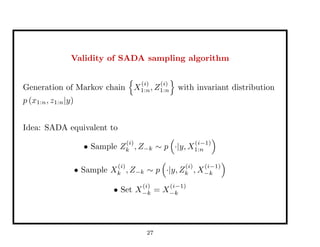
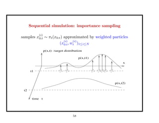
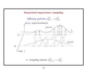
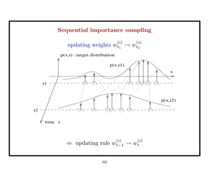
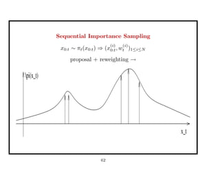
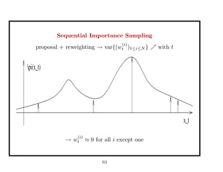
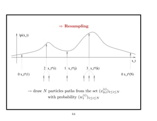
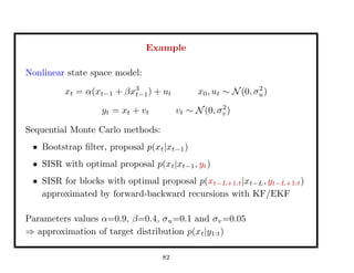
83. Approximation of the target distribution
⇒ Effective Sample Size:
ESS =
1
N
i=1[w
(i)
t ]2
w(i)
= 1
N : ESS = N
pi(x_t)
x_t
w(i)
≈ 0 ∀i except one: ESS = 1
x_t
pi(x_t)
⇒ Resampling performed for ESS ≤ N
2 , N
10
83

84. Simulation results
algorithm MSE ESS RS CPU
Bootstrap 0.0021 36.8 70.3 % 0.68
SISR 0.0019 65.8 19.2% 0.48
BSISR-KF 0.0018 72.3 0.9% 0.21
BSISR-EKF 0.0018 73.5 0.8% 0.24
N = 100 particles, 100 runs of particle filters for a single and for a
block of L = 2 variables.
84

85. Approximation of the target distribution
Resampling for ESS ≤ N
2 , N = 100
0 20 40 60 80 100 120 140 160 180 200
0
10
20
30
40
50
60
70
80
90
100
time index
EffectiveSampleSize
Approximated ESS vs. time index the Bootstrap filter (dotted), the
SISR with optimal proposal for a single variable (dashdotted) and
approximated for a block of L=2 variables (straight).
85

86. Simulation results
block size L N=100 N=500 N=1000 RS
2 74 370 715 0.9%
3 96 493 985 0.9%
4 99 496 989 1%
5 98 494 988 1%
10 97 486 972 2.5%
Approximated ESS averaged over 100 runs of particle filters for
blocks of L variables, considering N particles.
86

87. CPU time / number of particles N
Resampling for ESS ≤ N
2 , 1,000 time steps
100 200 300 400 500 600 700 800 900 1000
0
0.5
1
1.5
2
2.5
CPU time vs. N for bootstrap filter (black), SISR with optimal
proposal for a single variable (blue) and approximated for a block of
L=2 variables (red), 100 realizations.
87

88. Conclusions - Perspectives
⇒ Importance of proposal/candidate distribution for sequential
Monte Carlo simulation methods
Design of proposal:
→ information in observation, dynamic of the state variable:
p(xt|xt−1) ←→ p(xt|yt, xt−1) ←→ p(xt−L+1:t|xt−L, yt−L+1:t)
→ sampling a block/fixed lag of variables can be useful:
• for intermittent/informative observation, correlated variables
• applications ⇒ radar, navigation/positioning, tracking
88

89. References - SISR, Sequential Monte Carlo
• N. Gordon, D. Salmond, and A. F. M. Smith, “Novel approach to
nonlinear and non-Gaussian Bayesian state estimation,”
Proceedings IEE-F, vol. 140, pp. 107–113, 1993.
• G. Kitagawa, “Monte carlo filter and smoother for non-Gaussian
nonlinear state space models,” J. Comput. Graph. Statist., vol.
5, pp. 1–25, 1996.
• A. Doucet, N. de Freitas, and N. Gordon, Eds., Sequential Monte
Carlo methods in practice, Statistics for engineering and
information science. Springer, 2001.
89

90. References - fixed-lag approaches
• H. Meirovitch, “Scanning method as an unbiased simulation
technique and its application to the study of self-avoiding
random walks,” Phys. Rev. A, vol. 32, pp. 3699–3708, 1985.
• M. K. Pitt and N. Shephard, “Filtering via simulation: auxiliary
particle filter,” J. Am. Stat. Assoc., vol. 94, pp. 590–599, 1999.
• X. Wang, R. Chen, and D. Guo, “Delayed-pilot sampling for
mixture Kalman filter with application in fading channels,” IEEE
Trans. Sig. Proc., vol. 50, pp. 241–253, 2002.
• A. Doucet and S. S´en´ecal, “Fixed-Lag Sequential Monte Carlo”,
Proceedings of EUSIPCO2004.
90