Download as PDF, PPTX


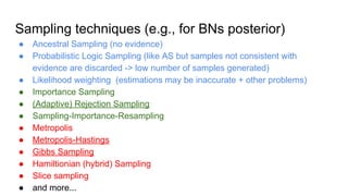


![JAGS PMF-like example: model file
model{#########START###########
sv ~ dunif(0,100)
su ~ dunif(0,100)
s ~ dunif(0,100)
tau <- 1/(s*s)
tauv <- 1/(sv*sv)
tauu <- 1/(su*su)
...
...
for (j in 1:M) {
for (d in 1:D) {
v[j,d] ~ dnorm(0, tauv)
}
}
for (i in 1:N) {
for (d in 1:D) {
u[i,d] ~ dnorm(0, tauu)
}
}
for (j in 1:M) {
for (i in 1:N) {
mu[i,j] <- inprod(u[i,], v[j,])
r3[i,j] <- 1/(1+exp(-mu[i,j]))
r[i,j] ~ dnorm(r3[i,j], tau)
}
}
}#############END############](https://image.slidesharecdn.com/seminar2016-01-20-160210192158/85/Sampling-and-Markov-Chain-Monte-Carlo-Techniques-50-320.jpg)
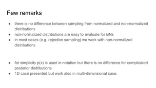
![JAGS PMF-like example: Parameters preparation
n.chains = 1
n.iter = 5000
n.burnin = n.iter
n.thin = 1 #max(1, floor((n.iter - n.burnin)/1000))
D = 10
lu = 0.05
lv = 0.05
n.cluster=n.chains
model.file = "models/pmf_hypnorm3.bug"
N = dim(train)[1]
M = dim(train)[2]
start.s = sd(train[!is.na(train)])
start.su = sqrt(start.s^2/lu)
start.sv = sqrt(start.s^2/lv)
jags.data = list(N=N, M=M, D=D, r=train)
jags.params = c("u", "v", "s", "su", "sv")
jags.inits = list(s=start.s, su=start.su, sv=start.sv,
u=matrix( rnorm(N*D,mean=0,sd=start.su), N, D),
v=matrix( rnorm(M*D,mean=0,sd=start.sv), M, D))](https://image.slidesharecdn.com/seminar2016-01-20-160210192158/85/Sampling-and-Markov-Chain-Monte-Carlo-Techniques-51-320.jpg)

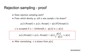
![JAGS PMF-like example: retrieving samples
per.chain = dim(samples$u)[3]
iterations = per.chain * dim(samples$u)[4]
user_sample = function(i, k) {samples$u[i, , (k-1)%%per.chain+1, ceiling(k/per.chain)]}
item_sample = function(j, k) {samples$v[j, , (k-1)%%per.chain+1, ceiling(k/per.chain)]}](https://image.slidesharecdn.com/seminar2016-01-20-160210192158/85/Sampling-and-Markov-Chain-Monte-Carlo-Techniques-53-320.jpg)


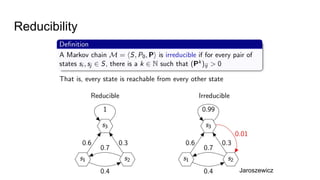
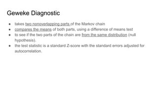
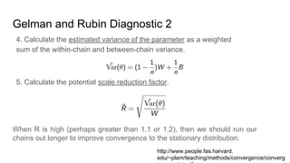
- The document discusses various techniques for Markov chain Monte Carlo (MCMC) sampling, including rejection sampling, Metropolis-Hastings, and Gibbs sampling. - It explains how MCMC can be used for approximate probabilistic inference in complex models by constructing a Markov chain that converges to the target distribution. - Diagnostics are discussed for checking if the Markov chain has converged, such as visual inspection of trace plots, and Geweke and Gelman-Rubin tests of the within-chain and between-chain variances.