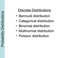
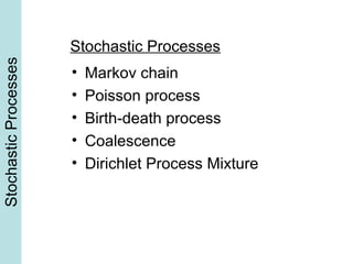
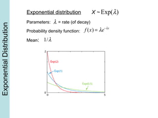
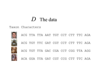
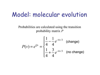
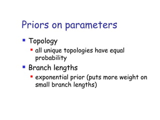
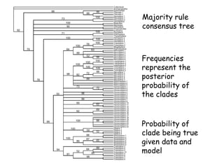
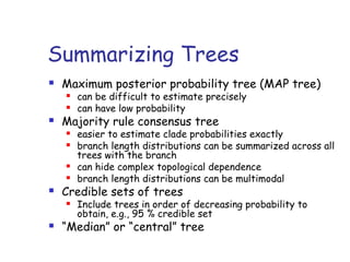
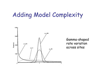
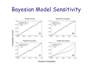
This document provides a summary of Bayesian phylogenetic inference and Markov chain Monte Carlo (MCMC) methods. It begins with an introduction to probability distributions and stochastic processes relevant to phylogenetic modeling. It then discusses how Bayesian inference is applied to phylogenetics by combining prior distributions on tree topologies and other model parameters with the likelihood of the data to obtain posterior distributions. MCMC methods like the Metropolis-Hastings algorithm are introduced as a way to sample from these posterior distributions. Issues around convergence, mixing, and tuning MCMC proposals are also covered.


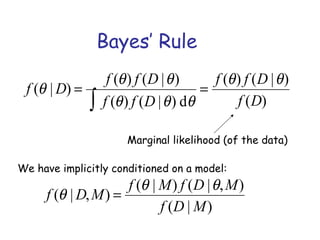
![Model: molecular evolution
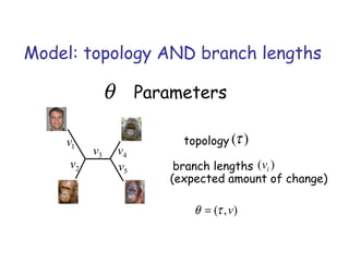
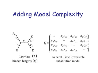
θ Parameters
instantaneous rate matrix
(Jukes-Cantor)
Q =
[A] [C] [G] [T]
[A] − µ µ µ
[C] µ − µ µ
[G] µ µ − µ
[T] µ µ µ −
÷
÷
÷
÷
÷÷](https://image.slidesharecdn.com/bayesianphylogeneticinferencebig4ws2016-10-10-161010141654/85/Bayesian-phylogenetic-inference_big4_ws_2016-10-10-34-320.jpg)


![谷歌留痕技术 [ 𝙩𝙤𝙥 𝟮𝟯𝟯. 𝙘 𝙤𝙢 ]](https://cdn.slidesharecdn.com/ss_thumbnails/top233-260130174328-3833018c-thumbnail.jpg?width=640&height=640&fit=bounds)


