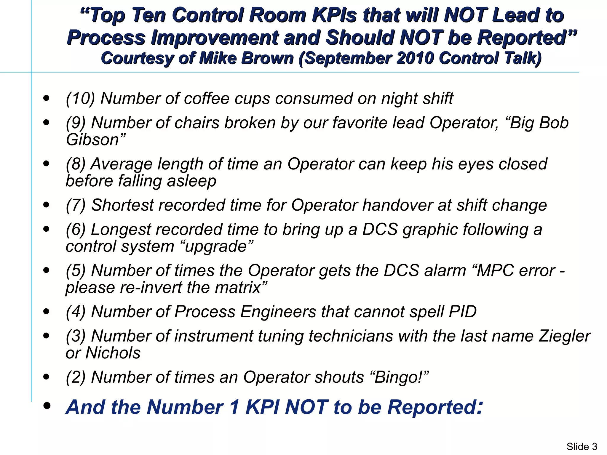
The document outlines a seminar series on PID control of runaway processes, emphasizing the importance of precise temperature control to prevent safety hazards and production issues in various chemical processes. It discusses the tuning of controllers for exothermic reactors, biological reactors, and acid-base systems, highlighting modifications needed for effective management of runaway responses. The document also includes examples of unwanted KPIs to avoid in control room reporting and outlines methods for tuning PID controllers in complex dynamic environments.

1. Interactive Opportunity Assessment Demo and Seminar (Deminar) Series for Web Labs – PID Control of Runaway Processes Aug 25, 2010 Sponsored by Emerson, Experitec, and Mynah Created by Greg McMillan and Jack Ahlers www.processcontrollab.com Website - Charlie Schliesser (csdesignco.com)

2. Welcome Gregory K. McMillan Greg is a retired Senior Fellow from Solutia/Monsanto and an ISA Fellow. Presently, Greg contracts as a consultant in DeltaV R&D via CDI Process & Industrial. Greg received the ISA “Kermit Fischer Environmental” Award for pH control in 1991, the Control Magazine “Engineer of the Year” Award for the Process Industry in 1994, was inducted into the Control “Process Automation Hall of Fame” in 2001, was honored by InTech Magazine in 2003 as one of the most influential innovators in automation, and received the ISA “Life Achievement Award” in 2010. Greg is the author of numerous books on process control, his most recent being Essentials of Modern Measurements and Final Elements for the Process Industry. Greg has been the monthly “Control Talk” columnist for Control magazine since 2002. Greg’s expertise is available on the web site: http://www.modelingandcontrol.com/

3. “ Top Ten Control Room KPIs that will NOT Lead to Process Improvement and Should NOT be Reported” Courtesy of Mike Brown (September 2010 Control Talk) (10) Number of coffee cups consumed on night shift (9) Number of chairs broken by our favorite lead Operator, “Big Bob Gibson” (8) Average length of time an Operator can keep his eyes closed before falling asleep (7) Shortest recorded time for Operator handover at shift change (6) Longest recorded time to bring up a DCS graphic following a control system “upgrade” (5) Number of times the Operator gets the DCS alarm “MPC error - please re-invert the matrix” (4) Number of Process Engineers that cannot spell PID (3) Number of instrument tuning technicians with the last name Ziegler or Nichols (2) Number of times an Operator shouts “Bingo!” And the Number 1 KPI NOT to be Reported :

4. “ Top Ten Control Room KPIs that will NOT Lead to Process Improvement and Should NOT be Reported” Courtesy of Mike Brown (September 2010 Control Talk) (1) Any KPI that needs to be charted with a control range of -1000% to 1000%

5. Introduction Most important and difficult examples are highly exothermic reactors used to produce polymers and specialty chemicals Reaction rate exponentially increases with temperature Tight temperature control is important for batch cycle time, production rate, and product quality (reaction rate maximization and off-spec production minimization depend on operating at maximum temperature that does not trigger side reactions) Tight temperature control is important for safety (a point of return can be reached where reaction heat release rate is greater than heat removal rate causing a high temperature or high pressure trip) Temperature control is extremely sensitive to thermal lags in heat transfer surfaces and in thermowells Open loop tests are deceptive and potentially a safety issue since response looks like an integrator until acceleration kicks-in Controller tuning settings required are unusual. Convention tuning rules can cause slow oscillations, overshoot, and potentially a trip of the safety instrument system (SIS).

6. Introduction Biological reactors in the exponential growth phase can have a runaway response for cell concentration control but the time constant is so slow it often does not present a control problem Strong acid and base pH control systems can exhibit a near runaway response for excursions toward the neutral point due to extreme nonlinearity (orders of magnitude increase in titration curve slope in approach to 7 pH causes acceleration) An axial compressor speed control system can exhibit a severe extremely fast runaway response during surge due to unloading A speed derivative unit that tripped the compressor on high acceleration prevented rotor damage from excessive vibration (benefits: $1,000K/yr savings in eliminating damaged rotors and need to stock multiple rotors)

7. Demos of Exothermic Reactor Acceleration at high temperatures Dynamics and tuning for clean heat transfer surface Modified short cut open loop tuning method Modified ultimate oscillation closed loop tuning method Dynamics and tuning for fouled heat transfer surface Modified ultimate oscillation closed loop tuning method Window of allowable controller gains Major decrease in controller gain

8. Unstable Scenarios

9. Runaway Response For safety reasons, tests are terminated after 4 deadtimes Response to change in controller output with controller in manual  p  p ’ Noise Band Acceleration  CV  CO  CV K p =  CV  CO Runaway process gain (%/%) % Controlled Variable (CV) or % Controller Output (CO) Time (seconds) observed process deadtime runaway process positive feedback time constant

10. Runaway Tuning Modifications for Near Integrator Method (Deminar #6) Increase gain by 25% Increase reset time by factor of 10 Double rate time

11. Acceleration at High Temperatures Objective – Show how runway response initially looks like an integrating but then accelerates Activities: For Single Runaway Loop: Set AC1-1 reset time = 1000 sec Set primary process gain = 2.2 Set AC1-1 manual output = 25% and setpoint = 55% Momentarily set primary process Lag 2 to 1 sec to line out process at setpoint Set primary process deadtime = 8 sec Set primary process Lag 2 = 100 sec Set primary process type = Runaway Change in AC1-1 output from 25% to 35% Measure the deadtime and initial rate of change Note acceleration Stabilize process at 55% setpoint by momentarily switching back to self-regulating process with 1 sec primary process time constant and manual output of 25% Put AC1-1 in auto

12. Tuning for Today’s Example Using Short Cut Near Integrator Method Fastest initial ramp rate estimated in 2 deadtime interval For safety reasons do not keep loop in manual for more than 4 deadtimes! Process Dynamics in Single Loop Lab Near Integrator PID Tuning Modified for Runaway Processes Derivative action must be used to compensate for secondary lags and help prevent acceleration !

13. Short Cut Tuning for Clean Heat Transfer Surface Objective – Show performance of modified short cut method for runaway and start ultimate oscillation Activities: For Single Runaway Loop: Set AC1-1 gain = 2.8, reset = 400 sec, and rate = 4 Make setpoint change from 55% to 60% To create ultimate oscillations set reset time = 10,000, rate = 0, and gain = 7

14. Phase Shift (  ) and Amplitude Ratio (B/A) A B time phase shift  oscillation period T o If the phase shift is -180 o between the process input A and output B , then the total shift for a control loop is -360 o and the output is in phase with the input (resonance) since there is a -180 o from negative feedback (control error = set point – process variable). This point sets the ultimate gain and period that is important for controller tuning.

15. Basis of First Order Approximation  =  Tan -1 (  ) negative phase shift (as  approaches infinity,  approaches -90 o phase shift)  t = (-360  T o time shift B 1 AR = ---- = ----------------------- amplitude ratio A [1 + (   ] 1/2 Amplitude ratios are multiplicative (AR = AR 1  AR 2 ) and phase shifts are additive (     )  asis of first order approx method where gains are multiplicative and dead times are additive

16. Time (min) Process Variable Ultimate Gain is Controller Gain that Caused these Nearly Equal Amplitude Oscillations (K u ) Ultimate Period T u 0 1 K u = ---------------- K p * AR - 180 Ultimate gain of controller is inversely proportional to the product of the open loop static (process) gain and the amplitude ratio at -180 o phase shift, which is the starting point of resonance and instability (growing oscillations) 2  T u = --------  n Ultimate period of control loop occurs at natural frequency  n (at -180 phase shift) Ultimate Gain and Period

17. Runaway Ultimate Gain Calculation  [1 + (  1  u      [1 + (  p ’  T u   ] 1/2 K u = ------------------------------------------------------------------- K p For T u < <   (loop dominated by a large time constant), the error is negligible for the following simplification: (      p ’ K u = ------------------------ K p  T u 2

18. Integrating Process Data Fit from Nyquist Plots: (for  o   simplifies to Near-Integrating process T u )    0.65 T u = 4    1 +    o  o Runaway Process Data Fit from Nyquist Plots : (for  p ’   and  p ’   simplifies to Integrating process T u ) N 0.65 N = (  p ’   )  p ’   T u = 4    1 +    o D D = (  p ’   )  (  p ’  o )  o As either    or  o approach   ’ , D approaches zero, T u approaches infinity, and the controller is unstable for all tuning settings (window of allowable gains is closed) Equations to Estimate Ultimate Period Source: Tuning and Control Loop Performance - My First Book and Creative Work (1984) Self-Regulating Process Data Fit from Bode Plots: (for near-integrating process T u  o )  1  0.65 T u = 2    1 +    o  p  o

19. For a Proportional plus Integral plus Derivative (PID) controller: K c = 0.4  K u 0.5*1.25 x Ziegler-Nichols (0.64) controller gain factor T i = 10  T u 20 x Ziegler-Nichols (0.5) integral time factor T d = 0.125  T u Ziegler-Nichols (0.125) integral time factor Ultimate Oscillation Tuning Modified for Runaway Process Manual methods pose a safety risk, so damped small rather than large equal amplitude oscillations are used Auto and adaptive tuners are preferred that maintain or use closed loop control The relay method on-demand auto tuner will automatically compute the Ultimate Period and Ultimate Gain Window of Allowable Controller Gains 1/ K p > K c < K u

20. Ultimate Oscillation Tuning for Clean Heat Transfer Surface Objective – Show how Ziegler-Nichols tuning settings are modified for runaway Activities: For Single Runaway Loop: Measure ultimate period and note ultimate gain Compute tuning settings by factoring ultimate period and ultimate gain

21. For a Proportional plus Integral plus Derivative (PID) controller: K c = 0.4  K u  T i = 10  T u  T d = 0.125  T u  Ultimate Oscillation Tuning for Clean Heat Transfer Surface

22. Loop Block Diagram (First Order Approximation)  p1  p2  ‘ p2 K pv  p1  c1  m2  m2  m1  m1 K cv  c  c2 Valve Process Controller Measurement K mv  v  v K L  L  L Load Upset  CV  CO  MV  PV PID Delay Lag Delay Delay Delay Delay Delay Delay Lag Lag Lag Lag Lag Lag Lag Gain Gain Gain Gain Local Set Point  DV First Order Approximation :  o  v  p1  p2  m1  m2  c  v  p1  m1  m2  c1  c2 % % % Delay => Dead Time Lag =>Time Constant K i = K mv  (K pv /  p2 )  K cv 100% / span Positive Feedback Time Lag K c T i T d

23.  CV  change in controlled variable (%)  CO  change in controller output (%) K c  controller gain (dimensionless) K i  integrating gain (%/sec/% or 1/sec) K p  process gain (dimensionless) also known as open loop gain MV  manipulated variable (engineering units) PV  process variable (engineering units)  t  change in time (sec)  o  total loop dead time (sec)  m  measurement time constant (sec)  p  process time constant (sec) also known as open loop time constant T i  integral (reset) time setting (sec/repeat) T d  derivative (rate) time setting (sec) T o  oscillation period (sec)   Lambda (closed loop time constant or arrest time) (sec)  f   Lambda factor (ratio of closed to open loop time constant or arrest time) Nomenclature

24. Dynamics and Tuning for Fouled Heat Transfer Surface Objective – Show increase in ultimate period due to fouling of heat transfer surface Activities: For Single Runaway Loop: Increase secondary process Lag2 from 2 to 20 sec To create ultimate oscillations set reset time = 10,000, rate = 0, and gain = 4

25. For Runaway Process: N 0.65 N = (  p ’   )  p ’   = 120*100*20 = 240,000 T u = 4    1 +    o D D = (  p ’   )  (  p ’  o )  o = 80*90*10 = 72,000 (N/D) 0.65 = (240,000/72,000) 0.65 = 2.2 T u = 4    1 +    115 sec Ultimate Period for Fouled Heat Transfer Surface pure deadtime (secondary lag taken as   )

26. Tuning for Fouled Heat Transfer Surface Objective – See extreme effect of secondary lag on ultimate period of runaway process Activities: For Single Runaway Loop: Measure ultimate period and note ultimate gain

27. For a Proportional plus Integral plus Derivative (PID) controller: K c = 0.4  K u  T i = 10  T u  T d = 0.125  T u  Ultimate Oscillation Tuning for Fouled Heat Transfer Surface

28. Window of Allowable Controller Gains Objective – Show effect of controller gain below low gain limit (process diverges from setpoint and goes off scale) Activities: For Single Runaway Loop: Decrease AC1-1 gain to 0.2

29. Visit http://www.processcontrollab.com/ to Create Valuable New Skills Free State of the Art Virtual Plant Independent Interactive Study Learn in 10 minutes rather than 10 years Online Performance Metrics Standard Operator Graphics & Historian Control Room Type Environment No Modeling Expertise Needed No Configuration Expertise Needed Rapid Risk-Free Plant Experimentation Deeper Understanding of Concepts Process Control Improvement Demos Sample Lessons (Recorded Deminars)

30. Help Us Improve These Deminars! WouldYouRecommend.Us/105679s21/

31. Join Us Sept 8, Wednesday 10:00 am CDT Control Loop Performance Primer (The “WHAT” and “WHY” needed to improve 90% of the loops) Look for a recording of Today’s Deminar later this week at: www.ModelingAndControl.com www.EmersonProcessXperts.com

32. QUESTIONS?