Downloaded 311 times
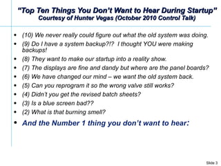


![Integrating Process Open Loop Response Maximum speed in 4 deadtimes is critical speed Time (seconds) o K i = { [ CV 2 t 2 ] CV 1 t 1 ] } CO CO ramp rate is CV 1 t 1 ramp rate is CV 2 t 2 CO CV Integrating process gain (%/sec/%) Response to change in controller output with controller in manual % Controlled Variable (CV) or % Controller Output (CO) observed total loop deadtime](https://image.slidesharecdn.com/process-control-improvement-primer-greg-mcmillan-deminar-100908081456-phpapp01/85/Process-Control-Improvement-Primer-Greg-McMillan-Deminar-19-320.jpg)


This document provides a summary of a seminar on process control improvement concepts. It discusses key concepts like delay, speed, gain, sensitivity, nonlinearity, noise and oscillations. It explains how minimizing delays, maximizing speeds and gains, and reducing nonlinearities can improve control loop performance. Examples of sources of each concept are given for processes, measurements, controllers and final control elements. Graphs are included to show open loop responses for different process types.