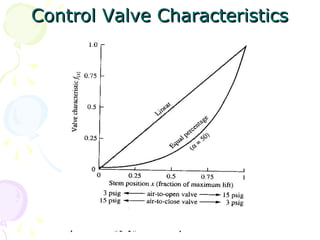
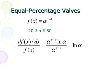
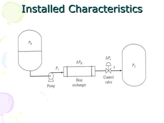
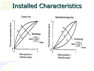
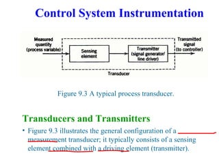
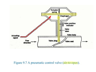
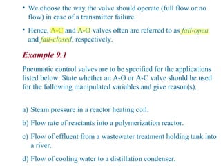
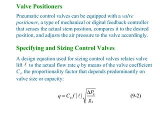
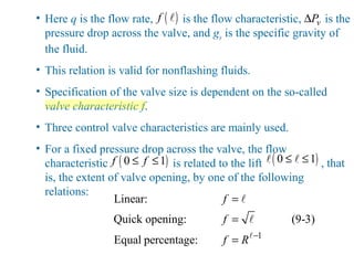
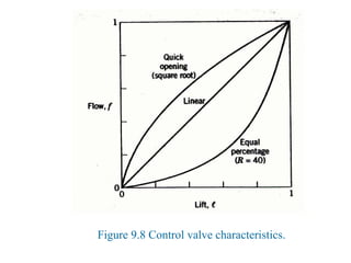
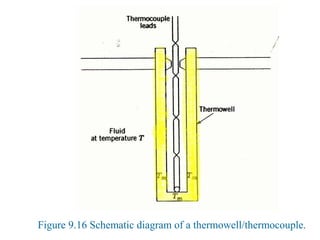
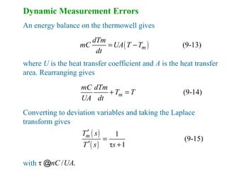
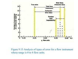
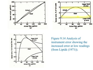
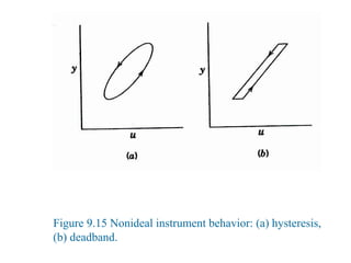
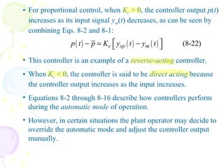
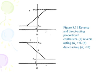
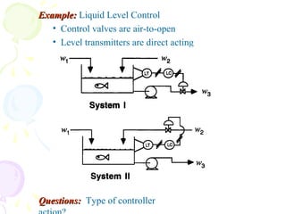
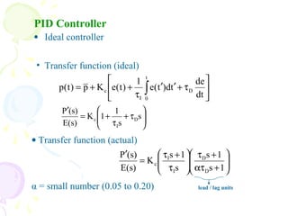
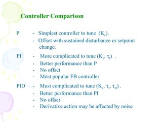
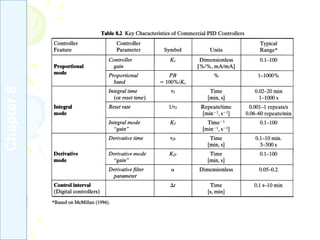
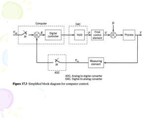
This document discusses instrumentation and control systems. It provides information on common devices used to measure process variables like pressure, temperature, and flow rate. These include transducers, sensors, and transmitters. It also discusses final control elements like control valves and how they are used to manipulate process variables. The document explains the characteristics of different types of control valves and how their flow properties are defined by equations. It also covers topics like pneumatic control systems, calibration of instruments, and algorithms for digital PID control.

1. CONTROLCONTROL
SYSTEMSYSTEM
INSTRUMENTATIONINSTRUMENTATION

5. Control System Instrumentation
Figure 9.3 A typical process transducer.
Transducers and Transmitters
• Figure 9.3 illustrates the general configuration of a
measurement transducer; it typically consists of a sensing
element combined with a driving element (transmitter).

6. • Transducers for process measurements convert the magnitude of
a process variable (e.g., flow rate, pressure, temperature, level,
or concentration) into a signal that can be sent directly to the
controller.
• The sensing element is required to convert the measured
quantity, that is, the process variable, into some quantity more
appropriate for mechanical or electrical processing within the
transducer.
Standard Instrumentation Signal Levels
• Before 1960, instrumentation in the process industries utilized
pneumatic (air pressure) signals to transmit measurement and
control information almost exclusively.
• These devices make use of mechanical force-balance elements
to generate signals in the range of 3 to 15 psig, an industry
standard.

7. • Since about 1960, electronic instrumentation has come into
widespread use.
Sensors
The book briefly discusses commonly used sensors for the most
important process variables. (See text.)
Transmitters
• A transmitter usually converts the sensor output to a signal level
appropriate for input to a controller, such as 4 to 20 mA.
• Transmitters are generally designed to be direct acting.
• In addition, most commercial transmitters have an adjustable
input range (or span).
• For example, a temperature transmitter might be adjusted so that
the input range of a platinum resistance element (the sensor) is
50 to 150 °C.

8. Chapter9

9. • In this case, the following correspondence is obtained:
Input Output
50 °C 4 mA
150 °C 20 mA
• This instrument (transducer) has a lower limit or zero of 50 °C
and a range or span of 100 °C.
• For the temperature transmitter discussed above, the relation
between transducer output and input is
( ) ( )
( )
20 mA 4 mA
mA 50 C 4 mA
150 C 50 C
mA
0.16 C 4 mA
C
mT T
T
 −
= − + ÷
− 
 
= − ÷
 
o
o o
o
o

10. The gain of the measurement element Km is 0.16 mA/°C. For any
linear instrument:
range of instrument output
(9-1)
range of instrument input
mK =
Final Control Elements
• Every process control loop contains a final control element
(actuator), the device that enables a process variable to be
manipulated.
• For most chemical and petroleum processes, the final control
elements (usually control valves) adjust the flow rates of
materials, and indirectly, the rates of energy transfer to and
from the process.

11. Figure 9.4 A linear instrument calibration showing its zero
and span.

12. Control Valves
• There are many different ways to manipulate the flows of
material and energy into and out of a process; for example, the
speed of a pump drive, screw conveyer, or blower can be
adjusted.
• However, a simple and widely used method of accomplishing
this result with fluids is to use a control valve, also called an
automatic control valve.
• The control valve components include the valve body, trim,
seat, and actuator.
Air-to-Open vs. Air-to-Close Control Valves
• Normally, the choice of A-O or A-C valve is based on safety
considerations.

13. Figure 9.7 A pneumatic control valve (air-to-open).

14. • We choose the way the valve should operate (full flow or no
flow) in case of a transmitter failure.
• Hence, A-C and A-O valves often are referred to as fail-open
and fail-closed, respectively.
Example 9.1
Pneumatic control valves are to be specified for the applications
listed below. State whether an A-O or A-C valve should be used
for the following manipulated variables and give reason(s).
a) Steam pressure in a reactor heating coil.
b) Flow rate of reactants into a polymerization reactor.
c) Flow of effluent from a wastewater treatment holding tank into
a river.
d) Flow of cooling water to a distillation condenser.

15. Valve Positioners
Pneumatic control valves can be equipped with a valve
positioner, a type of mechanical or digital feedback controller
that senses the actual stem position, compares it to the desired
position, and adjusts the air pressure to the valve accordingly.
Specifying and Sizing Control Valves
A design equation used for sizing control valves relates valve
lift to the actual flow rate q by means of the valve coefficient
Cv, the proportionality factor that depends predominantly on
valve size or capacity:
l
( ) (9-2)v
v
s
P
q C f
g
∆
= l

16. • Here q is the flow rate, is the flow characteristic, is the
pressure drop across the valve, and gs is the specific gravity of
the fluid.
• This relation is valid for nonflashing fluids.
• Specification of the valve size is dependent on the so-called
valve characteristic f.
• Three control valve characteristics are mainly used.
• For a fixed pressure drop across the valve, the flow
characteristic is related to the lift , that
is, the extent of valve opening, by one of the following
relations:
( )f l vP∆
( )0 1f f≤ ≤ ( )0 1≤ ≤l l
1
Linear:
Quick opening: (9-3)
Equal percentage:
f
f
f R −
=
=
= l
l
l

17. Figure 9.8 Control valve characteristics.

18. Figure 9.16 Schematic diagram of a thermowell/thermocouple.

19. Dynamic Measurement Errors
An energy balance on the thermowell gives
( ) (9-13)m
dTm
mC UA T T
dt
= −
where U is the heat transfer coefficient and A is the heat transfer
area. Rearranging gives
(9-14)m
mC dTm
T T
UA dt
+ =
Converting to deviation variables and taking the Laplace
transform gives
( )
( )
1
(9-15)
τ 1
mT s
T s s
′
=
′ +
with τ / .mC UA@

20. Figure 9.13 Analysis of types of error for a flow instrument
whose range is 0 to 4 flow units.

21. Figure 9.14 Analysis of
instrument error showing the
increased error at low readings
(from Lipták (1971)).

22. Figure 9.15 Nonideal instrument behavior: (a) hysteresis,
(b) deadband.

23. • Example:Example: Flow Control Loop
Assume FT is direct-acting.
1. Air-to-open (fail close) valve ==> ?
2. Air-to-close (fail open) valve ==> ?

24. Automatic and Manual Control Modes
• Automatic Mode
Controller output, p(t), depends on e(t), controller
constants, and type of controller used.
( PI vs. PID etc.)
• Manual Mode
Controller output, p(t), is adjusted manually.
• Manual Mode is very useful when unusual
conditions exist:
plant start-up
plant shut-down
emergencies
• Percentage of controllers "on manual” ??
(30% in 2001, Honeywell survey)

25. • For proportional control, when Kc > 0, the controller output p(t)
increases as its input signal ym(t) decreases, as can be seen by
combining Eqs. 8-2 and 8-1:
( ) ( ) ( ) (8-22)c sp mp t p K y t y t − = − 
• This controller is an example of a reverse-acting controller.
• When Kc < 0, the controller is said to be direct acting because
the controller output increases as the input increases.
• Equations 8-2 through 8-16 describe how controllers perform
during the automatic mode of operation.
• However, in certain situations the plant operator may decide to
override the automatic mode and adjust the controller output
manually.

26. Figure 8.11 Reverse
and direct-acting
proportional
controllers. (a) reverse
acting (Kc > 0. (b)
direct acting (Kc < 0)

27. Example:Example: Liquid Level Control
• Control valves are air-to-open
• Level transmitters are direct acting
Questions:Questions: Type of controller

28. PID Controller
• Ideal controller






τ+′′
τ
++= ∫
t
0
D
I
c
dt
de
td)t(e
1
)t(eKp)t(p






τ+
τ
+=
′
s
s
1
1K
E(s)
(s)P
D
I
c
• Transfer function (ideal)
• Transfer function (actual)
α = small number (0.05 to 0.20)






+ατ
+τ






τ
+τ
=
′
1s
1s
s
1s
K
E(s)
(s)P
D
D
I
I
c
lead / lag units

29. PID - Most complicated to tune (Kc, τI, τD) .
- Better performance than PI
- No offset
- Derivative action may be affected by noise
PI - More complicated to tune (Kc, τI) .
- Better performance than P
- No offset
- Most popular FB controller
P - Simplest controller to tune (Kc).
- Offset with sustained disturbance or setpoint
change.
Controller Comparison

30. Typical Response of Feedback Control Systems
Consider response of a controlled system after a
sustained disturbance occurs (e.g., step change in
the disturbance variable)
Figure 8.12. Typical process responses with feedback control.

31. Figure 8.13.
Proportional control:
effect of controller
gain.
Figure 8.15. PID
control: effect of
derivative time.

32. Figure 8.14. PI control: (a) effect of reset time (b) effect of
controller gain.

33. Chapter8

37. Position and Velocity Algorithms for Digital PID
Control
A straightforward way of deriving a digital version of the parallel
form of the PID controller (Eq. 8-13) is to replace the integral and
derivative terms by finite difference approximations,
( )0
1
* (8-24)
kt
j
j
e t dt e t
=
≈ ∆∑∫
1
(8-25)k ke ede
dt t
−−
≈
∆
where:
= the sampling period (the time between successive
measurements of the controlled variable)
ek = error at the kth sampling instant for k = 1, 2, …
t∆

38. There are two alternative forms of the digital PID control
equation, the position form and the velocity form. Substituting (8-
24) and (8-25) into (8-13), gives the position form,
( )1
1 1
(8-26)
k
D
k c k j k k
j
t
p p K e e e e
t
τ
τ
−
=
 ∆
= + + + − 
∆  
∑
Where pk is the controller output at the kth sampling instant. The
other symbols in Eq. 8-26 have the same meaning as in Eq. 8-13.
Equation 8-26 is referred to as the position form of the PID
control algorithm because the actual value of the controller output
is calculated.

39. (8-27)
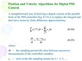
Note that the summation still begins at j = 1 because it is assumed
that the process is at the desired steady state for
and thus ej = 0 for . Subtracting (8-27) from (8-26)
gives the velocity form of the digital PID algorithm:
In the velocity form, the change in controller output is
calculated. The velocity form can be derived by writing the
position form of (8-26) for the (k-1) sampling instant:
0j ≤ 0j ≤
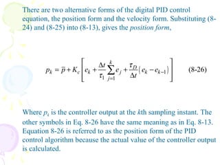
( ) ( )1 1 1 22
(8-28)
D
k k k c k k k k k k
I
t
p p p K e e e e e e
t
τ
τ− − − −
 ∆
∆ = − = − + + − + 
∆ 
[ ])( 21
1
1
11 −−
−
=
−− −
∆
+
∆
++= ∑ kk
D
k
j
j
I
kck ee
t
e
t
eKpp
τ
τ

40. [ ])( 21
1
1
11 −−
−
=
−− −
∆
+
∆
++= ∑ kk
D
k
j
j
I
kck ee
t
e
t
eKpp
τ
τ
( )1
1 1
(8-26)
k
D
k c k j k k
j
t
p p K e e e e
t
τ
τ
−
=
 ∆
= + + + − 
∆  
∑
( ) ( )1 1 1 22
(8-28)
D
k k k c k k k k k k
I
t
p p p K e e e e e e
t
τ
τ− − − −
 ∆
∆ = − = − + + − + 
∆ 
(8-27)

41. The velocity form has three advantages over the position form:
1. It inherently contains anti-reset windup because the
summation of errors is not explicitly calculated.
2. This output is expressed in a form, , that can be utilized
directly by some final control elements, such as a control
valve driven by a pulsed stepping motor.
3. For the velocity algorithm, transferring the controller from
manual to automatic mode does not require any initialization
of the output ( in Eq. 8-26). However, the control valve (or
other final control element) should be placed in the
appropriate position prior to the transfer.
kp∆
p

42. TransmittersTransmitters

43. Typical Air-Operated Control ValveTypical Air-Operated Control Valve

44. Control Valve CharacteristicsControl Valve Characteristics
• The valve equation for liquids is
• Linear-trim valves:
• Equal-percentage-trim valves:
..
)(
grsp
P
xfCF V
V
∆
=
xxf =)(
1
)( −
= x
xf α

45. Control Valve CharacteristicsControl Valve Characteristics

46. Equal-Percentage ValvesEqual-Percentage Valves
20 α 50≦ ≦
1
)( −
= x
xf α
α
α
αα
ln
ln
)(
/)(
1
1
== −
−
x
x
xf
dxxdf

47. Installed CharacteristicsInstalled Characteristics

48. Installed CharacteristicsInstalled Characteristics