process control cha 3

1. Lecture Three
Process Control Tuning
Goitom Tadesse (M/Tech)
Defence Engineering College
Process Control Fundamentals
EP-5512
Mar. 2019

2. Introduction
What is the aim of the controller tuning? If it was
possible to obtain, it would be like to obtain both of
the following for the control system:
• Fast responses, and
• Good stability
Unfortunately, for practical systems these two wishes
can not be achieved simultaneously. In other words:
• The faster response, the worse stability, and
• The better stability, the slower response.
2

3. Process Control …
So, for the control system, we look the following
compromise:
Acceptable stability, and medium fastness of response
3

4. Process Control …
Approaches to process control:
1.No Control: Naturally, the easiest approach is to do
nothing other than to hold all input variables close to
their design values.
This approach could have serious effects on safety,
product quality, and profit and is not generally
acceptable for important variables.
2.Manual Operation: When corrective action is taken
periodically by operating personnel, the approach is
usually termed manual (or open-loop) operation.
4

5. This approach is not always bad or "low-technology,"
so we should understand when and why to use it.
3.On-Off Control: The simplest form of automated
control involves logic for the control calculations.
In this approach, trigger values are established, and
the control manipulation changes state when the
trigger value is reached.
While appealing because of its simplicity, on/off
control results in continuous cycling, and
performance is generally unacceptable for the strict
requirements of many processes.
Process Control …
5

6. 4. Continuous Automated Control: This approach offers
the best control performance for most process
situations and can be easily automated using
computing equipment.
5.Emergency Controls: Continuous control performs
well in maintaining the process near its set point.
However, continuous control does not ensure that the
controlled variable remains within acceptable.
The emergency controls measure a key variable(s)
and take extreme action before a violation occurs;
Process Control …
6

7. this action could include stopping all or critical flow
rates or dramatically increasing cooling duty.
The control calculations for emergency control are
usually not complex, but the detailed design of
features such as sensor and valve locations is crucial
to safe plant design and operation.
In industrial plants all five control approaches are
used concurrently.
Plant personnel continuously monitor plant
performance, make periodic changes to achieve
control of some variables.
Process Control …
7

8. Process Control …
Key performance feature of feedback control
algorithm:
The purpose of the feedback control loop is to
maintain a small deviation between the CV and the SP
by adjusting the MV.
Control performance depends on the goals of the
process operation.
Offset: Offset is a difference between final, steady-
state values of the set point and of the controlled
variable.
8

9. Process Control …
In most cases, a zero steady-state offset is highly
desired, because the control system should achieve
the desired value, at least after a very long time.
9

10. Process Control …
Rise Time (Tr): is the time from the step change in
the set point until the controlled variable first reaches
the new set point. A short rise time is usually desired.
Decay Ratio (B/A): The decay ratio is the ratio of
neighboring peaks in an underdamped controlled-
variable response.
Usually, periodic behavior with large amplitudes is
avoided in process variables; therefore, a small decay
ratio is usually desired, and an overdamped response
is sometimes desired.
10

11. Process Control …
Period Of Oscillation (P): depends on the process
dynamics and is an important characteristic of the
closed-loop response.
It is not specified as a control performance goal.
Settling Time: is the time the system takes to attain a
"nearly constant" value, usually ±5 % of its final
value.
This measure is related to the rise time and decay
ratio.
A short settling time is usually favored.
11

12. Process Control …
MV Overshoot (C/D): This quantity is of concern
because the manipulated variable is also a process
variable that influences performance.
There are often reasons to prevent large variations in
the manipulated variable.
Some large manipulations can cause long-term
degradation in equipment performance; an example
is the fuel flow to a furnace or boiler, where frequent,
large manipulations can cause undue thermal stresses.
12

13. Process Control …
On the other hand, some manipulated variables can be
adjusted without concern, such as cooling water flow.
We will use the overshoot of the manipulated variable
as an indication of how aggressively it has been
adjusted.
The overshoot is the maximum amount that the
manipulated variable exceeds its final steady-state
value and is usually expressed as a percent of the
change in manipulated variable from its initial to its
final value.
13

14. Process Control …
Zero Offset: The performance measures could be
combined into two categories:
Dynamic (IAE, ISE, damping ratio, settling time, etc.)
and steady-state.
Integral Error Measures: These indicate the
cumulative deviation of the controlled variable from
its set point during the transient response. Several
such measures are used:
Integral of the absolute value of the error (IAE):
14
0
|SP( ) CV( ) |IAE t t dt

 

15. Process Control …
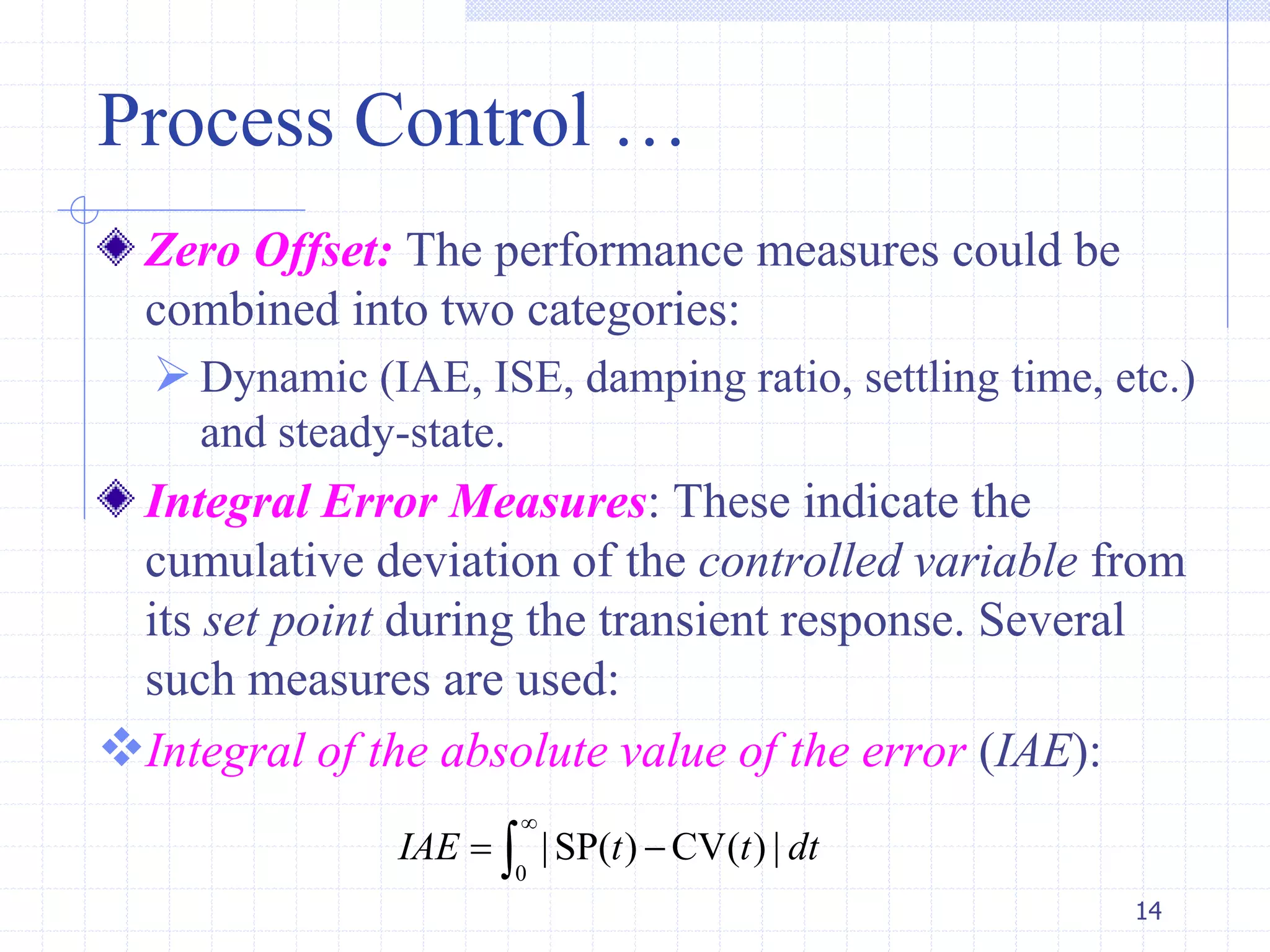
The IAE is an easy value to analyze visually, because
it is the sum of areas above and below the set point.
It is an appropriate measure of control performance
when the effect on control performance is linear with
the deviation magnitude.
Integral of square of the error (ISE):
The ISE is appropriate when large deviations cause
greater performance degradation than small
deviations.
15
2
0
[SP( ) CV( )]ISE t t dt

 

16. Process Control …
Integral of product of time and the absolute value of
error (ITAE):
The ITAE penalizes deviations that endure for a long
time.
Integral of the error (IE):
Note that IE is not used, because positive and
negative errors cancel in the integral, resulting in the
possibility for large positive and negative errors to
give a small IE. A small integral error measure (e.g.,
IAE) is desired. 16
0
|SP( ) CV( ) |ITAE t t t dt

 
0
[SP( ) CV( )]IE t t dt

 

17. Process Control …
The steady-state goal, returning to set point, can be
stated mathematically by using the final value
theorem:
Insensitivity to Errors: we can never model a process
exactly. Because parameters in all control algorithms
depend on process models, control algorithms will
always be in error despite our best modeling efforts.
Therefore, control algorithms should provide good
performance when the adjustable parameters have
"reasonable" errors.
17
0
lim ( ) lim ( ) 0
t s
E t sE s
 
 

18. Process Control …
Naturally, all algorithms will give poor performance
when the adjustable parameter errors are very large.
Wide Applicability: The PID control algorithm is a
simple, single equation, but it can provide good
control performance for many different processes.
This flexibility is achieved through several adjustable
parameters, whose values can be selected to modify
the behavior of the feedback system.
The procedure for selecting the values is termed
tuning, and the adjustable parameters are termed
tuning constants.
18

19. Process Control …
Timely Calculations: The control calculation is part
of the feedback loop, and therefore it should be
calculated rapidly and reliably.
Excessive time for calculation would introduce an
extra slow element in the control loop and, as we
shall see, degrade the control performance.
Iterative calculations, which might occasionally not
converge, would result in a loss of control at
unpredictable times.
19

20. Process Control …
The PID algorithm is exceptionally simple, a feature
that was crucial to its initial use but is not as
important now due to the availability of inexpensive
digital computers for control.
Because of its wide use, the PID controller is
available in nearly all commercial digital control
systems, so that efficiently programmed and well-
tested implementations are available.
20

21. Process Control …
Enhancements: No single algorithm can address all
control requirements.
A convenient feature of the PID algorithm is its
compatibility with enhancements that provide
capabilities not in the basic algorithm.
Thus, we can enhance the basic PID without
discarding it.
PID controllers have been at the heart of control
engineering practice for decades.
21

22. PID Control Tuning
In process control, more than 95% of the control
loops are of the PID type.
A portion of the signal being fed back is:
 Proportional to the signal (P)
 Proportional to integral of the signal (I)
 Proportional to the derivative of the signal (D)
PID control works well on SISO systems, where a
desired Set Point can be supplied to the system
control input
22

23. PID Control …
PID control handles
step changes to the
Set Point especially well:
• Fast Rise Times
• Little or No Overshoot
• Fast settling Times
• Zero Steady State Error
PID controllers are often fine tuned on-site, using
established guidelines
23

24. 24
 Closed-loop transfer functions for a feedback loop
 Disturbance response:
 Set point response:
( )( )
( ) 1 ( ) ( ) ( ) ( )
d
p v c s
G sCV s
D s G s G s G s G s


( ) ( ) ( )( )
( ) 1 ( ) ( ) ( ) ( )
p v c
p v c s
G s G s G sCV s
SP s G s G s G s G s


PID Control …

25. PID Control …
Proportional Control Mode: A corrective force that
is proportional to the amount of error.
MV = KcE + Bias
MV = Controller Output due to proportional control
Kc = proportional constant for the system called gain
E = error
 Where E = Set Point (SP) – Process Variable (PV)
Bias = used to remove the steady state error at a
particular set point
25
( ) ( )
( )
( )
( )
P c P
P
c c
MV t K E t I
MV s
G s K
E s
 
 

26. Proportional Control …
If we have zero error, our proportional term will
contribute zero to the controller output. Without
error, a proportional controller does nothing! Bias is
used to ensure this is true.
Acts in the now - what is my error now?
Proportional control is used for fast responding
processes that do not require offset free operation
(some specific level, pressure, etc.)
Proportional Control Example:
• Control Output moves actuator to reduce error. As the error
becomes less, so does the output until the set point is reached
26

27. Steady-State-Error: Main problem of proportional
control – when error is close to zero, the force
becomes small and is not enough to overcome friction
- stops before set point.
Dead band or dead zone: area on both sides of set
point
 Friction, backlash, flexing parts, poor controller design
Proportional Control …
27
 Bias sometimes used to
prevent this or one could
increase the gain, but this
may cause oscillations

28. Proportional Control …
Example 1: The three-tank mixing process under
control is now analyzed. Recall that the feedback and
disturbance processes are third-order.
The steady-state value for error under proportional
control can be determined by rearranging the above
transfer function, substituting the models for Gp(s) and
Gd(s), and applying the final value theorem to the
system with a step like disturbance, D(s) = ∆D/s.
Recall that the valve transfer function is included in
Gp(s), and the sensor transfer function is assumed to
be unity, implying instantaneous, error-free
measurement.
28

29. Proportional Control …
Given that
29
3
3
( ) 1, ( ) ( ) ,
( 1)
( ) , ( )
( 1)
p
s p v
d
d c c
K
G s G s G s
s
K
G s G s K
s


 

 

( ) ( )
( )
1 ( ) ( ) ( ) ( )
d
p v c s
D s G s
CV s
G s G s G s G s


0 0
1 1 1
1 1 1
( ) | lim ( ) lim
1 1 1
1
1 1 1
d
t
s s
c p
K
D s s s
CV t sCV s s
s
K K
s s s
  
  

 
    
             
               
0
1
d
c p
K D
K K

 


30. Proportional Control …
Note that the feedback control system with
proportional control does not achieve zero steady-
state offset!
Thus, steady-state offset occurs with proportional-
only control.
This is a serious shortcoming,
which must be corrected by one
of the remaining two modes.
30

31. Integral Control Mode
Integral control is used to reduce steady-state error
to zero.
MV = KI (Et)
MV = Controller Output due to integral control
KI = Kc /TI = integral gain constant
(Et) = sum of all past errors (multiplied by the
time they existed)
31
0
( ) ( )
( )
( )
( )
t
I I I
cI
c
I
MV t K E t dt I
KMV s
G s
E s T s
 
 


32. Integral Control …
The new adjustable parameter is the integral time, TI.
Acts in the past - what was my error?
Sums the error over all past time and multiplies this
summed error value with the tuning parameter.
Creates a restoring force that is proportional to the
sum of all past errors multiplied by time.
For a constant value of error, the value of (Et) will
increase with time causing the restoring force to get
larger and larger.
32

33. Integral Control …
 Eventually, the restoring force will get large enough
to overcome friction and move the controlled variable
in a direction to eliminate the error.
 Integral can be used alone (Very Sluggish), but is
normally used with proportional control for better
responsiveness.
 Example: Integral response can easily be observed on
industrial robots. When a weight is placed on the arm,
it will visibly sag and then restore itself to the original
position.
33

34. Integral Control …
Its problems
• Reduced stability
• Oscillations
• Slow: It takes time for error*time to accumulate.
34

35. Integral Control …
Example 2: The effect of the integral mode can be
determined by evaluating the offset of the three-tank
mixing process under integral-only control for a step
disturbance, D(s) = ∆D/s.
35
3 3
( ) 1, ( ) ( ) , ( ) , ( )
( 1) ( 1)
p d c
s p v d c
I
K K K
G s G s G s G s G s
s s T s 
   
 
0 0
1 1 1
1 1 1
( ) | lim ( ) lim
1 1 1 1
1
1 1 1
0
d
t
s s
c p
I
K
D s s s
CV t sCV s s
s
K K
T s s s s
  
  

 
    
             
      
      
        


36. Integral Control …
The integral control mode achieves zero steady-state
offset, which is the primary reason for including this
mode.
36
• If the integral time is
reduced small enough, the
controller will be very
aggressive, and the system
will become highly
oscillatory; further
reduction in TI can lead to
an unstable system

37. Derivative Control Mode
Derivative control is a solution to the overshoot
problem.
MV = KD (PV / t)
MV = Controller Output due to derivative control
KD = KcTd = derivative gain constant
PV/t = error rate of change (slope of error curve)
PV = Process Variable (sensor reading)
37
( )
( )
( )
( )
( )
d c d d
d
c c d
dE t
MV t K T I
dt
MV s
G s K T s
E s
 
 

38. Derivative Control …
The adjustable parameter is the derivative time Td,
Slows down the controlled variable to minimize
overshoot.
Derivative control is Proportional to error slope.
Helps systems respond quicker to changes in the load
Derivative works by trying to anticipate the future.
Derivative action is never used by itself. It is always
used with P or PI.
Derivative will allow us to use higher controller gains
or can further smooth out integral instability.
38

39. Derivative Control …
39
 Improves system in two ways:
• Extra force to start.
• Provides brakes to slow down
when close to set point.
 Too much derivative control
can cause slow system
response.
 Can cause valve chatter!
 Never used by itself

40. Derivative Control …
Example 3: The offset of a derivative controller can
be determined by applying the final value theorem to
the three-tank mixing process for a step disturbance,
D(s) = ∆D/s.
40
3 3
( ) 1, ( ) ( ) , ( ) , ( )
( 1) ( 1)
p d
s p v d c c d
K K
G s G s G s G s G s K T s
s s 
   
 
0
1 1 1
1 1 1
( ) | lim
1 1 1
1
1 1 1
0
d
t
s
c d p
d
K
D s s s
CV t s
s
K T sK
s s s
K D
  
  


    
            
               
  

41. Proportional-Integral Control
Creates a restoring force that is proportional to the
sum of all past errors multiplied by time.
Where as proportional control works in the present,
integral action works in the past.
PI control is used for fast responding processes that
require offset free operation.
MV = Kc [E + 1/TI (Et)]
41
0
1
( ) ( ) ( )
( ) 1
( ) 1
( )
t
c
I
c c
I
MV t K E t E t dt I
T
MV s
G s K
E s T s
 
   
 
 
   
 


42. Proportional-Derivative Control
PD control is preferred when integral action is not
needed, but the dynamics of the process are so slow
that the predictive nature of the derivative action is
useful.
Many thermal processes, where energy is stored with
small heat losses, usually have small dynamics.
PD controller might be suited for temperature control.
42
 
( )
( ) ( )
( )
( ) 1
( )
c d
c c d
dE t
MV t K E t T I
dt
MV s
G s K T s
E s
 
   
 
  

43. PID Control …
Applies the brakes, slowing the controlled variable
just before it reaches its destination.
If proportional works in the present, and integral
works in the past, derivative works by trying to
anticipate the future.
43
0
1 ( )
( ) ( ) ( )
( ) 1
( ) 1
( )
t
c d
I
c c d
I
dE t
MV t K E t E t dt T I
T dt
MV s
G s K T s
E s T s
 
    
 
 
    
 


44. PID Control …
44
Series or Classical PID– was
the first type of PID control.
It is a nightmare to tune by
trial and error as the terms
affect each other. A change
in P affects the I and D and
so on…

45. PID Control …
45
Parallel: All three
are independent –
results are added at
the end
Ideal or ISA: Not
too bad to tune –
most controllers
today use this method
of control

46. PID Control …
Constants Rise time Overshoot Settling Time ess
Kc ↑ Decrease Increase Small change Decrease
KI ↑ Decrease Increase Increase Eliminate
Kd ↑ Small Change Decrease Decrease Small Change
46
Summary of PID controller

47. The complete circuit for PID controller
PID Control …
47

48. 48