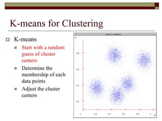
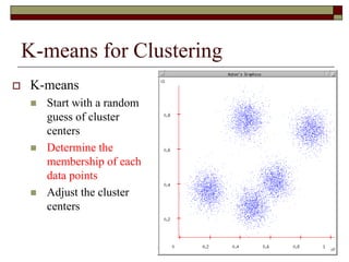
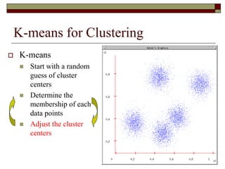
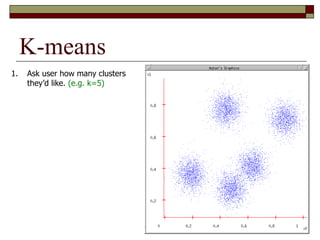
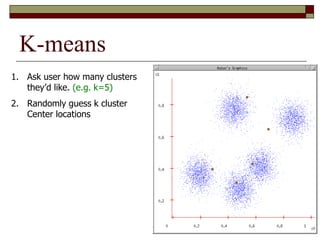
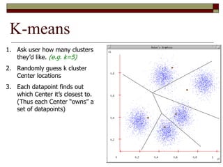
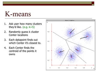
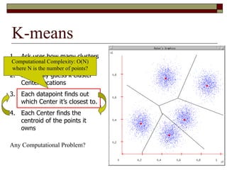
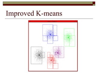
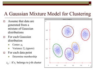
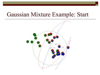
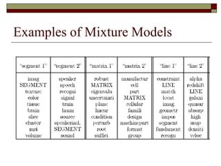
This document provides an overview of clustering techniques including k-means clustering, expectation maximization algorithms, and spectral clustering. It discusses how k-means clustering works by initializing random cluster centers, assigning data points to the closest centers, and adjusting the centers iteratively. Expectation maximization is presented as a way to learn the parameters of a Gaussian mixture model to cluster data. Finally, applications of clustering like document clustering using mixture models are briefly described.

1. Overview of Clustering
Rong Jin

2. Outline
 K means for clustering
 Expectation Maximization algorithm for clustering
 Spectrum clustering (if time is permitted)

3. Clustering
$$$
age
 Find out the underlying structure for given data
points

4. Application (I): Search Result Clustering

5. Application (II): Navigation

6. Application (III): Google News

7. Application (III): Visualization
Islands of music
(Pampalk et al., KDD’ 03)

8. Application (IV): Image Compression
http://www.ece.neu.edu/groups/rpl/kmeans/

9. How to Find good Clustering?
 Minimize the sum of
distance within clusters
C1
C2
C3
C4
C5
 
 
,
6 2
,
1 1,
arg min
j i j
n
i j i j
j iC m
m x C
 
 
,
6
,
1
1 the j-th cluster
0 the j-th cluster
1
any a single cluster
i
i j
i
i j
j
i
x
m
x
m
x


 


 


10. How to Efficiently Clustering Data?
 
 
,
6 2
,
1 1,
arg min
j i j
n
i j i j
j iC m
m x C
 
 
   ,Memberships and centers are correlated.i j jm C
 
,
1
,
,
1
Given memberships ,
n
i j i
i
i j j n
i j
i
m x
m C
m





2
,
1 arg min( )
Given centers { },
0 otherwise
i j
kj i j
j x C
C m
  
 


11. K-means for Clustering
 K-means
 Start with a random
guess of cluster
centers
 Determine the
membership of each
data points
 Adjust the cluster
centers

12. K-means for Clustering
 K-means
 Start with a random
guess of cluster
centers
 Determine the
membership of each
data points
 Adjust the cluster
centers

13. K-means for Clustering
 K-means
 Start with a random
guess of cluster
centers
 Determine the
membership of each
data points
 Adjust the cluster
centers

14. K-means
1. Ask user how many clusters
they’d like. (e.g. k=5)

15. K-means
1. Ask user how many clusters
they’d like. (e.g. k=5)
2. Randomly guess k cluster
Center locations

16. K-means
1. Ask user how many clusters
they’d like. (e.g. k=5)
2. Randomly guess k cluster
Center locations
3. Each datapoint finds out
which Center it’s closest to.
(Thus each Center “owns” a
set of datapoints)

17. K-means
1. Ask user how many clusters
they’d like. (e.g. k=5)
2. Randomly guess k cluster
Center locations
3. Each datapoint finds out
which Center it’s closest to.
4. Each Center finds the
centroid of the points it
owns

18. K-means
1. Ask user how many clusters
they’d like. (e.g. k=5)
2. Randomly guess k cluster
Center locations
3. Each datapoint finds out
which Center it’s closest to.
4. Each Center finds the
centroid of the points it
owns
Any Computational Problem?
Computational Complexity: O(N)
where N is the number of points?

19. Improve K-means
 Group points by region
 KD tree
 SR tree
 Key difference
 Find the closest center for
each rectangle
 Assign all the points within a
rectangle to one cluster

20. Improved K-means
 Find the closest center for
each rectangle
 Assign all the points within
a rectangle to one cluster

21. Improved K-means

22. Improved K-means

23. Improved K-means

24. Improved K-means

25. Improved K-means

26. Improved K-means

27. Improved K-means

28. Improved K-means

29. Improved K-means

30. A Gaussian Mixture Model for Clustering
 Assume that data are
generated from a
mixture of Gaussian
distributions
 For each Gaussian
distribution
 Center: i
 Variance: i (ignore)
 For each data point
 Determine membership
: if belongs to j-th clusterij iz x

31. Learning a Gaussian Mixture
(with known covariance)
 Probability ( )ip x x
 
2
/ 2 2
2
( ) ( , ) ( ) ( | )
1
( ) exp
22
j j
j
i i j j i j
i j
j d
p x x p x x p p x x
x
p
 

     

 

       
 
   
 
 
 


32. Learning a Gaussian Mixture
(with known covariance)
 Probability ( )ip x x
 
2
/ 2 2
2
( ) ( , ) ( ) ( | )
1
( ) exp
22
j j
j
i i j j i j
i j
j d
p x x p x x p p x x
x
p
 

     

 

       
 
   
 
 
 

 Log-likelihood of data
 Apply MLE to find optimal parameters
 
2
/ 2 2
2
1
log ( ) log ( ) exp
22j
i j
i j d
i i
x
p x x p


 

         
   
  
 ( ),j j j
p   

33. Learning a Gaussian Mixture
(with known covariance)
2
2
2
2
1
( )
2
1
( )
2
1
( )
( )
i j
i n
x
j
k x
n
n
e p
e p




 
 
 
 




[ ] ( | )ij j iE z p x x   E-Step
1
( | ) ( )
( | ) ( )
i j j
k
i n j
n
p x x p
p x x p
   
   

  

  

34. Learning a Gaussian Mixture
(with known covariance)
1
1
1
[ ]
[ ]
m
j ij im
i
ij
i
E z x
E z



 

M-Step
1
1
( ) [ ]
m
j ij
i
p E z
m
 

  

35. Gaussian Mixture Example: Start

36. After First Iteration

37. After 2nd Iteration

38. After 3rd Iteration

39. After 4th Iteration

40. After 5th Iteration

41. After 6th Iteration

42. After 20th Iteration

43. Mixture Model for Doc Clustering
 A set of language models

 1 2, ,..., K   
1 2{ ( | ), ( | ),..., ( | )}i i i V ip w p w p w   

44. Mixture Model for Doc Clustering
 A set of language models

 1 2, ,..., K   
1 2{ ( | ), ( | ),..., ( | )}i i i V ip w p w p w   
( )ip d d
( , )
1
( ) ( , )
( ) ( | )
( ) ( | )
j
j
k i
j
i i j
j i j
V tf w d
j k j
k
p d d p d d
p p d d
p p w



 
   
  

   
   
    


 
 Probability

45. Mixture Model for Doc Clustering
 A set of language models

 1 2, ,..., K   
1 2{ ( | ), ( | ),..., ( | )}i i i V ip w p w p w   
( )ip d d
( , )
1
( ) ( , )
( ) ( | )
( ) ( | )
j
j
k i
j
i i j
j i j
V tf w d
j k j
k
p d d p d d
p p d d
p p w



 
   
  

   
   
    


 
 Probability

46. Mixture Model for Doc Clustering
 A set of language models

 1 2, ,..., K   
1 2{ ( | ), ( | ),..., ( | )}i i i V ip w p w p w   
( )ip d d
( , )
1
( ) ( , )
( ) ( | )
( ) ( | )
j
j
k i
j
i i j
j i j
V tf w d
j k j
k
p d d p d d
p p d d
p p w



 
   
  

   
   
    


 
 Probability
Introduce hidden variable zij
zij: document di is generated by the
j-th language model j.

47. Learning a Mixture Model
 
( , )
1
( , )
1 1
( | ) ( )
( | ) ( )
k i
k i
V tf w d
m j j
m
VK
tf w d
m n n
n m
p w p
p w p
  
  

 
   




1
[ ] ( | )
( | ) ( )
( | ) ( )
ij j i
i j j
K
i n n
n
E z p d d
p d d p
p d d p
 
   
   

  
  

  
E-Step
K: number of language models

48. Learning a Mixture Model
M-Step
1
1
( ) [ ]
N
j ij
i
p E z
N
 

  
1
1
[ ] ( , )
( | )
[ ]
N
ij i k
k
i j N
ij k
k
E z tf w d
p w
E z d
 




N: number of documents

49. Examples of Mixture Models

50. Other Mixture Models
 Probabilistic latent semantic index (PLSI)
 Latent Dirichlet Allocation (LDA)

51. Problems (I)
 Both k-means and mixture models need to compute
centers of clusters and explicit distance measurement
 Given strange distance measurement, the center of
clusters can be hard to compute
E.g.,  ' ' '
1 1 2 2' max , ,..., n nx x x x x x x x
    
x y
z
 
  x y x z

52. Problems (II)
 Both k-means and mixture models look for compact
clustering structures
 In some cases, connected clustering structures are more desirable

53. Graph Partition
 MinCut: bipartite graphs with minimal number of
cut edges
CutSize = 2

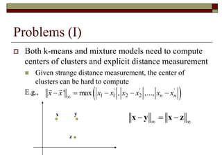
54. 2-way Spectral Graph Partitioning
 Weight matrix W
 wi,j: the weight between two
vertices i and j
 Membership vector q
1 Cluster
-1 Cluster
i
i A
q
i B

 

 
[ 1,1]
2
,
,
arg min
1
4
n
i j i j
i j
CutSize
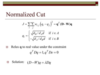
CutSize J q q w
 

  
q
q

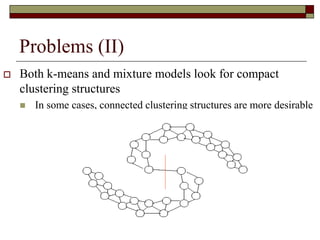
55. Solving the Optimization Problem
 Directly solving the above problem requires
combinatorial search  exponential complexity
 How to reduce the computation complexity?
 
2
,
[ 1,1] ,
1
argmin
4n
i j i j
i j
q q w
 
 
q
q

56. Relaxation Approach
 Key difficulty: qi has to be either –1, 1
 Relax qi to be any real number
 Impose constraint 2
1
n
ii
q n

   
2 2 2
, ,
, ,
2
, ,
,
1 1
2
4 4
1 1
2 2
4 4
i j i j i j i j i j
i j i j
i i j i j i j
i j i j
J q q w q q q q w
q w q q w
    
 
   
 
 
  
,i i j
j
d w 
 2
, , ,
,
1 1 1
2 2 2
i i i j i j i i i j i j j
i i j i
q d q q w q d w q     
,i i jD d    
( )T
J  q D W q

57. Relaxation Approach
2
* argmin argmin ( )
subject to
T
k
k
J
q n
  

q q
q q D W q

58. Relaxation Approach
 Solution: the second minimum eigenvector for D-W
2
* argmin argmin ( )
subject to
T
k
k
J
q n
  

q q
q q D W q
2( )D W  q q

59. Graph Laplacian
 L is semi-positive definitive matrix
 For Any x, we have xTLx  0, why?
 Minimum eigenvalue 1 = 0 (what is the eigenvector?)

 The second minimum eigenvalue 2 gives the best bipartite
graph
 , , ,: ,i j i j i jj
w w         L D W W D
1 2 30 ... k      

60. Recovering Partitions
 Due to the relaxation, q can be any number (not just
–1 and 1)
 How to construct partition based on the eigenvector?
 Simple strategy: { | 0}, { | 0}i iA i q B i q   

61. Spectral Clustering
 Minimum cut does not balance the size of bipartite
graphs

62. Normalized Cut (Shi & Malik, 1997)
 Minimize the similarity between clusters and meanwhile
maximize the similarity within clusters
,( , ) , ,
( , ) ( , )
i j A i B i
i A j B i A i B
A B
s A B w d d d d
s A B s A B
J
d d
   
  
 
   
,
( , ) ( , ) B A
i j
i A j BA B A B
d ds A B s A B
J w
d d d d 

    
j
j
d d 
 2
,
B A
i j
i A j B A B
d d
w
d d d 

  







Biddd
Aiddd
iq
BA
AB
if
if
/
/
)(
 
2
,i j i j
i j
w q q 

63. Normalized Cut
 
2
, ( - )
/ if
/ if
T
i j i j
i j
B A
i
A B
J w q q
d d d i A
q
d d d i B
  
 
 
 
 q D W q

64. Normalized Cut
 Relax q to real value under the constraint
 
2
, ( - )
/ if
/ if
T
i j i j
i j
B A
i
A B
J w q q
d d d i A
q
d d d i B
  
 
 
 
 q D W q
0,1  DeqDqq TT
 Solution: DqqWD  )(

65. Image Segmentation

66. Non-negative Matrix Factorization