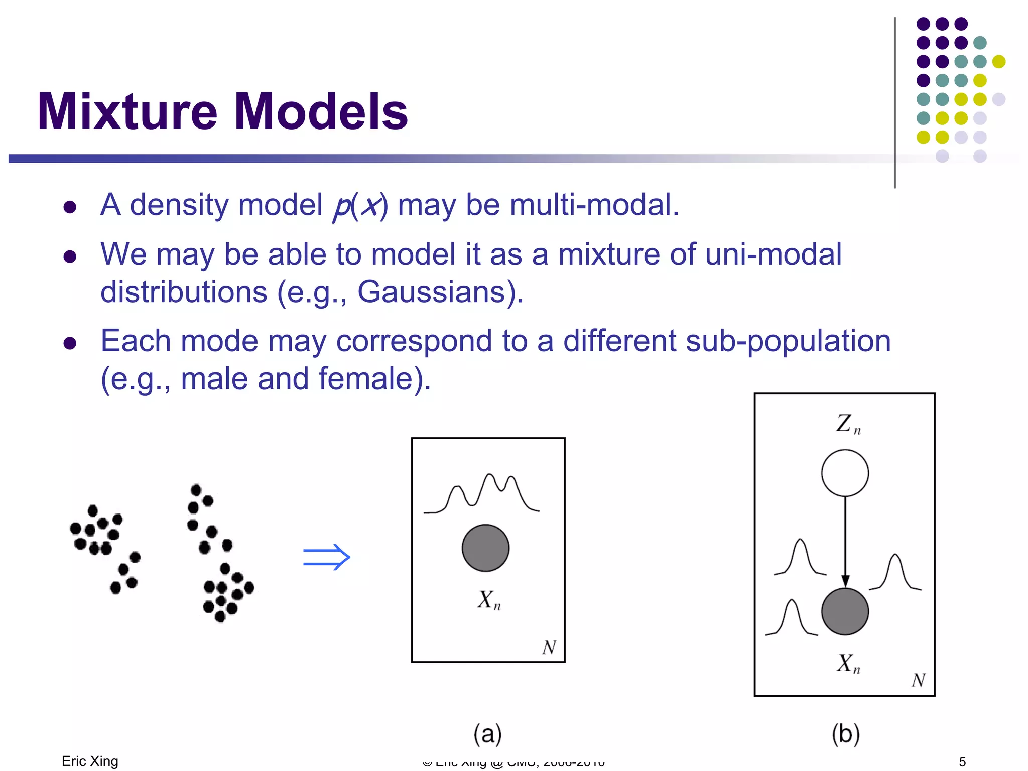
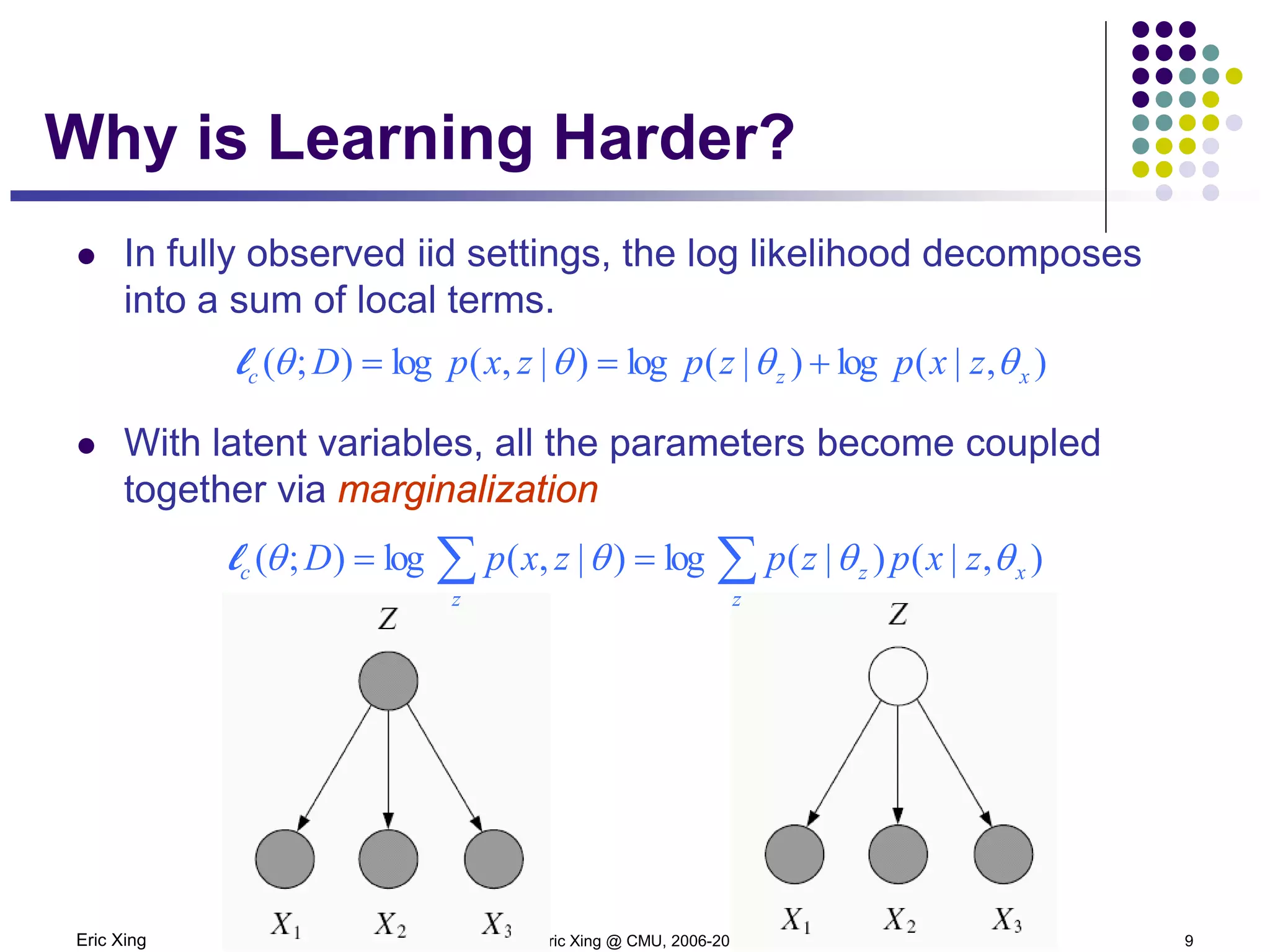
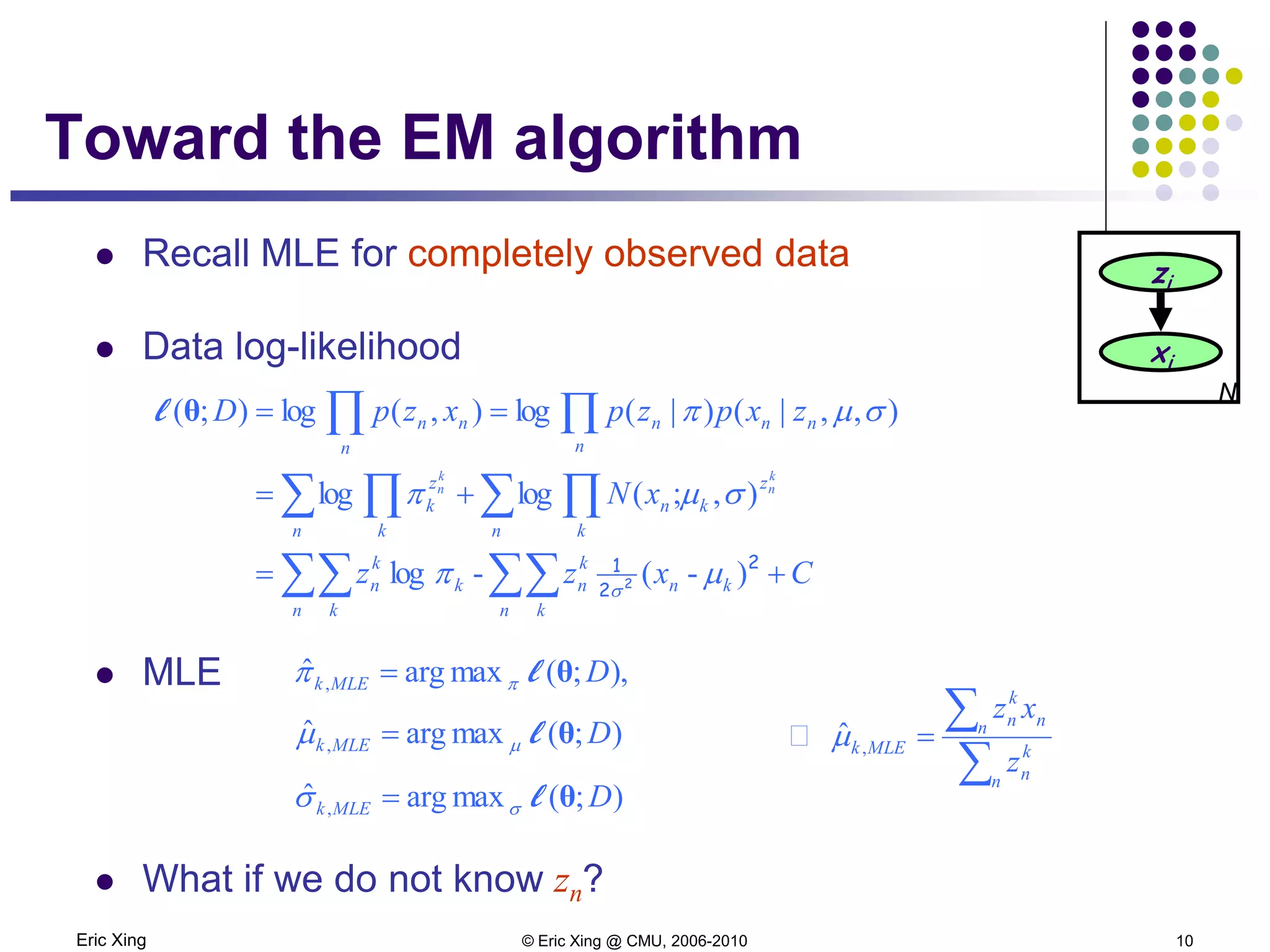
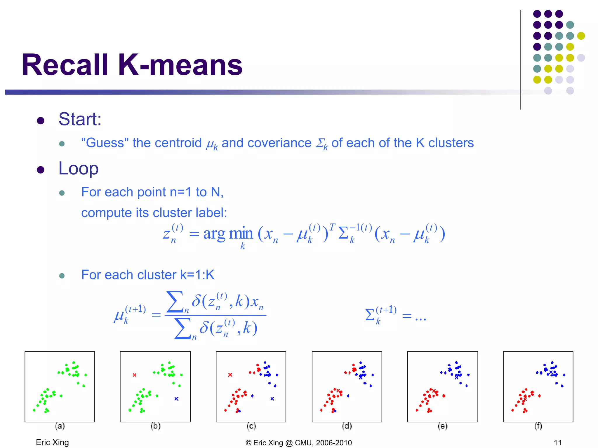
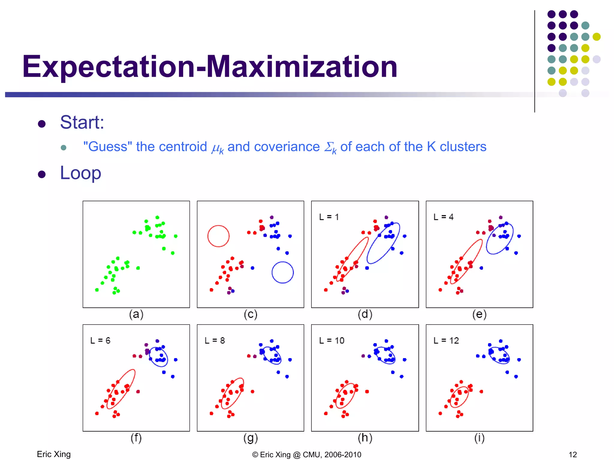
This document discusses mixture models and the Expectation Maximization (EM) algorithm. It begins by introducing mixture models like Gaussian mixture models (GMMs) which model data as a mixture of distributions. Learning the parameters of these models is difficult because the component assignments are latent variables. The EM algorithm addresses this by iteratively computing expectations of the latent variables given the current parameters (E-step) and maximizing the expected complete log likelihood (M-step). This provides a way to learn the parameters of mixture models when latent variables are involved.

![Eric Xing © Eric Xing @ CMU, 2006-2010 15
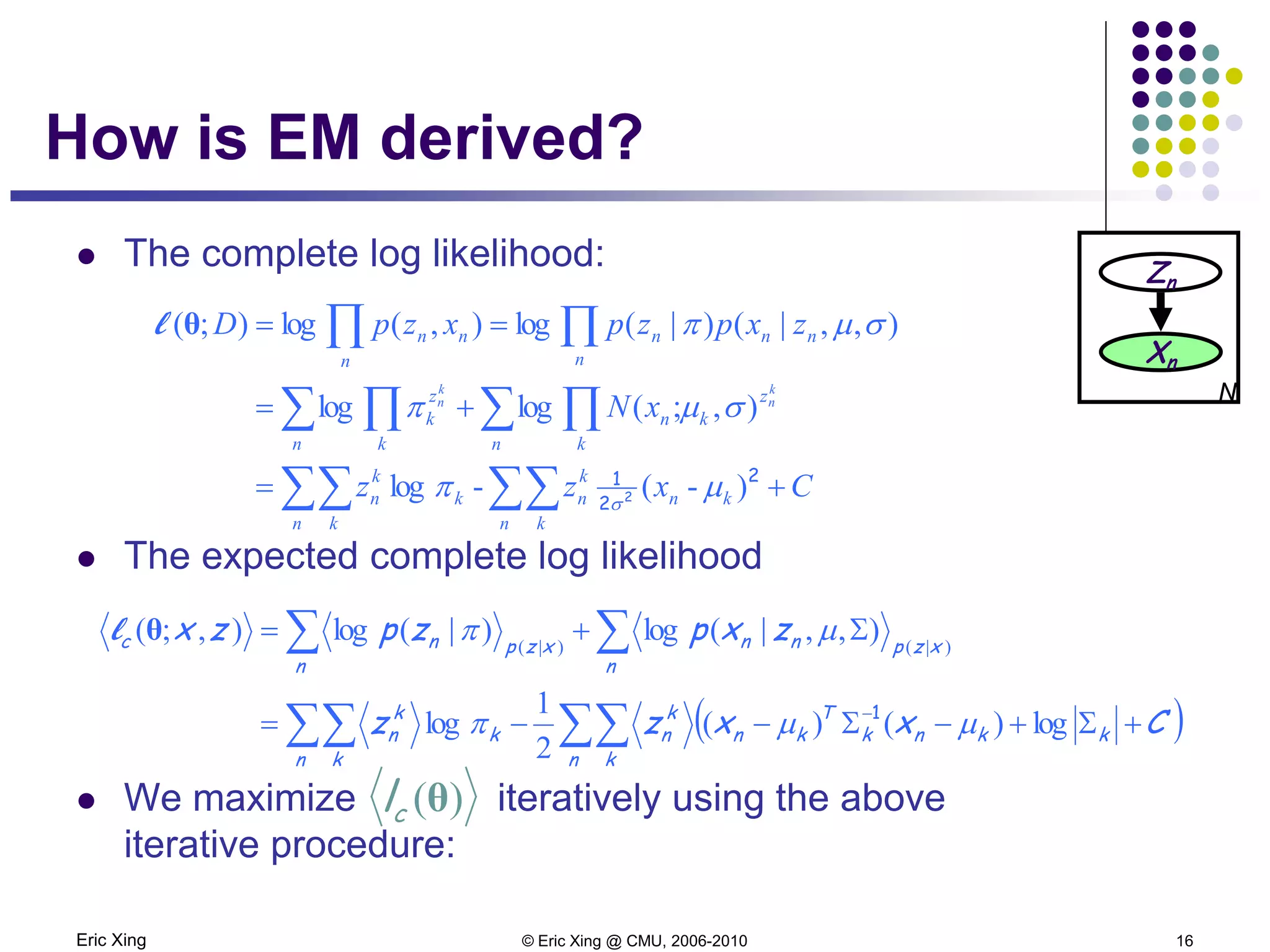
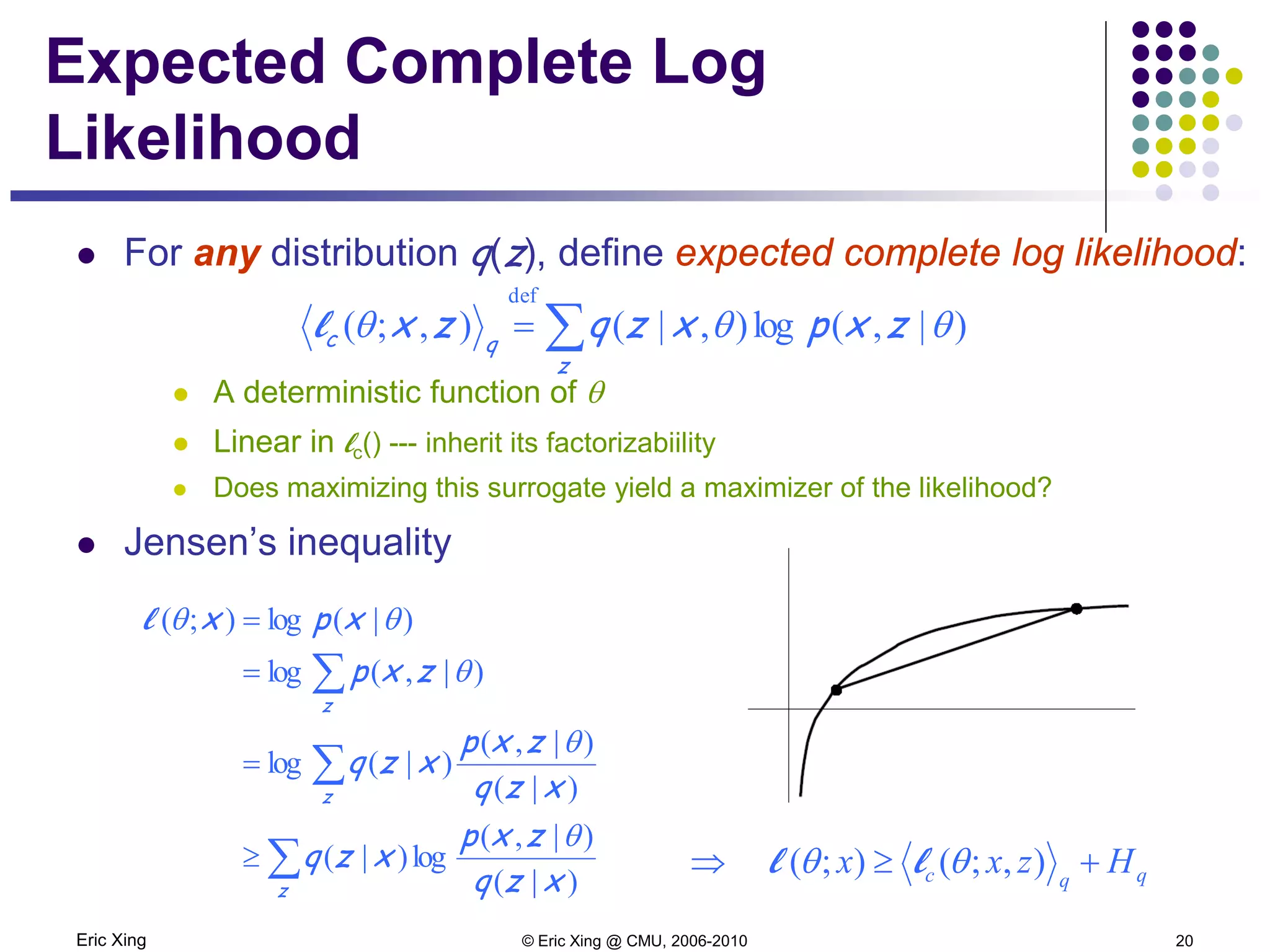
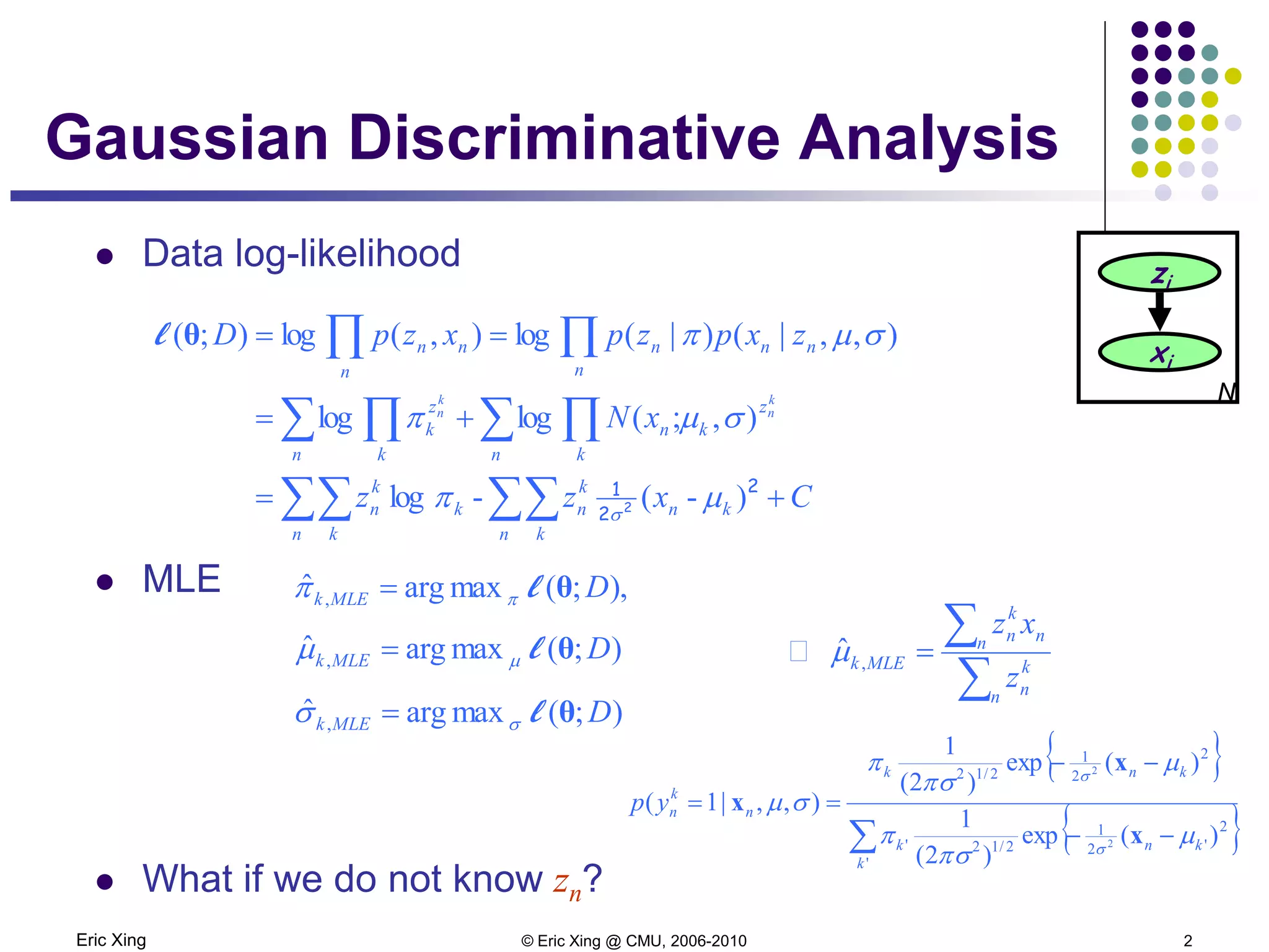
How is EM derived?
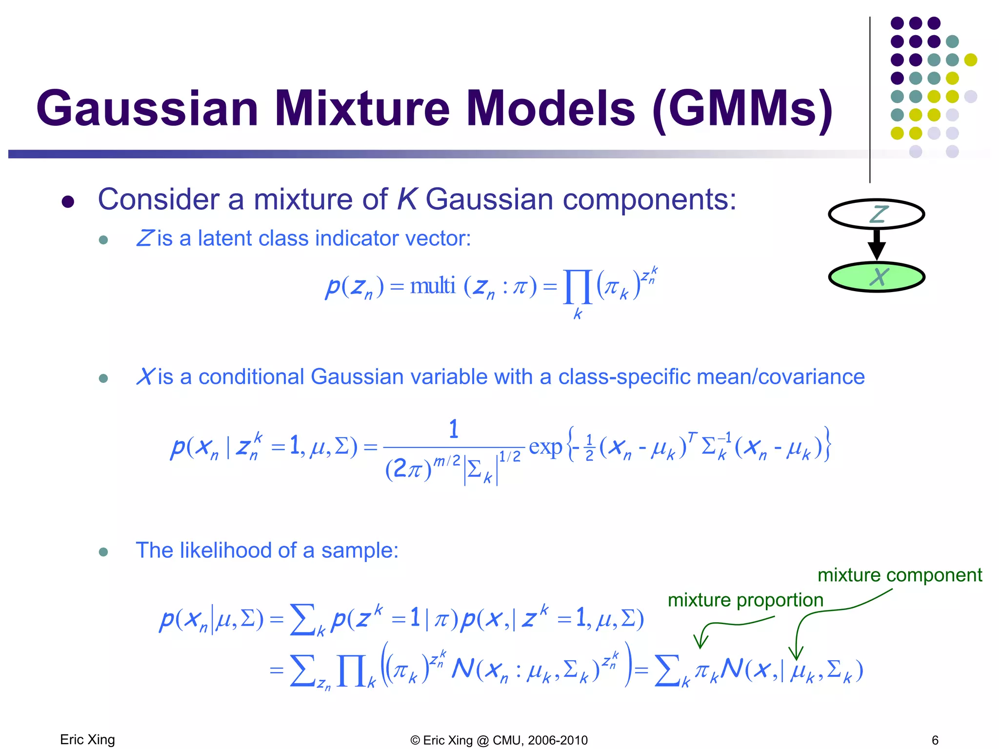
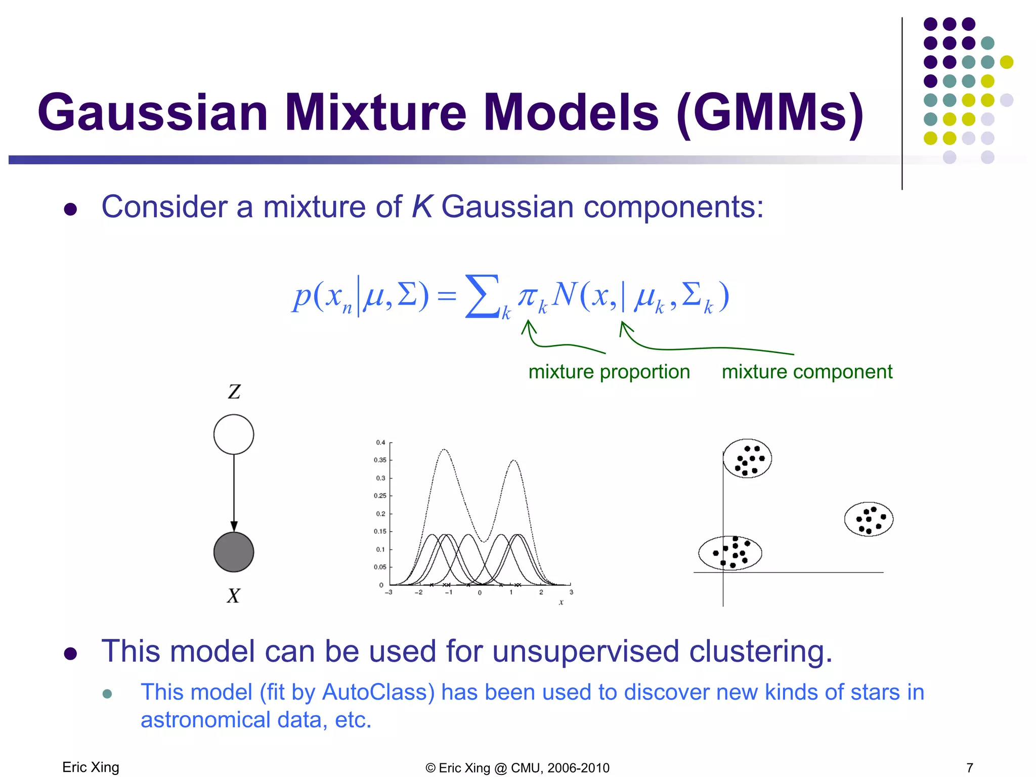
A mixture of K Gaussians:
Z is a latent class indicator vector
X is a conditional Gaussian variable with a class-specific mean/covariance
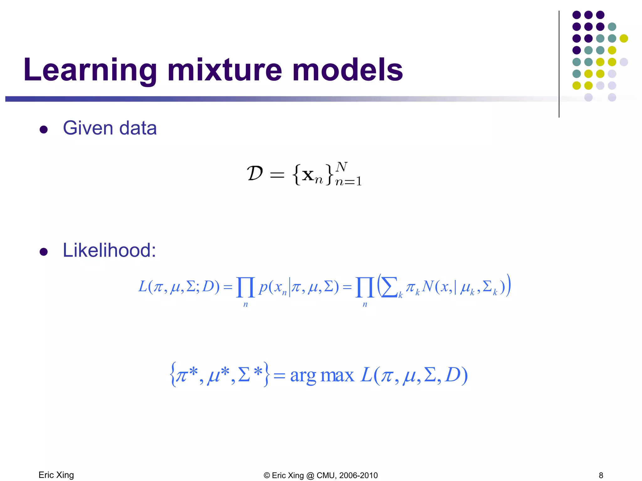
The likelihood of a sample:
The “complete” likelihood
Zn
Xn
N
( )∏):(multi)(
k
z
knn
k
n
zzp ππ ==
{ })-()-(-exp
)(
),,|( // knk
T
kn
k
m
k
nn xxzxp µµ
π
µ 1
2
1
212
2
1
1 −
Σ
Σ
=Σ=
( )( ) ∑∑ ∏
∑
Σ=Σ=
Σ===Σ
k kkkz k
z
kkn
z
k
k
k
n
k
nn
xNxN
zxpzpxp
n
k
n
k
n
),|,(),:(
),,1|,()|1(),(
µπµπ
µπµ
),|,(),,1|,()|1(),1,( kkk
k
n
k
n
k
nn xNzxpzpzxp Σ=Σ===Σ= µπµπµ
But this is itself a random variable! Not good as objective function
[ ]∏ Σ=Σ
k
z
kkknn
k
n
xNzxp ),|,(),,( µπµ](https://image.slidesharecdn.com/lecture9xing-150527174556-lva1-app6891/75/Lecture9-xing-15-2048.jpg)