Downloaded 65 times


![preliminaries
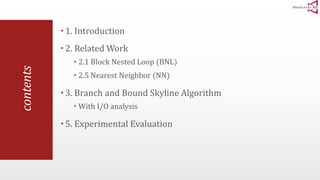
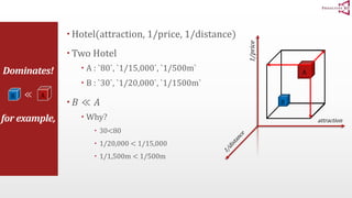
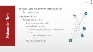
Formal definition of Dominates (≪)
Given a set of d-dimensional points 푇
We say that a point t1 ∈ 푇 DOMINATES another point t2 ∈ 푇
If and only if
∀푖 ∈ 1, 2, 3, … , 푑 , 푡1 푖 ≧ 푡2[푖]
∃푗 ∈ 1, 2, 3, … , 푑 , 푡1 푗 > 푡2[푗]
and Denoted by t2 ≪ t1
(simply saying, t1 이 이득)
Definition from http://www.comp.nus.edu.sg/~atung/publication/k_dominant.pdf
Note that
the meaning of ‘dominates’ may differ
according to type of application](https://image.slidesharecdn.com/anoptimalandprogressivealgorithmforskylinequeriesslide-141208231153-conversion-gate01/85/An-optimal-and-progressive-algorithm-for-skyline-queries-slide-6-320.jpg)

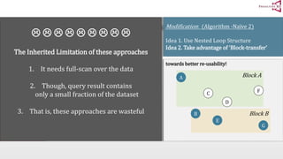


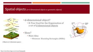
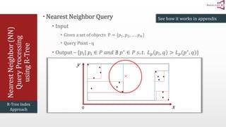
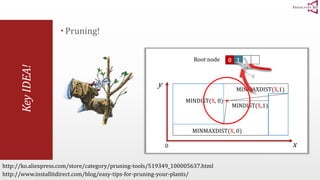


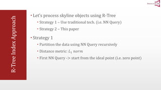

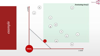
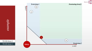

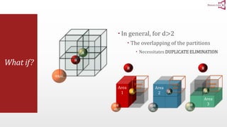


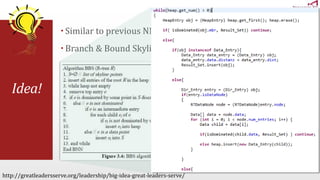
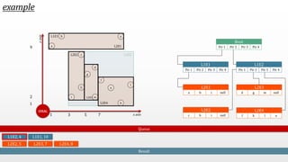
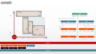

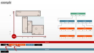
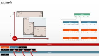
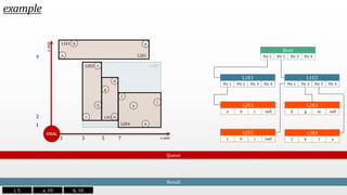

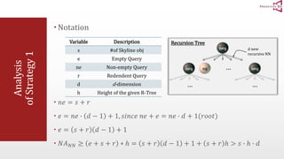

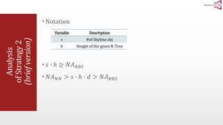

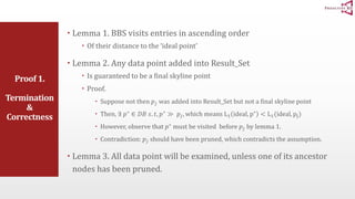
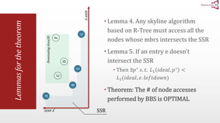
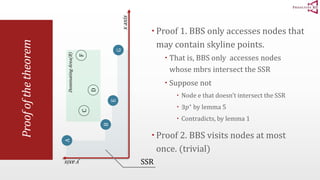


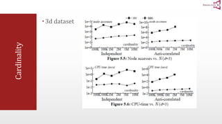

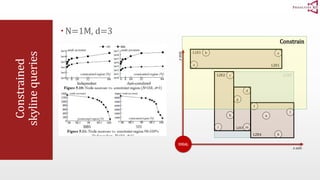

The document presents an optimal and progressive algorithm for processing skyline queries using an R-tree index. It discusses two strategies - recursive nearest neighbor queries and a branch and bound skyline algorithm. The recursive NN query approach requires additional processing to eliminate duplicate results for higher dimensions, while the branch and bound skyline algorithm prunes non-skyline points during traversal to directly generate the skyline without duplicates. The algorithm processes the R-tree in a best-first manner by maintaining a priority queue of tree nodes ordered by their minimum possible skyline size.

![Enterprise Java (November – 2018) [Choice Based | Question Paper]](https://cdn.slidesharecdn.com/ss_thumbnails/ej-cbcs-nov-2018-qp-191111054920-thumbnail.jpg?width=640&height=640&fit=bounds)