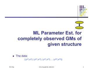
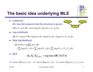
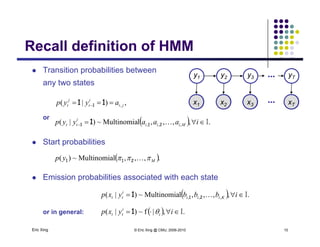
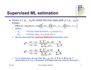
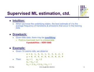
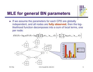
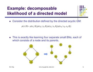
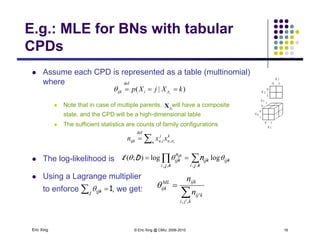
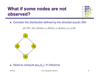
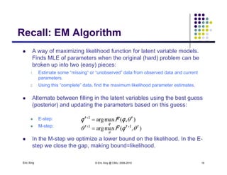
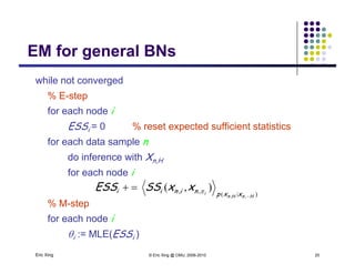
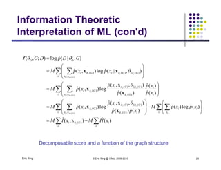
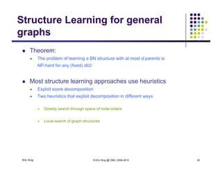
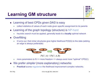
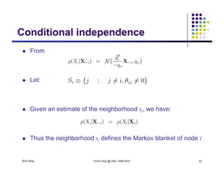
The document discusses learning graphical models from data. It describes two main tasks: inference, which is computing answers to queries about a probability distribution described by a Bayesian network, and learning, which is estimating a model from data. It provides examples of learning for completely observed models, including maximum likelihood estimation for the parameters of a conditional Gaussian model. It also discusses supervised versus unsupervised learning of hidden Markov models, and techniques for dealing with small training sets like adding pseudocounts to estimates.

![Example 1: conditional Gaussian
The completely observed model: Z
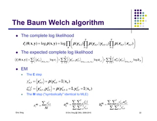
Example 1: conditional Gaussian
p y
Z is a class indicator vector
Z
X
110
2
1
∑and][where mm
ZZ
Z
Z
Z 110
∑and],,[where,
m
M
ZZ
Z
Z
zzzi M
zp )|(
21
1
All except one
of these terms
and a datum is in class i w.p. i
X i diti l G i i bl ith l ifi
m
z
m
Mi
m
zp
zp
)(
)|( 211 will be one
X is a conditional Gaussian variable with a class-specific mean
2
2
1
212 2
2
1
1 )-(-exp
)(
),,|( / m
m
xzxp
Eric Xing © Eric Xing @ CMU, 2006-2010 7
)(
m
z
m
m
xNzxp ),|(),,|( ∏ ](https://image.slidesharecdn.com/lecture12xing-150527174444-lva1-app6891/85/Lecture12-xing-7-320.jpg)
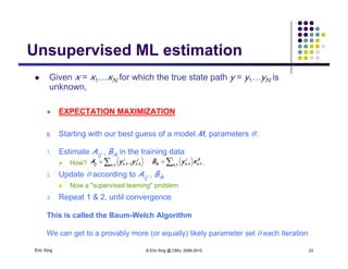
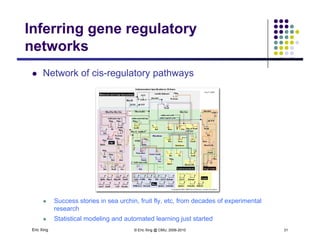
![Learning (sparse) GGMLearning (sparse) GGM
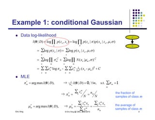
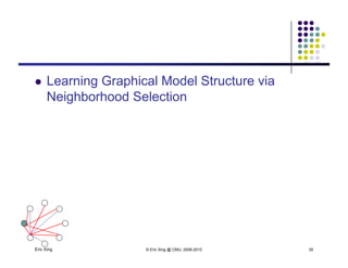
Multivariate Gaussian over all continuous expressions
{ })-()-(-exp
||)2(
1
=]),...,([ 1-
2
1
1 2
1
2
xxxxp T
n n
p
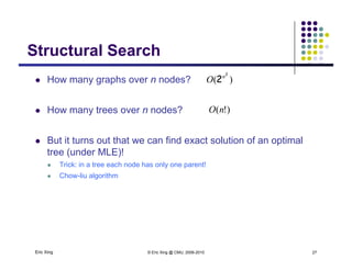
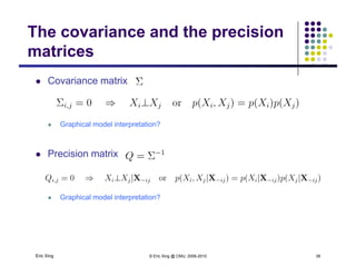
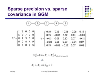
The precision matrix Q reveals the topology of the
(undirected) network
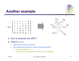
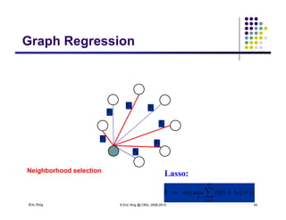
Learning Algorithm: Covariance selection
Want a sparse matrix Q
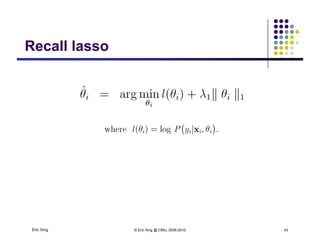
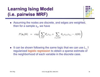
As shown in the previous slides, we can use L_1 regularized linear
regression to obtain a sparse estimate of the neighborhood of each
variable
Eric Xing © Eric Xing @ CMU, 2006-2010 48](https://image.slidesharecdn.com/lecture12xing-150527174444-lva1-app6891/85/Lecture12-xing-48-320.jpg)
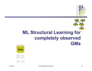
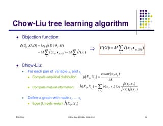
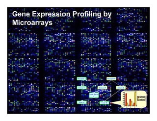
![Recent trends in GGM:Recent trends in GGM:
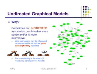
Covariance selection (classical L1-regularization based
method)
Dempster [1972]:
Sequentially pruning smallest elements
in precision matrix
method (hot !)
Meinshausen and Bühlmann [Ann. Stat.
06]:
Used LASSO regression forin precision matrix
Drton and Perlman [2008]:
Improved statistical tests for pruning
Used LASSO regression for
neighborhood selection
Banerjee [JMLR 08]:
Block sub-gradient algorithm for finding
precision matrixp
Friedman et al. [Biostatistics 08]:
Efficient fixed-point equations based
on a sub-gradient algorithm
…
Serious limitations in
ti b k d h
…
practice: breaks down when
covariance matrix is not
invertible
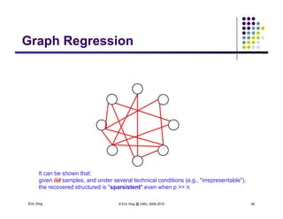
Structure learning is possible
Eric Xing © Eric Xing @ CMU, 2006-2010 49
Structure learning is possible
even when # variables > #
samples](https://image.slidesharecdn.com/lecture12xing-150527174444-lva1-app6891/85/Lecture12-xing-49-320.jpg)


![[DL輪読会]Generative Models of Visually Grounded Imagination](https://cdn.slidesharecdn.com/ss_thumbnails/20170602-170602005505-thumbnail.jpg?width=640&height=640&fit=bounds)