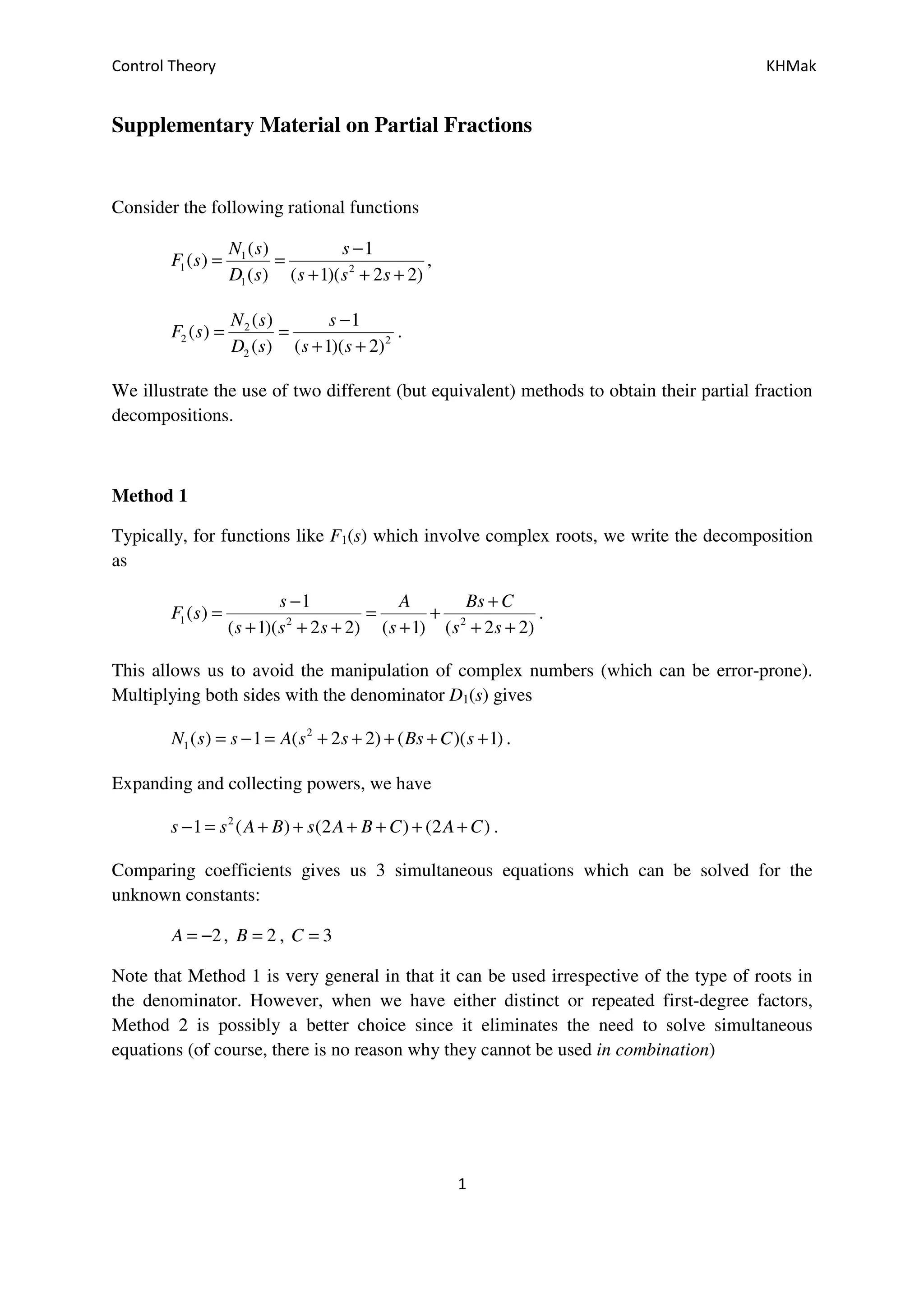
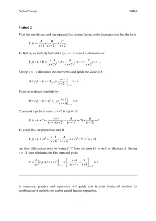
Control Theory KHMak
1
Supplementary Material on Partial Fractions
Consider the following rational functions
1
1 2
1
( ) 1
( )
( ) ( 1)( 2 2)
N s s
F s
D s s s s
−
= =
+ + +
,
2
2 2
2
( ) 1
( )
( ) ( 1)( 2)
N s s
F s
D s s s
−
= =
+ +
.
We illustrate the use of two different (but equivalent) methods to obtain their partial fraction
decompositions.
Method 1
Typically, for functions like F1(s) which involve complex roots, we write the decomposition
as
1 2 2
1
( )
( 1)( 2 2) ( 1) ( 2 2)
s A Bs C
F s
s s s s s s
− +
= = +
+ + + + + +
.
This allows us to avoid the manipulation of complex numbers (which can be error-prone).
Multiplying both sides with the denominator D1(s) gives
2
1( ) 1 ( 2 2) ( )( 1)N s s A s s Bs C s= − = + + + + + .
Expanding and collecting powers, we have
2
1 ( ) (2 ) (2 )s s A B s A B C A C− = + + + + + + .
Comparing coefficients gives us 3 simultaneous equations which can be solved for the
unknown constants:
2A = − , 2B = , 3C =
Note that Method 1 is very general in that it can be used irrespective of the type of roots in
the denominator. However, when we have either distinct or repeated first-degree factors,
Method 2 is possibly a better choice since it eliminates the need to solve simultaneous
equations (of course, there is no reason why they cannot be used in combination)
Control Theory KHMak
2
Method 2
F2(s) has one distinct and one repeated first-degree factor, so the decomposition has the form
2 2
( )
1 ( 2) 2
A B C
F s
s s s
= + +
+ + +
.
To find A, we multiply both sides by 1s + to cancel its denominator:
2 2 2
1
( ) ( 1) ( 1) ( 1)
( 2) ( 2) 2
s B C
F s s A s s
s s s
−
⋅ + = = + + + +
+ + +
.
Setting 1s = − eliminates the other terms and yields the value of A:
2 1 2
1
1
( ) ( 1) | 2
( 2)
s
s
s
A F s s
s
=−
=−
−
= ⋅ + = = −
+
.
B can be evaluated similarly by
2
2 2
2
1
( ) ( 2) | 3
( 1)
s
s
s
B F s s
s
=−
=−
−
= ⋅ + = =
+
.
C presents a problem since 2s = − is a pole of
2
1
( ) ( 2) ( 2)
( 1)( 2) ( 1) ( 2)
s A B
F s s s C
s s s s
−
⋅ + = = + + +
+ + + +
.
To avoid this, we proceed as with B
2 2
2
1
( ) ( 2) ( 2) ( 2)
( 1) ( 1)
s A
F s s s B C s
s s
−
⋅ + = = + + + +
+ +
,
but then differentiate once to “extract” C from the term Cs as well as eliminate B. Setting
2s = − then eliminates the first term and yields
2
2 2
2 2
1 1
( ) ( 2) 2
( 1) 1s s
d s
C F s s
ds s s=− =−
 −
 = ⋅ + = − + =   + + 
In summary, practice and experience will guide you in your choice of method (or
combination of methods) to use for partial fraction expansion.

Partial fractions

  • 1.
    Control Theory KHMak 1 SupplementaryMaterial on Partial Fractions Consider the following rational functions 1 1 2 1 ( ) 1 ( ) ( ) ( 1)( 2 2) N s s F s D s s s s − = = + + + , 2 2 2 2 ( ) 1 ( ) ( ) ( 1)( 2) N s s F s D s s s − = = + + . We illustrate the use of two different (but equivalent) methods to obtain their partial fraction decompositions. Method 1 Typically, for functions like F1(s) which involve complex roots, we write the decomposition as 1 2 2 1 ( ) ( 1)( 2 2) ( 1) ( 2 2) s A Bs C F s s s s s s s − + = = + + + + + + + . This allows us to avoid the manipulation of complex numbers (which can be error-prone). Multiplying both sides with the denominator D1(s) gives 2 1( ) 1 ( 2 2) ( )( 1)N s s A s s Bs C s= − = + + + + + . Expanding and collecting powers, we have 2 1 ( ) (2 ) (2 )s s A B s A B C A C− = + + + + + + . Comparing coefficients gives us 3 simultaneous equations which can be solved for the unknown constants: 2A = − , 2B = , 3C = Note that Method 1 is very general in that it can be used irrespective of the type of roots in the denominator. However, when we have either distinct or repeated first-degree factors, Method 2 is possibly a better choice since it eliminates the need to solve simultaneous equations (of course, there is no reason why they cannot be used in combination)
  • 2.
    Control Theory KHMak 2 Method2 F2(s) has one distinct and one repeated first-degree factor, so the decomposition has the form 2 2 ( ) 1 ( 2) 2 A B C F s s s s = + + + + + . To find A, we multiply both sides by 1s + to cancel its denominator: 2 2 2 1 ( ) ( 1) ( 1) ( 1) ( 2) ( 2) 2 s B C F s s A s s s s s − ⋅ + = = + + + + + + + . Setting 1s = − eliminates the other terms and yields the value of A: 2 1 2 1 1 ( ) ( 1) | 2 ( 2) s s s A F s s s =− =− − = ⋅ + = = − + . B can be evaluated similarly by 2 2 2 2 1 ( ) ( 2) | 3 ( 1) s s s B F s s s =− =− − = ⋅ + = = + . C presents a problem since 2s = − is a pole of 2 1 ( ) ( 2) ( 2) ( 1)( 2) ( 1) ( 2) s A B F s s s C s s s s − ⋅ + = = + + + + + + + . To avoid this, we proceed as with B 2 2 2 1 ( ) ( 2) ( 2) ( 2) ( 1) ( 1) s A F s s s B C s s s − ⋅ + = = + + + + + + , but then differentiate once to “extract” C from the term Cs as well as eliminate B. Setting 2s = − then eliminates the first term and yields 2 2 2 2 2 1 1 ( ) ( 2) 2 ( 1) 1s s d s C F s s ds s s=− =−  −  = ⋅ + = − + =   + +  In summary, practice and experience will guide you in your choice of method (or combination of methods) to use for partial fraction expansion.