Downloaded 569 times
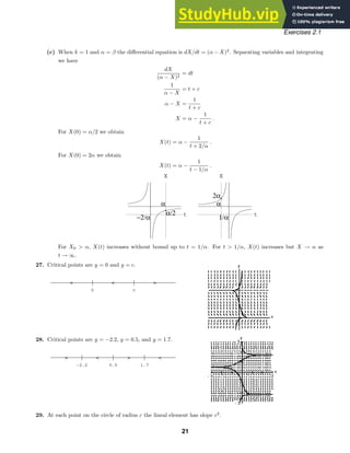
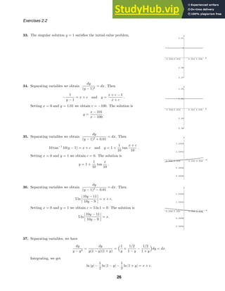
![-4 -2 2 4 x
-4
-2
2
4
y
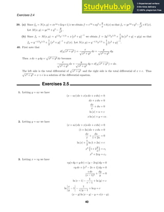
Exercises 1.1
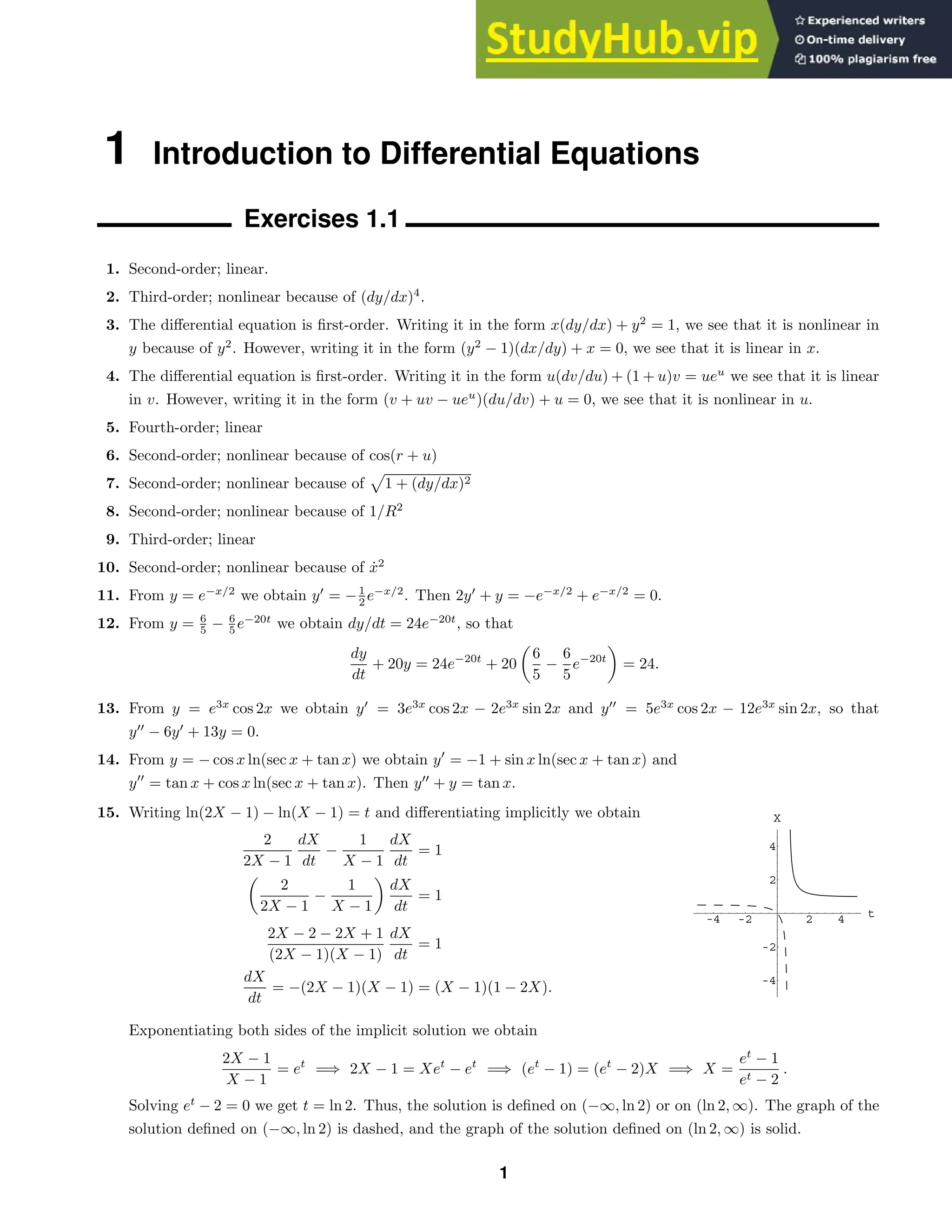
16. Implicitly differentiating the solution we obtain
−2x2 dy
dx
− 4xy + 2y
dy
dx
= 0 =⇒ −x2
dy − 2xy dx + y dy = 0
=⇒ 2xy dx + (x2
− y)dy = 0.
Using the quadratic formula to solve y2
− 2x2
y − 1 = 0 for y, we get
y =
2x2
±
√
4x4 + 4
/2 = x2
±
√
x4 + 1 . Thus, two explicit solutions are
y1 = x2
+
√
x4 + 1 and y2 = x2
−
√
x4 + 1 . Both solutions are defined on
(−∞, ∞). The graph of y1(x) is solid and the graph of y2 is dashed.
17. Differentiating P = c1et
/ (1 + c1et
) we obtain
dP
dt
=
(1 + c1et
) c1et
− c1et
· c1et
(1 + c1et)
2
=
c1et
1 + c1et
[(1 + c1et
) − c1et
]
1 + c1et
= P(1 − P).
18. Differentiating y = e−x2
x
0
et2
dt + c1e−x2
we obtain
y
= e−x2
ex2
− 2xe−x2
x
0
et2
dt − 2c1xe−x2
= 1 − 2xe−x2
x
0
et2
dt − 2c1xe−x2
.
Substituting into the differential equation, we have
y
+ 2xy = 1 − 2xe−x2
x
0
et2
dt − 2c1xe−x2
+ 2xe−x2
x
0
et2
dt + 2c1xe−x2
= 1.
19. From y = c1e2x
+ c2xe2x
we obtain
dy
dx
= (2c1 + c2)e2x
+ 2c2xe2x
and
d2
y
dx2
= (4c1 + 4c2)e2x
+ 4c2xe2x
, so that
d2
y
dx2
− 4
dy
dx
+ 4y = (4c1 + 4c2 − 8c1 − 4c2 + 4c1)e2x
+ (4c2 − 8c2 + 4c2)xe2x
= 0.
20. From y = c1x−1
+ c2x + c3x ln x + 4x2
we obtain
dy
dx
= −c1x−2
+ c2 + c3 + c3 ln x + 8x,
d2
y
dx2
= 2c1x−3
+ c3x−1
+ 8,
and
d3
y
dx3
= −6c1x−4
− c3x−2
,
so that
x3 d3
y
dx3
+ 2x2 d2
y
dx2
− x
dy
dx
+ y
= (−6c1 + 4c1 + c1 + c1)x−1
+ (−c3 + 2c3 − c2 − c3 + c2)x
+ (−c3 + c3)x ln x + (16 − 8 + 4)x2
= 12x2
.
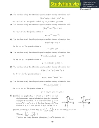
21. From y =
−x2
, x 0
x2
, x ≥ 0
we obtain y
=
−2x, x 0
2x, x ≥ 0
so that xy
− 2y = 0.
2](https://image.slidesharecdn.com/advancedengineeringmathematicssolutionsmanual-230807162553-1916df96/85/Advanced-Engineering-Mathematics-Solutions-Manual-pdf-2-320.jpg)
![Exercises 1.1
22. The function y(x) is not continuous at x = 0 since lim
x→0−
y(x) = 5 and lim
x→0+
y(x) = −5. Thus, y
(x) does not
exist at x = 0.
23. From x = e−2t
+ 3e6t
and y = −e−2t
+ 5e6t
we obtain
dx
dt
= −2e−2t
+ 18e6t
and
dy
dt
= 2e−2t
+ 30e6t
.
Then
x + 3y = (e−2t
+ 3e6t
) + 3(−e−2t
+ 5e6t
)
= −2e−2t
+ 18e6t
=
dx
dt
and
5x + 3y = 5(e−2t
+ 3e6t
) + 3(−e−2t
+ 5e6t
)
= 2e−2t
+ 30e6t
=
dy
dt
.
24. From x = cos 2t + sin 2t + 1
5 et
and y = − cos 2t − sin 2t − 1
5 et
we obtain
dx
dt
= −2 sin 2t + 2 cos 2t +
1
5
et
and
dy
dt
= 2 sin 2t − 2 cos 2t −
1
5
et
and
d2
x
dt2
= −4 cos 2t − 4 sin 2t +
1
5
et
and
d2
y
dt2
= 4 cos 2t + 4 sin 2t −
1
5
et
.
Then
4y + et
= 4(− cos 2t − sin 2t −
1
5
et
) + et
= −4 cos 2t − 4 sin 2t +
1
5
et
=
d2
x
dt2
and
4x − et
= 4(cos 2t + sin 2t +
1
5
et
) − et
= 4 cos 2t + 4 sin 2t −
1
5
et
=
d2
y
dt2
.
25. An interval on which tan 5t is continuous is −π/2 5t π/2, so 5 tan 5t will be a solution on (−π/10, π/10).
26. For (1 − sin t)−1/2
to be continuous we must have 1 − sin t 0 or sin t 1. Thus, (1 − sin t)−1/2
will be a
solution on (π/2, 5π/2).
27. (y
)2
+ 1 = 0 has no real solution.
28. The only solution of (y
)2
+ y2
= 0 is y = 0, since if y = 0, y2
0 and (y
)2
+ y2
≥ y2
0.
29. The first derivative of f(t) = et
is et
. The first derivative of f(t) = ekt
is kekt
. The differential equations are
y
= y and y
= ky, respectively.
30. Any function of the form y = cet
or y = ce−t
is its own second derivative. The corresponding differential
equation is y
− y = 0. Functions of the form y = c sin t or y = c cos t have second derivatives that are the
negatives of themselves. The differential equation is y
+ y = 0.
31. Since the nth derivative of φ(x) must exist if φ(x) is a solution of the nth order differential equation, all lower-
order derivatives of φ(x) must exist and be continuous. [Recall that a differentiable function is continuous.]
32. Solving the system
c1y1(0) + c2y2(0) = 2
c1y
1(0) + c2y
2(0) = 0
3](https://image.slidesharecdn.com/advancedengineeringmathematicssolutionsmanual-230807162553-1916df96/85/Advanced-Engineering-Mathematics-Solutions-Manual-pdf-3-320.jpg)
![Exercises 1.1
for c1 and c2 we get
c1 =
2y
2(0)
y1(0)y
2(0) − y
1(0)y2(0)
and c2 = −
2y
1(0)
y1(0)y
2(0) − y
1(0)y2(0)
.
Thus, a particular solution is
y =
2y
2(0)
y1(0)y
2(0) − y
1(0)y2(0)
y1 −
2y
1(0)
y1(0)y
2(0) − y
1(0)y2(0)
y2,
where we assume that y1(0)y
2(0) − y
1(0)y2(0) = 0.
33. For the first-order differential equation integrate f(x). For the second-order differential equation integrate twice.
In the latter case we get y = ( f(t)dt)dt + c1t + c2.
34. Solving for y
using the quadratic formula we obtain the two differential equations
y
=
1
t
2 + 2
1 + 3t6 and y
=
1
t
2 − 2
1 + 3t6 ,
so the differential equation cannot be put in the form dy/dt = f(t, y).
35. The differential equation yy
− ty = 0 has normal form dy/dt = t. These are not equivalent because y = 0 is a
solution of the first differential equation but not a solution of the second.
36. Differentiating we get y
= c1 + 3c2t2
and y
= 6c2t. Then c2 = y
/6t and c1 = y
− ty
/2, so
y =
y
−
ty
2
t +
y
6t
t3
= ty
−
1
3
t2
y
and the differential equation is t2
y
− 3ty
+ 3y = 0.
37. (a) From y = emt
we obtain y
= memt
. Then y
+ 2y = 0 implies
memt
+ 2emt
= (m + 2)emt
= 0.
Since emt
0 for all t, m = −2. Thus y = e−2t
is a solution.
(b) From y = emt
we obtain y
= memt
and y
= m2
emt
. Then y
− 5y
+ 6y = 0 implies
m2
emt
− 5memt
+ 6emt
= (m − 2)(m − 3)emt
= 0.
Since emt
0 for all t, m = 2 and m = 3. Thus y = e2t
and y = e3t
are solutions.
(c) From y = tm
we obtain y
= mtm−1
and y
= m(m − 1)tm−2
. Then ty
+ 2y
= 0 implies
tm(m − 1)tm−2
+ 2mtm−1
= [m(m − 1) + 2m]tm−1
= (m2
+ m)tm−1
= m(m + 1)tm−1
= 0.
Since tm−1
0 for t 0, m = 0 and m = −1. Thus y = 1 and y = t−1
are solutions.
(d) From y = tm
we obtain y
= mtm−1
and y
= m(m − 1)tm−2
. Then t2
y
− 7ty
+ 15y = 0 implies
t2
m(m − 1)tm−2
− 7tmtm−1
+ 15tm
= [m(m − 1) − 7m + 15]tm
= (m2
− 8m + 15)tm
= (m − 3)(m − 5)tm
= 0.
Since tm
0 for t 0, m = 3 and m = 5. Thus y = t3
and y = t5
are solutions.
38. When g(t) = 0, y = 0 is a solution of a linear equation.
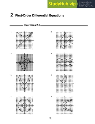
39. (a) Solving (10 − 5y)/3x = 0 we see that y = 2 is a constant solution.
(b) Solving y2
+ 2y − 3 = (y + 3)(y − 1) = 0 we see that y = −3 and y = 1 are constant solutions.
(c) Since 1/(y − 1) = 0 has no solutions, the differential equation has no constant solutions.
4](https://image.slidesharecdn.com/advancedengineeringmathematicssolutionsmanual-230807162553-1916df96/85/Advanced-Engineering-Mathematics-Solutions-Manual-pdf-4-320.jpg)
![y=a b
y=0
x
y
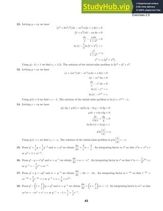
Exercises 1.1
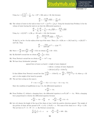
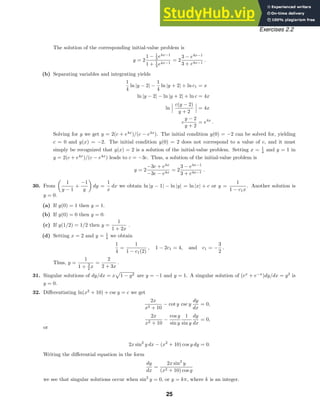
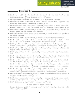
(b) Since dy/dx = y(a − by) 0 for 0 y a/b, y = φ(x) is increasing on this interval. Since dy/dx 0 for
y 0 or y a/b, y = φ(x) is decreasing on these intervals.
(c) Using implicit differentiation we compute
d2
y
dx2
= y(−by
) + y
(a − by) = y
(a − 2by).
Solving d2
y/dx2
= 0 we obtain y = a/2b. Since d2
y/dx2
0 for 0 y a/2b and d2
y/dx2
0 for
a/2b y a/b, the graph of y = φ(x) has a point of inflection at y = a/2b.
(d)
48. (a) In Mathematica use
Clear[y]
y[x ]:= x Exp[5x] Cos[2x]
y[x]
y''''[x] − 20 y'''[x] + 158 y''[x] − 580 y'[x] + 841 y[x] // Simplify
(b) In Mathematica use
Clear[y]
y[x ]:= 20 Cos[5 Log[x]]/x − 3 Sin[5 Log[x]]/x
y[x]
xˆ3 y'''[x] + 2xˆ2 y''[x] + 20 x y'[x] − 78 y[x] // Simplify
Exercises 1.2
1. Solving −
1
3
=
1
1 + c1
we get c1 = −4. The solution is y =
1
1 − 4e−t
.
2. Solving 2 =
1
1 + c1e
we get c1 = −
1
2
e−1
. The solution is y =
2
2 − e−(t+1)
.
3. Using x
= −c1 sin t + c2 cos t we obtain c1 = −1 and c2 = 8. The solution is x = − cos t + 8 sin t.
4. Using x
= −c1 sin t + c2 cos t we obtain c2 = 0 and −c1 = 1. The solution is x = − cos t.
5. Using x
= −c1 sin t + c2 cos t we obtain
√
3
2
c1 +
1
2
c2 =
1
2
−
1
2
c1 +
√
3
2
c2 = 0.
Solving we find c1 =
√
3
4
and c2 =
1
4
. The solution is x =
√
3
4
cos t +
1
4
sin t.
6](https://image.slidesharecdn.com/advancedengineeringmathematicssolutionsmanual-230807162553-1916df96/85/Advanced-Engineering-Mathematics-Solutions-Manual-pdf-6-320.jpg)


![(x,y)
x
y
α
α
θ
θ
θ
φ
x
y
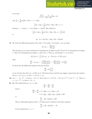
Exercises 1.3
Thus, the differential equation is
x
d2
x
dt
+
dx
dt
2
+ 32x = 160.
20. The force is the weight of the chain, 2L, so by Newton’s second law,
d
dt
[mv] = 2L. Since the mass of the portion
of chain off the ground is m = 2(L − x)/g, we have
d
dt
2(L − x)
g
v
= 2L or (L − x)
dv
dt
+ v −
dx
dt
= Lg.
Thus, the differential equation is
(L − x)
d2
x
dt2
−
dx
dt
2
= Lg.
21. From g = k/R2
we find k = gR2
. Using a = d2
r/dt2
and the fact that the positive direction is upward we get
d2
r
dt2
= −a = −
k
r2
= −
gR2
r2
or
d2
r
dt2
+
gR2
r2
= 0.
22. The gravitational force on m is F = −kMrm/r2
. Since Mr = 4πδr3
/3 and M = 4πδR3
/3 we have Mr = r3
M/R3
and
F = −k
Mrm
r2
= −k
r3
Mm/R3
r2
= −k
mM
R3
r.
Now from F = ma = d2
r/dt2
we have
m
d2
r
dt2
= −k
mM
R3
r or
d2
r
dt2
= −
kM
R3
r.
23. The differential equation is
dA
dt
= k(M − A).
24. The differential equation is
dA
dt
= k1(M − A) − k2A.
25. The differential equation is x
(t) = r − kx(t) where k 0.
26. By the Pythagorean Theorem the slope of the tangent line is y
=
−y
s2 − y2
.
27. We see from the figure that 2θ + α = π. Thus
y
−x
= tan α = tan(π − 2θ) = − tan 2θ = −
2 tan θ
1 − tan2
θ
.
Since the slope of the tangent line is y
= tan θ we have y/x = 2y
[1 − (y
)2
] or
y − y(y
)2
= 2xy
, which is the quadratic equation y(y
)2
+ 2xy
− y = 0 in y
.
Using the quadratic formula we get
y
=
−2x ±
4x2 + 4y2
2y
=
−x ±
x2 + y2
y
.
Since dy/dx 0, the differential equation is
dy
dx
=
−x +
x2 + y2
y
or y
dy
dx
−
x2 + y2 + x = 0.
28. The differential equation is dP/dt = kP, so from Problem 29 in Exercises 1.1, P = ekt
, and a one-parameter
family of solutions is P = cekt
.
12](https://image.slidesharecdn.com/advancedengineeringmathematicssolutionsmanual-230807162553-1916df96/85/Advanced-Engineering-Mathematics-Solutions-Manual-pdf-12-320.jpg)
![Exercises 1.3
29. The differential equation in (3) is dT/dt = k(T − Tm). When the body is cooling, T Tm, so T − Tm 0.
Since T is decreasing, dT/dt 0 and k 0. When the body is warming, T Tm, so T − Tm 0. Since T is
increasing, dT/dt 0 and k 0.
30. The differential equation in (8) is dA/dt = 6 − A/100. If A(t) attains a maximum, then dA/dt = 0 at this time
and A = 600. If A(t) continues to increase without reaching a maximum then A
(t) 0 for t 0 and A cannot
exceed 600. In this case, if A
(t) approaches 0 as t increases to infinity, we see that A(t) approaches 600 as t
increases to infinity.
31. This differential equation could describe a population that undergoes periodic fluctuations.
32. (1):
dP
dt
= kP is linear (2):
dA
dt
= kA is linear
(3):
dT
dt
= k(T − Tm) is linear (5):
dx
dt
= kx(n + 1 − x) is nonlinear
(6):
dX
dt
= k(α − X)(β − X) is nonlinear (8):
dA
dt
= 6 −
A
100
is linear
(10):
dh
dt
= −
Ah
Aw
2gh is nonlinear (11): L
d2
q
dt2
+ R
dq
dt
+
1
C
q = E(t) is linear
(12):
d2
s
dt2
= −g is linear (14): m
dv
dt
= mg − kv is linear
(15): m
d2
s
dt2
+ k
ds
dt
= mg is linear (16):
d2
x
dt2
−
64
L
x = 0 is linear
33. From Problem 21, d2
r/dt2
= −gR2
/r2
. Since R is a constant, if r = R + s, then d2
r/dt2
= d2
s/dt2
and, using
a Taylor series, we get
d2
s
dt2
= −g
R2
(R + s)2
= −gR2
(R + s)−2
≈ −gR2
[R−2
− 2sR−3
+ · · · ] = −g +
2gs
R3
+ · · · .
Thus, for R much larger than s, the differential equation is approximated by d2
s/dt2
= −g.
34. If ρ is the mass density of the raindrop, then m = ρV and
dm
dt
= ρ
dV
dt
= ρ
d
dt
4
3
πr3
= ρ 4πr2 dr
dt
= ρS
dr
dt
.
If dr/dt is a constant, then dm/dt = kS where ρ dr/dt = k or dr/dt = k/ρ. Since the radius is decreasing,
k 0. Solving dr/dt = k/ρ we get r = (k/ρ)t + c0. Since r(0) = r0, c0 = r0 and r = kt/ρ + r0.
From Newton’s second law,
d
dt
[mv] = mg, where v is the velocity of the raindrop. Then
m
dv
dt
+ v
dm
dt
= mg or ρ
4
3
πr3 dv
dt
+ v(k4πr2
) = ρ
4
3
πr3
g.
Dividing by 4ρπr3
/3 we get
dv
dt
+
3k
ρr
v = g or
dv
dt
+
3k/ρ
kt/ρ + r0
v = g, k 0.
35. We assume that the plow clears snow at a constant rate of k cubic miles per hour. Let t be the time in hours
after noon, x(t) the depth in miles of the snow at time t, and y(t) the distance the plow has moved in t hours.
Then dy/dt is the velocity of the plow and the assumption gives
wx
dy
dt
= k
13](https://image.slidesharecdn.com/advancedengineeringmathematicssolutionsmanual-230807162553-1916df96/85/Advanced-Engineering-Mathematics-Solutions-Manual-pdf-13-320.jpg)
![Exercises 1.3
where w is the width of the plow. Each side of this equation simply represents the volume of snow plowed in
one hour. Now let t0 be the number of hours before noon when it started snowing and let s be the constant rate
in miles per hour at which x increases. Then for t −t0, x = s(t + t0). The differential equation then becomes
dy
dt
=
k
ws
1
t + t0
.
Integrating we obtain
y =
k
ws
[ ln(t + t0) + c ]
where c is a constant. Now when t = 0, y = 0 so c = − ln t0 and
y =
k
ws
ln
1 +
t
t0
.
Finally, from the fact that when t = 1, y = 2 and when t = 2, y = 3, we obtain
1 +
2
t0
2
=
1 +
1
t0
3
.
Expanding and simplifying gives t2
0 + t0 − 1 = 0. Since t0 0, we find t0 ≈ 0.618 hours ≈ 37 minutes. Thus it
started snowing at about 11:23 in the morning.
Chapter 1 Review Exercises
1.
d
dx
c1
x
= −
c1
x2
= −
c1/x
x
;
dy
dx
= −
y
x
2.
d
dx
(5 + c1e−2x
) = −2c1e−2x
= −2(5 + c1e−2x
− 5);
dy
dx
= −2(y − 5) or
dy
dx
= −2y + 10
3.
d
dx
(c1 cos kx + c2 sin kx) = −kc1 sin kx + kc2 cos kx;
d2
dx2
(c1 cos kx + c2 sin kx) = −k2
c1 cos kx − k2
c2 sin kx = −k2
(c1 cos kx + c2 sin kx);
d2
y
dx2
= −k2
y or
d2
y
dx2
+ k2
y = 0
4.
d
dx
(c1 cosh kx + c2 sinh kx) = kc1 sinh kx + kc2 cosh kx;
d2
dx2
(c1 cosh kx + c2 sinh kx) = k2
c1 cosh kx + k2
c2 sinh kx = k2
(c1 cosh kx + c2 sinh kx);
d2
y
dx2
= k2
y or
d2
y
dx2
− k2
y = 0
5. y
= c1ex
+ c2xex
+ c2ex
; y
= c1ex
+ c2xex
+ 2c2ex
;
y
+ y = 2(c1ex
+ c2xex
) + 2c2ex
= 2(c1ex
+ c2xex
+ c2ex
) = 2y
; y
− 2y
+ y = 0
6. y
= −c1ex
sin x + c1ex
cos x + c2ex
cos x + c2ex
sin x;
y
= −c1ex
cos x − c1ex
sin x − c1ex
sin x + c1ex
cos x − c2ex
sin x + c2ex
cos x + c2ex
cos x + c2ex
sin x
= −2c1ex
sin x + 2c2ex
cos x;
y
− 2y
= −2c1ex
cos x − 2c2ex
sin x = −2y; y
− 2y
+ 2y = 0
7. a,d 8. c 9. b 10. a,c 11. b 12. a,b,d
13. A few solutions are y = 0, y = c, and y = ex
.
14](https://image.slidesharecdn.com/advancedengineeringmathematicssolutionsmanual-230807162553-1916df96/85/Advanced-Engineering-Mathematics-Solutions-Manual-pdf-14-320.jpg)
![-3 -2 -1 1 2 3 x
-3
-2
-1
1
2
3
y
-3 -2 -1 1 2 3 x
-3
-2
-1
1
2
3
y
Chapter 1 Review Exercises
14. Easy solutions to see are y = 0 and y = 3.
15. The slope of the tangent line at (x, y) is y
, so the differential equation is y
= x2
+ y2
.
16. The rate at which the slope changes is dy
/dx = y
, so the differential equation is y
= −y
or y
+ y
= 0.
17. (a) The domain is all real numbers.
(b) Since y
= 2/3x1/3
, the solution y = x2/3
is undefined at x = 0. This function is a solution of the differential
equation on (−∞, 0) and also on (0, ∞).
18. (a) Differentiating y2
− 2y = x2
− x + c we obtain 2yy
− 2y
= 2x − 1 or (2y − 2)y
= 2x − 1.
(b) Setting x = 0 and y = 1 in the solution we have 1 − 2 = 0 − 0 + c or c = −1. Thus, a solution of the
initial-value problem is y2
− 2y = x2
− x − 1.
(c) Using the quadratic formula to solve y2
− 2y − (x2
− x − 1) = 0 we get y = (2 ±
4 + 4(x2 − x − 1) )/2
= 1±
√
x2 − x = 1±
x(x − 1) . Since x(x−1) ≥ 0 for x ≤ 0 or x ≥ 1, we see that neither y = 1+
x(x − 1)
nor y = 1 −
x(x − 1) is differentiable at x = 0. Thus, both functions are solutions of the differential
equation, but neither is a solution of the initial-value problem.
19. (a)
y = x2
+ c1 y = −x2
+ c2
(b) When y = x2
+ c1, y
= 2x and (y
)2
= 4x2
. When y = −x2
+ c2, y
= −2x and (y
)2
= 4x2
.
(c) Pasting together x2
, x ≥ 0, and −x2
, x ≤ 0, we get y =
−x2
, x ≤ 0
x2
, x 0
.
20. The slope of the tangent line is y
(−1,4)
= 6
√
4 + 5(−1)3
= 7.
21. Differentiating y = sin(ln x) we obtain y
= cos(ln x)/x and y
= −[sin(ln x) + cos(ln x)]/x2
. Then
x2
y
+ xy
+ y = x2
−
sin(ln x) + cos(ln x)
x2
+ x
cos(ln x)
x
+ sin(ln x) = 0.
22. Differentiating y = cos(ln x) ln(cos(ln x)) + (ln x) sin(ln x) we obtain
y
= cos(ln x)
1
cos(ln x)
−
sin(ln x)
x
+ ln(cos(ln x)) −
sin(ln x)
x
+ ln x
cos(ln x)
x
+
sin(ln x)
x
= −
ln(cos(ln x)) sin(ln x)
x
+
(ln x) cos(ln x)
x
and
y
= −x
ln(cos(ln x))
cos(ln x)
x
+ sin(ln x)
1
cos(ln x)
−
sin(ln x)
x
1
x2
+ ln(cos(ln x)) sin(ln x)
1
x2
+ x
(ln x) −
sin(ln x)
x
+
cos(ln x)
x
1
x2
− (ln x) cos(ln x)
1
x2
=
1
x2
− ln(cos(ln x) cos(ln x) +
sin2
(ln x)
cos(ln x)
+ ln(cos(ln x) sin(ln x)
− (ln x) sin(ln x) + cos(ln x) − (ln x) cos(ln x)
.
15](https://image.slidesharecdn.com/advancedengineeringmathematicssolutionsmanual-230807162553-1916df96/85/Advanced-Engineering-Mathematics-Solutions-Manual-pdf-15-320.jpg)


![-6 -4 -2 2 4 6 8
x
0.5
1
1.5
2
2.5
3
3.5
y
x
y
−3 3
−3
3
Exercises 2.2
not defined for y = 0, solutions are y = ±x, x 0 and y = ±x, x 0. The solution for y(a) = a is y = x,
x 0; for y(a) = −a is y = −x; for y(−a) = a is y = −x, x 0; and for y(−a) = −a is y = x, x 0.
(b) Since x/y is not defined when y = 0, the initial-value problem has no solution.
(c) Setting x = 1 and y = 2 in x2
− y2
= c we get c = −3, so y2
= x2
+ 3 and y(x) =
√
x2 + 3 , where
the positive square root is chosen because of the initial condition. The domain is all real numbers since
x2
+ 3 0 for all x.
43. Separating variables we have dy/
1 + y2 sin2
y = dx which is
not readily integrated (even by a CAS). We note that dy/dx ≥ 0
for all values of x and y and that dy/dx = 0 when y = 0 and y = π,
which are equilibrium solutions.
44. Separating variables we have dy/(
√
y + y) = dx/(
√
x + x). To integrate dt/(
√
t + t) we substitute u2
= t and
get
2u
u + u2
du =
2
1 + u
du = 2 ln |1 + u| + c = 2 ln(1 +
√
x ) + c.
Integrating the separated differential equation we have
2 ln(1 +
√
y ) = 2 ln(1 +
√
x ) + c or ln(1 +
√
y ) = ln(1 +
√
x ) + ln c1.
Solving for y we get y = [c1(1 +
√
x ) − 1]2
.
45. We are looking for a function y(x) such that
y2
+
dy
dx
2
= 1.
Using the positive square root gives
dy
dx
=
1 − y2 =⇒
dy
1 − y2
= dx =⇒ sin−1
y = x + c.
Thus a solution is y = sin(x + c). If we use the negative square root we obtain
y = sin(c − x) = − sin(x − c) = − sin(x + c1).
Note also that y = 1 and y = −1 are solutions.
46. (a)
(b) For |x| 1 and |y| 1 the differential equation is dy/dx =
y2 − 1 /
√
x2 − 1 . Separating variables and
integrating, we obtain
dy
y2 − 1
=
dx
√
x2 − 1
and cosh−1
y = cosh−1
x + c.
29](https://image.slidesharecdn.com/advancedengineeringmathematicssolutionsmanual-230807162553-1916df96/85/Advanced-Engineering-Mathematics-Solutions-Manual-pdf-29-320.jpg)
![-4 -2 0 2 4
-4
-2
0
2
4
x
y
-4 -2 0 2 4
-4
-2
0
2
4
x
y
c=-2
c=10
c=67
c=-31
-6 -4 -2 0 2 4 6
-4
-2
0
2
4
x
y
-2 0 2 4 6
-4
-2
0
2
4
x
y
-4 -2 0 2 4 6 8 10
-8
-6
-4
-2
0
2
4
x
y
Exercises 2.2
Setting x = 2 and y = 2 we find c = cosh−1
2 − cosh−1
2 = 0 and cosh−1
y = cosh−1
x. An explicit solution
is y = x.
47. (a) Separating variables and integrating, we have
(3y2
+ 1)dy = −(8x + 5)dx and y3
+ y = −4x2
− 5x + c.
Using a CAS we show various contours of f(x, y) = y3
+ y + 4x2
+ 5x. The plots
shown on [−5, 5] × [−5, 5] correspond to c-values of 0, ±5, ±20, ±40, ±80, and
±125.
(b) The value of c corresponding to y(0) = −1 is f(0, −1) = −2; to y(0) = 2 is
f(0, 2) = 10; to y(−1) = 4 is f(−1, 4) = 67; and to y(−1) = −3 is −31.
48. (a) Separating variables and integrating, we have
(−2y + y2
)dy = (x − x2
)dx
and
−y2
+
1
3
y3
=
1
2
x2
−
1
3
x3
+ c.
Using a CAS we show some contours of f(x, y) = 2y3
−6y2
+2x3
−3x2
.
The plots shown on [−7, 7] × [−5, 5] correspond to c-values of −450,
−300, −200, −120, −60, −20, −10, −8.1, −5, −0.8, 20, 60, and 120.
(b) The value of c corresponding to y(0) = 3
2 is f
0, 3
2 = −27
4 . The
portion of the graph between the dots corresponds to the solution
curve satisfying the intial condition. To determine the interval of
definition we find dy/dx for 2y3
− 6y2
+ 2x3
− 3x2
= −27
4 . Using
implicit differentiation we get y
= (x−x2
)/(y2
−2y), which is infinite
when y = 0 and y = 2. Letting y = 0 in 2y3
−6y2
+2x3
−3x2
= −27
4
and using a CAS to solve for x we get x = −1.13232. Similarly,
letting y = 2, we find x = 1.71299. The largest interval of definition
is approximately (−1.13232, 1.71299).
(c) The value of c corresponding to y(0) = −2 is f(0, −2) = −40. The
portion of the graph to the right of the dot corresponds to the solu-
tion curve satisfying the initial condition. To determine the interval
of definition we find dy/dx for 2y3
− 6y2
+ 2x3
− 3x2
= −40. Using
implicit differentiation we get y
= (x−x2
)/(y2
−2y), which is infinite
when y = 0 and y = 2. Letting y = 0 in 2y3
−6y2
+2x3
−3x2
= −40
and using a CAS to solve for x we get x = −2.29551. The largest
interval of definition is approximately (−2.29551, ∞).
30](https://image.slidesharecdn.com/advancedengineeringmathematicssolutionsmanual-230807162553-1916df96/85/Advanced-Engineering-Mathematics-Solutions-Manual-pdf-30-320.jpg)
![Exercises 2.3
Exercises 2.3
1. For y
− 5y = 0 an integrating factor is e− 5 dx
= e−5x
so that
d
dx
e−5x
y
= 0 and y = ce5x
for −∞ x ∞.
2. For y
+ 2y = 0 an integrating factor is e 2 dx
= e2x
so that
d
dx
e2x
y
= 0 and y = ce−2x
for −∞ x ∞.
The transient term is ce−2x
.
3. For y
+y = e3x
an integrating factor is e dx
= ex
so that
d
dx
[ex
y] = e4x
and y = 1
4 e3x
+ce−x
for −∞ x ∞.
The transient term is ce−x
.
4. For y
+ 4y = 4
3 an integrating factor is e 4 dx
= e4x
so that
d
dx
e4x
y
=
4
3
e4x
and y = 1
3 + ce−4x
for
−∞ x ∞. The transient term is ce−4x
.
5. For y
+ 3x2
y = x2
an integrating factor is e 3x2
dx
= ex3
so that
d
dx
ex3
y
= x2
ex3
and y = 1
3 + ce−x3
for
−∞ x ∞. The transient term is ce−x3
.
6. For y
+ 2xy = x3
an integrating factor is e 2x dx
= ex2
so that
d
dx
ex2
y
= x3
ex2
and y = 1
2 x2
− 1
2 + ce−x2
for −∞ x ∞. The transient term is ce−x2
.
7. For y
+
1
x
y =
1
x2
an integrating factor is e (1/x)dx
= x so that
d
dx
[xy] =
1
x
and y =
1
x
ln x+
c
x
for 0 x ∞.
8. For y
− 2y = x2
+ 5 an integrating factor is e− 2 dx
= e−2x
so that
d
dx
e−2x
y
= x2
e−2x
+ 5e−2x
and
y = −1
2 x2
− 1
2 x − 11
4 + ce2x
for −∞ x ∞.
9. For y
−
1
x
y = x sin x an integrating factor is e− (1/x)dx
=
1
x
so that
d
dx
1
x
y
= sin x and y = cx − x cos x for
0 x ∞.
10. For y
+
2
x
y =
3
x
an integrating factor is e (2/x)dx
= x2
so that
d
dx
x2
y
= 3x and y = 3
2 +cx−2
for 0 x ∞.
11. For y
+
4
x
y = x2
−1 an integrating factor is e (4/x)dx
= x4
so that
d
dx
x4
y
= x6
−x4
and y = 1
7 x3
− 1
5 x+cx−4
for 0 x ∞.
12. For y
−
x
(1 + x)
y = x an integrating factor is e− [x/(1+x)]dx
= (x+1)e−x
so that
d
dx
(x + 1)e−x
y
= x(x+1)e−x
and y = −x −
2x + 3
x + 1
+
cex
x + 1
for −1 x ∞.
13. For y
+
1 +
2
x
y =
ex
x2
an integrating factor is e [1+(2/x)]dx
= x2
ex
so that
d
dx
x2
ex
y
= e2x
and y =
1
2
ex
x2
+
ce−x
x2
for 0 x ∞. The transient term is
ce−x
x2
.
14. For y
+
1 +
1
x
y =
1
x
e−x
sin 2x an integrating factor is e [1+(1/x)]dx
= xex
so that
d
dx
[xex
y] = sin 2x and
y = −
1
2x
e−x
cos 2x +
ce−x
x
for 0 x ∞. The entire solution is transient.
15. For
dx
dy
−
4
y
x = 4y5
an integrating factor is e− (4/y)dy
= y−4
so that
d
dy
y−4
x
= 4y and x = 2y6
+ cy4
for
0 y ∞.
31](https://image.slidesharecdn.com/advancedengineeringmathematicssolutionsmanual-230807162553-1916df96/85/Advanced-Engineering-Mathematics-Solutions-Manual-pdf-31-320.jpg)
![Exercises 2.3
16. For
dx
dy
+
2
y
x = ey
an integrating factor is e (2/y)dy
= y2
so that
d
dy
y2
x
= y2
ey
and x = ey
−
2
y
ey
+
2
y2
+
c
y2
for 0 y ∞. The transient term is
2 + c
y2
.
17. For y
+ (tan x)y = sec x an integrating factor is e tan x dx
= sec x so that
d
dx
[(sec x) y] = sec2
x and
y = sin x + c cos x for −π/2 x π/2.
18. For y
+ (cot x)y = sec2
x csc x an integrating factor is e cot x dx
= sin x so that
d
dx
[(sin x) y] = sec2
x and
y = sec x + c csc x for 0 x π/2.
19. For y
+
x + 2
x + 1
y =
2xe−x
x + 1
an integrating factor is e [(x+2)/(x+1)]dx
= (x + 1)ex
so that
d
dx
[(x + 1)ex
y] = 2x
and y =
x2
x + 1
e−x
+
c
x + 1
e−x
for −1 x ∞. The entire solution is transient.
20. For y
+
4
x + 2
y =
5
(x + 2)2
an integrating factor is e [4/(x+2)]dx
= (x + 2)4
so that
d
dx
(x + 2)4
y
= 5(x + 2)2
and y =
5
3
(x + 2)−1
+ c(x + 2)−4
for −2 x ∞. The entire solution is transient.
21. For
dr
dθ
+ r sec θ = cos θ an integrating factor is e sec θ dθ
= sec θ + tan θ so that
d
dθ
[r(sec θ + tan θ)] = 1 + sin θ
and r(sec θ + tan θ) = θ − cos θ + c for −π/2 θ π/2 .
22. For
dP
dt
+ (2t − 1)P = 4t − 2 an integrating factor is e (2t−1) dt
= et2
−t
so that
d
dt
Pet2
−t
= (4t − 2)et2
−t
and
P = 2 + cet−t2
for −∞ t ∞. The transient term is cet−t2
.
23. For y
+
3 +
1
x
y =
e−3x
x
an integrating factor is e [3+(1/x)]dx
= xe3x
so that
d
dx
xe3x
y
= 1 and
y = e−3x
+
ce−3x
x
for 0 x ∞. The transient term is ce−3x
/x.
24. For y
+
2
x2 − 1
y =
x + 1
x − 1
an integrating factor is e [2/(x2
−1)]dx
=
x − 1
x + 1
so that
d
dx
x − 1
x + 1
y
= 1 and
(x − 1)y = x(x + 1) + c(x + 1) for −1 x 1.
25. For y
+
1
x
y =
1
x
ex
an integrating factor is e (1/x)dx
= x so that
d
dx
[xy] = ex
and y =
1
x
ex
+
c
x
for 0 x ∞.
If y(1) = 2 then c = 2 − e and y =
1
x
ex
+
2 − e
x
.
26. For
dx
dy
−
1
y
x = 2y an integrating factor is e− (1/y)dy
=
1
y
so that
d
dy
1
y
x
= 2 and x = 2y2
+ cy for
−∞ y ∞. If y(1) = 5 then c = −49/5 and x = 2y2
−
49
5
y.
27. For
di
dt
+
R
L
i =
E
L
an integrating factor is e (R/L) dt
= eRt/L
so that
d
dt
ieRt/L
=
E
L
eRt/L
and i =
E
R
+ce−Rt/L
for −∞ t ∞. If i(0) = i0 then c = i0 − E/R and i =
E
R
+
i0 −
E
R
e−Rt/L
.
28. For
dT
dt
−kT = −Tmk an integrating factor is e (−k)dt
= e−kt
so that
d
dt
[Te−kt
] = −Tmke−kt
and T = Tm +cekt
for −∞ t ∞. If T(0) = T0 then c = T0 − Tm and T = Tm + (T0 − Tm)ekt
.
29. For y
+
1
x + 1
y =
ln x
x + 1
an integrating factor is e [1/(x+1)]dx
= x + 1 so that
d
dx
[(x + 1)y] = ln x and
y =
x
x + 1
ln x −
x
x + 1
+
c
x + 1
for 0 x ∞. If y(1) = 10 then c = 21 and y =
x
x + 1
ln x −
x
x + 1
+
21
x + 1
.
32](https://image.slidesharecdn.com/advancedengineeringmathematicssolutionsmanual-230807162553-1916df96/85/Advanced-Engineering-Mathematics-Solutions-Manual-pdf-32-320.jpg)
![x
y
5
1
x
y
5
1
-1
x
y
3
2
x
y
5
-1
1
Exercises 2.3
30. For y
+ (tan x)y = cos2
x an integrating factor is e tan x dx
= sec x so that
d
dx
[(sec x) y] = cos x and y =
sin x cos x + c cos x for −π/2 x π/2. If y(0) = −1 then c = −1 and y = sin x cos x − cos x.
31. For y
+ 2y = f(x) an integrating factor is e2x
so that
ye2x
=
1
2 e2x
+ c1, 0 ≤ x ≤ 3;
c2, x 3.
If y(0) = 0 then c1 = −1/2 and for continuity we must have c2 = 1
2 e6
− 1
2
so that
y =
1
2 (1 − e−2x
), 0 ≤ x ≤ 3;
1
2 (e6
− 1)e−2x
, x 3.
32. For y
+ y = f(x) an integrating factor is ex
so that
yex
=
ex
+ c1, 0 ≤ x ≤ 1;
−ex
+ c2, x 1.
If y(0) = 1 then c1 = 0 and for continuity we must have c2 = 2e so that
y =
1, 0 ≤ x ≤ 1;
2e1−x
− 1, x 1.
33. For y
+ 2xy = f(x) an integrating factor is ex2
so that
yex2
=
1
2 ex2
+ c1, 0 ≤ x ≤ 1;
c2, x 1.
If y(0) = 2 then c1 = 3/2 and for continuity we must have c2 = 1
2 e + 3
2
so that
y =
1
2 + 3
2 e−x2
, 0 ≤ x ≤ 1;
1
2 e + 3
2 e−x2
, x 1.
34. For y
+
2x
1 + x2
y =
x
1 + x2
, 0 ≤ x ≤ 1;
−x
1 + x2
, x 1
an integrating factor is 1 + x2
so that
1 + x2
y =
1
2 x2
+ c1, 0 ≤ x ≤ 1;
−1
2 x2
+ c2, x 1.
If y(0) = 0 then c1 = 0 and for continuity we must have c2 = 1 so that
y =
1
2
−
1
2 (1 + x2)
, 0 ≤ x ≤ 1;
3
2 (1 + x2)
−
1
2
, x 1.
33](https://image.slidesharecdn.com/advancedengineeringmathematicssolutionsmanual-230807162553-1916df96/85/Advanced-Engineering-Mathematics-Solutions-Manual-pdf-33-320.jpg)
![x
y
3
5
10
15
20
0 1 2 3 4 5
x
0.2
0.4
0.6
0.8
1
y
Exercises 2.3
35. We need
P(x)dx =
2x, 0 ≤ x ≤ 1
−2 ln x, x 1
.
An integrating factor is
e P (x)dx
=
e2x
, 0 ≤ x ≤ 1
1/x2
, x 1
and
d
dx
ye2x
, 0 ≤ x ≤ 1
y/x2
, x 1
=
4xe2x
, 0 ≤ x ≤ 1
4/x, x 1
.
Integrating we get
ye2x
, 0 ≤ x ≤ 1
y/x2
, x 1
=
2xe2x
− e2x
+ c1, 0 ≤ x ≤ 1
4 ln x + c2, x 1
.
Using y(0) = 3 we find c1 = 4. For continuity we must have c2 = 2 − 1 + 4e−2
= 1 + 4e−2
. Then
y =
2x − 1 + 4e−2x
, 0 ≤ x ≤ 1
4x2
ln x + (1 + 4e−2
)x2
, x 1
.
36. (a) An integrating factor for y
− 2xy = −1 is e−x2
. Thus
d
dx
[e−x2
y] = −e−x2
e−x2
y = −
x
0
e−t2
dt = −
√
π
2
erf(x) + c.
From y(0) =
√
π/2, and noting that erf(0) = 0, we get c =
√
π/2. Thus
y = ex2
−
√
π
2
erf(x) +
√
π
2
=
√
π
2
ex2
(1 − erf(x)) =
√
π
2
ex2
erfc(x).
(b) Using Mathematica we find y(2) ≈ 0.226339.
37. An integrating factor for y
− 2xy = 1 is e−x2
. Thus
d
dx
[e−x2
y ] = e−x2
e−x2
y =
x
0
e−t2
dt = erf(x) + c
and
y = ex2
erf(x) + cex2
.
From y(1) = 1 we get 1 = e erf(1) + ce, so that c = e−1
− erf(1). Thus
y = ex2
erf(x) + (e−1
− erf(1))ex2
= ex2
−1
+ ex2
(erf(x) − erf(1)).
38. (a) An integrating factor for
y
+
2
x
y =
10 sin x
x3
34](https://image.slidesharecdn.com/advancedengineeringmathematicssolutionsmanual-230807162553-1916df96/85/Advanced-Engineering-Mathematics-Solutions-Manual-pdf-34-320.jpg)
![1 2 3 4 5
x
-5
-4
-3
-2
-1
1
2
y
2 4 6 8
x
2
4
6
8
10
12
14
y
Exercises 2.3
is x2
. Thus
d
dx
[x2
y] = 10
sin x
x
x2
y = 10
x
0
sin t
t
dt + c
y = 10x−2
Si(x) + cx−2
.
From y(1) = 0 we get c = −10Si(1). Thus
y = 10x−2
Si(x) − 10x−2
Si(1) = 10x−2
(Si(x) − Si(1)).
(b) Using Mathematica we find y(2) ≈ 1.64832.
39. (a) Separating variables and integrating, we have
dy
y
= sin x2
dx and ln |y| =
x
0
sin t2
dt + c.
Now, letting t =
π/2 u we have
x
0
sin t2
dt =
π
2
√
2/π x
0
sin
π
2
u2
du,
so
y = c1e
x
0
sin t2
dt
= c1e
√
π/2
√
2/π x
0
sin(πu2
/2) du
= c1e
√
π/2 S(
√
2/π x)
.
Using S(0) = 0 and y(0) = 5 we see that c1 = 5 and y = 5e
√
π/2 S(
√
2/π x)
.
(b) Using Mathematica we find y(2) ≈ 11.181. From the graph we
see that as x → ∞, y(x) oscillates with decreasing amplitude
approaching 9.35672.
40. For y
+ ex
y = 1 an integrating factor is eex
. Thus
d
dx
eex
y
= eex
and eex
y =
x
0
eet
dt + c.
From y(0) = 1 we get c = e, so y = e−ex x
0
eet
dt + e1−ex
.
When y
+ ex
y = 0 we can separate variables and integrate:
dy
y
= −ex
dx and ln |y| = −ex
+ c.
Thus y = c1e−ex
. From y(0) = 1 we get c1 = e, so y = e1−ex
.
When y
+ ex
y = ex
we can see by inspection that y = 1 is a solution.
35](https://image.slidesharecdn.com/advancedengineeringmathematicssolutionsmanual-230807162553-1916df96/85/Advanced-Engineering-Mathematics-Solutions-Manual-pdf-35-320.jpg)

![1 2 3 4 5 6 7 x
0.5
1
1.5
2
2.5
y
-4 -2 2 4 x
-6
-4
-2
2
4
y
y1
y2
Exercises 2.4
31. We note that (My − Nx)/N = 1/x, so an integrating factor is e dx/x
= x. Let M = 2xy2
+ 3x2
and N = 2x2
y
so that My = 4xy = Nx. From fx = 2xy2
+ 3x2
we obtain f = x2
y2
+ x3
+ h(y), h
(y) = 0, and h(y) = 0. The
solution of the differential equation is x2
y2
+ x3
= c.
32. We note that (My − Nx)/N = 1, so an integrating factor is e dx
= ex
. Let M = xyex
+ y2
ex
+ yex
and
N = xex
+ 2yex
so that My = xex
+ 2yex
+ ex
= Nx. From fy = xex
+ 2yex
we obtain f = xyex
+ y2
ex
+ h(x),
h
(y) = 0, and h(y) = 0. The solution of the differential equation is xyex
+ y2
ex
= c.
33. We note that (Nx −My)/M = 2/y, so an integrating factor is e 2dy/y
= y2
. Let M = 6xy3
and N = 4y3
+9x2
y2
so that My = 18xy2
= Nx. From fx = 6xy3
we obtain f = 3x2
y3
+ h(y), h
(y) = 4y3
, and h(y) = y4
. The
solution of the differential equation is 3x2
y3
+ y4
= c.
34. We note that (My −Nx)/N = − cot x, so an integrating factor is e− cot x dx
= csc x. Let M = cos x csc x = cot x
and N = (1 + 2/y) sin x csc x = 1 + 2/y, so that My = 0 = Nx. From fx = cot x we obtain f = ln(sin x) + h(y),
h
(y) = 1 + 2/y, and h(y) = y + ln y2
. The solution of the differential equation is ln(sin x) + y + ln y2
= c.
35. (a) Write the separable equation as −g(x) dx + dy/h(y). Identifying M = −g(x) and N = 1/h(y), we see that
My = 0 = Nx, so the differential equation is exact.
(b) Separating variables and integrating we have
−(sin y) dy = (cos x) dx and cos y = sin x + c.
Using y(7π/6) = π/2 we get c = 1/2, so the solution of the initial-value problem is cos y = sin x + 1
2 .
(c) Solving for y we have y = cos−1
(sin x+ 1
2 ). Since the domain of cos−1
t
is [−1, 1] we see that −1 ≤ sin x + 1
2 ≤ 1 or −3
2 ≤ sin x ≤ 1
2 , which is
equivalent to sin x ≤ 1
2 . We also want the interval to contain 7π/6, so
the interval of definition is (5π/6, 13π/6).
36. (a) Implicitly differentiating x3
+ 2x2
y + y2
= c and solving for dy/dx we obtain
3x2
+ 2x2 dy
dx
+ 4xy + 2y
dy
dx
= 0 and
dy
dx
= −
3x2
+ 4xy
2x2 + 2y
.
Separating variables we get (4xy + 3x2
)dx + (2y + 2x2
)dy = 0.
(b) Setting x = 0 and y = −2 in x3
+ 2x2
y + y2
= c we find c = 4, and setting x = y = 1 we also find c = 4.
Thus, both initial conditions determine the same implicit solution.
(c) Solving x3
+ 2x2
y + y2
= 4 for y we get
y1(x) = −x2
−
4 − x3 + x4 and y2(x) = −x2
+
4 − x3 + x4 .
37. To see that the equations are not equivalent consider dx = (x/y)dy = 0. An integrating factor is µ(x, y) = y
resulting in y dx + x dy = 0. A solution of the latter equation is y = 0, but this is not a solution of the original
equation.
38. The explicit solution is y =
(3 + cos2 x)/(1 − x2) . Since 3 + cos2
x 0 for all x we must have 1 − x2
0 or
−1 x 1. Thus, the interval of definition is (−1, 1).
39](https://image.slidesharecdn.com/advancedengineeringmathematicssolutionsmanual-230807162553-1916df96/85/Advanced-Engineering-Mathematics-Solutions-Manual-pdf-39-320.jpg)


![Exercises 2.7
We saw in part (b) of Problem 31 that the ascent time in the case of air resistance is ta = 9.162. Solving
s(t) = 1,340,000−6,400t−1,340,000e−0.005t
= 0 we see that the total time of flight is 18.466. Thus, the descent
time is td = 18.466 − 9.162 = 9.304. The impact velocity is vi = v(18.466) = −290.91, compared to an initial
velocity of v0 = 300.
34. Assuming that air resistance is proportional to velocity and the positive direction is downward, the model for
the velocity is m dv/dt = mg − kv. Using separation of variables to solve this differential equation we obtain
v(t) = mg/k + ce−kt/m
. From v(0) = 0 we get v(t) = (mg/k)(1 − e−kt/m
). Letting k = 0.5, m = 160/32 = 5,
and g = 32 we have v(t) = 320(1 − e−0.1t
). Integrating, we find s(t) = 320t + 3200e−0.1t
. At t = 15, when the
parachute opens, v(15) = 248.598 and s(15) = 5514.02. At this point the value of k changes to k = 10 and the
new initial velocity is v0 = 248.598. Her velocity with the parachute open (with time measured from the instant
of opening) is vp(t) = 16 + 232.598e−2t
. Integrating, we find sp(t) = 16t − 116.299e−2t
. Twenty seconds after
leaving the plane is five seconds after the parachute opens. Her velocity at this time is vp(5) = 16.0106 ft/sec and
she has fallen s(15)+sp(5) = 5514.02+79.9947 = 5594.01 ft. Her terminal velocity is limt→∞ vp(t) = 16, so she
has very nearly reached her terminal velocity five seconds after the parachute opens. When the parachute opens,
the distance to the ground is 15,000−5514.02 = 9485.98 ft. Solving sp(t) = 9485.98 we get t = 592.874 s = 9.88
min. Thus, it will take her approximately 9.88 minutes to reach the ground after her parachute has opened and
a total of (592.874 + 15)/60 = 10.13 minutes after she exits the plane.
35. (a) The differential equation is first-order, linear. Letting b = k/ρ, the integrating factor is e 3b dt/(bt+r0)
=
(r0 + bt)3
. Then
d
dt
[(r0 + bt)3
v] = g(r0 + bt)3
and (r0 + bt)3
v =
g
4b
(r0 + bt)4
+ c.
The solution of the differential equation is v(t) = (g/4b)(r0 + bt) + c(r0 + bt)−3
. Using v(0) = 0 we find
c = −gr4
0/4b, so that
v(t) =
g
4b
(r0 + bt) −
gr4
0
4b(r0 + bt)3
=
gρ
4k
r0 +
k
ρ
t
−
gρr4
0
4k(r0 + kt/ρ)3
.
(b) Integrating dr/dt = k/ρ we get r = kt/ρ + c. Using r(0) = r0 we have c = r0, so r(t) = kt/ρ + r0.
(c) If r = 0.007 ft when t = 10 s, then solving r(10) = 0.007 for k/ρ, we obtain k/ρ = −0.0003 and r(t) =
0.01 − 0.0003t. Solving r(t) = 0 we get t = 33.3, so the raindrop will have evaporated completely at 33.3
seconds.
36. Separating variables we obtain
dP
P
= k cos t dt =⇒ ln |P| = k sin t + c =⇒ P = c1ek sin t
.
If P(0) = P0 then c1 = P0 and P = P0ek sin t
.
37. (a) From dP/dt = (k1 − k2)P we obtain P = P0e(k1−k2)t
where P0 = P(0).
(b) If k1 k2 then P → ∞ as t → ∞. If k1 = k2 then P = P0 for every t. If k1 k2 then P → 0 as t → ∞.
38. The first equation can be solved by separation of variables. We obtain x = c1e−λ1t
. From x(0) = x0 we obtain
c1 = x0 and so x = x0e−λ1t
. The second equation then becomes
dy
dt
= x0λ1e−λ1t
− λ2y or
dy
dt
+ λ2y = x0λ1e−λ1t
54](https://image.slidesharecdn.com/advancedengineeringmathematicssolutionsmanual-230807162553-1916df96/85/Advanced-Engineering-Mathematics-Solutions-Manual-pdf-54-320.jpg)
![t
r k
x
Exercises 2.7
which is linear. An integrating factor is eλ2t
. Thus
d
dt
[eλ2t
y ] = x0λ1e−λ1t
eλ2t
= x0λ1e(λ2−λ1)t
eλ2t
y =
x0λ1
λ2 − λ1
e(λ2−λ1)t
+ c2
y =
x0λ1
λ2 − λ1
e−λ1t
+ c2e−λ2t
.
From y(0) = y0 we obtain c2 = (y0λ2 − y0λ1 − x0λ1)/(λ2 − λ1). The solution is
y =
x0λ1
λ2 − λ1
e−λ1t
+
y0λ2 − y0λ1 − x0λ1
λ2 − λ1
e−λ2t
.
39. (a) Solving k1(M − A) − k2A = 0 for A we find the equilibrium solution A = k1M/(k1 + k2). From the phase
portrait we see that limt→∞ A(t) = k1M/(k1 + k2).
Since k2 0, the material will never be completely memorized and the larger k2 is, the less the amount of
material will be memorized over time.
(b) Write the differential equation in the form dA/dt + (k1 + k2)A = k1M.
Then an integrating factor is e(k1+k2)t
, and
d
dt
e(k1+k2)t
A
= k1Me(k1+k2)t
=⇒ e(k1+k2)t
A =
k1M
k1 + k2
e(k1+k2)t
+ c
=⇒ A =
k1M
k1 + k2
+ ce−(k1+k2)t
.
Using A(0) = 0 we find c = −
k1M
k1 + k2
and A =
k1M
k1 + k2
1 − e−(k1+k2)t
. As t → ∞, A →
k1M
k1 + k2
.
40. (a) Solving r − kx = 0 for x we find the equilibrium solution x = r/k. When x r/k, dx/dt 0 and when
x r/k, dx/dt 0. From the phase portrait we see that limt→∞ x(t) = r/k.
(b) From dx/dt = r − kx and x(0) = 0 we obtain x = r/k − (r/k)e−kt
so that
x → r/k as t → ∞. If x(T) = r/2k then T = (ln 2)/k.
55](https://image.slidesharecdn.com/advancedengineeringmathematicssolutionsmanual-230807162553-1916df96/85/Advanced-Engineering-Mathematics-Solutions-Manual-pdf-55-320.jpg)
![t
e
P
t
1 e
P
0.5 1 1.5 2 2.5 3 p
-2
-1
1
2
f
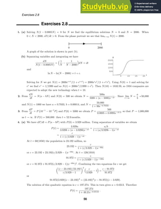
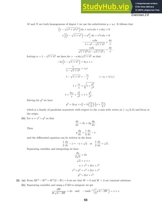
Exercises 2.8
from part (a) and solve for t. This gives the time of extinction
t = −
1
3
ln
4(P0 − 1)
P0 − 4
.
6. (a) Solving P(5 − P) − 25
4 = 0 for P we obtain the equilibrium solution P = 5
2 . For P = 5
2 , dP/dt 0. Thus,
if P0 5
2 , the population becomes extinct (otherwise there would be another equilibrium solution.) Using
separation of variables to solve the initial-value problem we get P(t) = [4P0 +(10P0 −25)t]/[4+(4P0 −10)t].
To find when the population becomes extinct for P0 5
2 we solve P(t) = 0 for t. We see that the time of
extinction is t = 4P0/5(5 − 2P0).
(b) Solving P(5 − P) − 7 = 0 for P we obtain complex roots, so there are no equilibrium solutions. Since
dP/dt 0 for all values of P, the population becomes extinct for any initial condition. Using separation of
variables to solve the initial-value problem we get
P(t) =
5
2
+
√
3
2
tan
tan−1
2P0 − 5
√
3
−
√
3
2
t
.
Solving P(t) = 0 for t we see that the time of extinction is
t =
2
3
√
3 tan−1
(5/
√
3 ) +
√
3 tan−1
(2P0 − 5)/
√
3
.
7. (a) The differential equation is dP/dt = P(1 − ln P), which has equilibrium solution
P = e. When P0 e, dP/dt 0, and when P0 e, dP/dt 0.
(b) The differential equation is dP/dt = P(1 + ln P), which has equilibrium solution
P = 1/e. When P0 1/e, dP/dt 0, and when Po 1/e, dP/dt 0.
(c) From
dP
dt
= P(a − b ln P) we obtain
−1
b
ln |a − b ln P| = t + c1 so that P = ea/b
e−ce−bt
. If P(0) = P0 then
c =
a
b
− ln P0.
8. (a) Using a CAS to solve P(1 − P) + 0.3e−P
= 0 for P we see that P = 1.09216 is an equilibrium solution.
(b) Since f(P) 0 for 0 P 1.09216, the solution P(t) of
dP/dt = P(1 − P) + 0.3e−P
, P(0) = P0,
is increasing for P0 1.09216. Since f(P) 0 for P 1.09216, the solution
P(t) is decreasing for P0 1.09216. Thus P = 1.09216 is an attractor.
58](https://image.slidesharecdn.com/advancedengineeringmathematicssolutionsmanual-230807162553-1916df96/85/Advanced-Engineering-Mathematics-Solutions-Manual-pdf-58-320.jpg)


![Exercises 2.9
5. The system is
x
1 = 2 · 3 +
1
50
x2 −
1
50
x1 · 4 = −
2
25
x1 +
1
50
x2 + 6
x
2 =
1
50
x1 · 4 −
1
50
x2 −
1
50
x2 · 3 =
2
25
x1 −
2
25
x2.
6. Let x1, x2, and x3 be the amounts of salt in tanks A, B, and C, respectively, so that
x
1 =
1
100
x2 · 2 −
1
100
x1 · 6 =
1
50
x2 −
3
50
x1
x
2 =
1
100
x1 · 6 +
1
100
x3 −
1
100
x2 · 2 −
1
100
x2 · 5 =
3
50
x1 −
7
100
x2 +
1
100
x3
x
3 =
1
100
x2 · 5 −
1
100
x3 −
1
100
x3 · 4 =
1
20
x2 −
1
20
x3.
7. (a) A model is
dx1
dt
= 3 ·
x2
100 − t
− 2 ·
x1
100 + t
, x1(0) = 100
dx2
dt
= 2 ·
x1
100 + t
− 3 ·
x2
100 − t
, x2(0) = 50.
(b) Since the system is closed, no salt enters or leaves the system and x1(t) + x2(t) = 100 + 50 = 150 for all
time. Thus x1 = 150 − x2 and the second equation in part (a) becomes
dx2
dt
=
2(150 − x2)
100 + t
−
3x2
100 − t
=
300
100 + t
−
2x2
100 + t
−
3x2
100 − t
or
dx2
dt
+
2
100 + t
+
3
100 − t
x2 =
300
100 + t
,
which is linear in x2. An integrating factor is
e2 ln(100+t)−3 ln(100−t)
= (100 + t)2
(100 − t)−3
so
d
dt
[(100 + t)2
(100 − t)−3
x2] = 300(100 + t)(100 − t)−3
.
Using integration by parts, we obtain
(100 + t)2
(100 − t)−3
x2 = 300
1
2
(100 + t)(100 − t)−2
−
1
2
(100 − t)−1
+ c
.
Thus
x2 =
300
(100 + t)2
c(100 − t)3
−
1
2
(100 − t)2
+
1
2
(100 + t)(100 − t)
=
300
(100 + t)2
[c(100 − t)3
+ t(100 − t)].
Using x2(0) = 50 we find c = 5/3000. At t = 30, x2 = (300/1302
)(703
c + 30 · 70) ≈ 47.4lbs.
8. A model is
dx1
dt
= (4 gal/min)(0 lb/gal) − (4 gal/min)
1
200
x1 lb/gal
dx2
dt
= (4 gal/min)
1
200
x1 lb/gal
− (4 gal/min)
1
150
x2 lb/gal
dx3
dt
= (4 gal/min)
1
150
x2 lb/gal
− (4 gal/min)
1
100
x3 lb/gal
67](https://image.slidesharecdn.com/advancedengineeringmathematicssolutionsmanual-230807162553-1916df96/85/Advanced-Engineering-Mathematics-Solutions-Manual-pdf-67-320.jpg)

![Chapter 2 Review Exercises
10. Write the differential equation in the form y ln
x
y
dx =
x ln
x
y
− y
dy. This is a homogeneous equation, so let
x = uy. Then dx = u dy + y du and the differential equation becomes
y ln u(u dy + y du) = (uy ln u − y) dy or y ln u du = −dy.
Separating variables we obtain
ln u du = −
dy
y
=⇒ u ln |u| − u = − ln |y| + c =⇒
x
y
ln
x
y
−
x
y
= − ln |y| + c
=⇒ x(ln x − ln y) − x = −y ln |y| + cy.
11. The differential equation
dy
dx
+
2
6x + 1
y = −
3x2
6x + 1
y−2
is Bernoulli. Using w = y3
we obtain
dw
dx
+
6
6x + 1
w =
−
9x2
6x + 1
. An integrating factor is 6x + 1, so
d
dx
[(6x + 1)w] = −9x2
=⇒ w = −
3x3
6x + 1
+
c
6x + 1
=⇒ (6x + 1)y3
= −3x3
+ c.
(Note: The differential equation is also exact.)
12. Write the differential equation in the form (3y2
+ 2x)dx + (4y2
+ 6xy)dy = 0. Letting M = 3y2
+ 2x and
N = 4y2
+ 6xy we see that My = 6y = Nx so the differential equation is exact. From fx = 3y2
+ 2x we obtain
f = 3xy2
+ x2
+ h(y). Then fy = 6xy + h
(y) = 4y2
+ 6xy and h
(y) = 4y2
so h(y) = 4
3 y3
. The general solution
is
3xy2
+ x2
+
4
3
y3
= c.
13. Write the equation in the form
dQ
dt
+
1
t
Q = t3
ln t.
An integrating factor is eln t
= t, so
d
dt
[tQ] = t4
ln t =⇒ tQ = −
1
25
t5
+
1
5
t5
ln t + c
=⇒ Q = −
1
25
t4
+
1
5
t4
ln t +
c
t
.
14. Letting u = 2x + y + 1 we have
du
dx
= 2 +
dy
dx
,
and so the given differential equation is transformed into
u
du
dx
− 2
= 1 or
du
dx
=
2u + 1
u
.
Separating variables and integrating we get
u
2u + 1
du = dx
1
2
−
1
2
1
2u + 1
du = dx
1
2
u −
1
4
ln |2u + 1| = x + c
2u − ln |2u + 1| = 2x + c1.
72](https://image.slidesharecdn.com/advancedengineeringmathematicssolutionsmanual-230807162553-1916df96/85/Advanced-Engineering-Mathematics-Solutions-Manual-pdf-72-320.jpg)
![t
y
Chapter 2 Review Exercises
Resubstituting for u gives the solution
4x + 2y + 2 − ln |4x + 2y + 3| = 2x + c1
or
2x + 2y + 2 − ln |4x + 2y + 3| = c1.
15. Write the equation in the form
dy
dx
+
8x
x2 + 4
y =
2x
x2 + 4
. An integrating factor is
x2
+ 4
4
, so
d
dx
x2
+ 4
4
y
= 2x
x2
+ 4
3
=⇒
x2
+ 4
4
y =
1
4
x2
+ 4
4
+ c =⇒ y =
1
4
+ c
x2
+ 4
−4
.
16. Letting M = 2r2
cos θ sin θ + r cos θ and N = 4r + sin θ − 2r cos2
θ we see that Mr = 4r cos θ sin θ + cos θ = Nθ
so the differential equation is exact. From fθ = 2r2
cos θ sin θ + r cos θ we obtain f = −r2
cos2
θ + r sin θ + h(r).
Then fr = −2r cos2
θ + sin θ + h
(r) = 4r + sin θ − 2r cos2
θ and h
(r) = 4r so h(r) = 2r2
. The general solution
is
−r2
cos2
θ + r sin θ + 2r2
= c.
17. The differential equation has the form
d
dx
[(sin x)y] = 0. Integrating we have (sin x)y = c or
y = c/ sin x. The initial condition implies c = −2 sin(7π/6) = 1. Thus, y = 1/ sin x, where π x 2π is
chosen to include x = 7π/6.
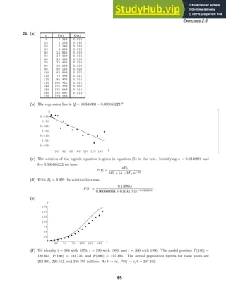
18. For y t the slopes are negative and for y t the slopes are positive, so the
differential equation is (a).
19. (a) For y 0,
√
y is not a real number.
(b) Separating variables and integrating we have
dy
√
y
= dx and 2
√
y = x + c.
Letting y(x0) = y0 we get c = 2
√
y0 − x0, so that
2
√
y = x + 2
√
y0 − x0 and y =
1
4
(x + 2
√
y0 − x0)2
.
Since
√
y 0 for y = 0, we see that dy/dx = 1
2 (x + 2
√
y0 − x0) must be positive. Thus, the interval on
which the solution is defined is (x0 − 2
√
y0, ∞).
73](https://image.slidesharecdn.com/advancedengineeringmathematicssolutionsmanual-230807162553-1916df96/85/Advanced-Engineering-Mathematics-Solutions-Manual-pdf-73-320.jpg)
![-2 -1 1 2 x
-2
-1
1
2
y
Chapter 2 Review Exercises
20. (a) The differential equation is homogeneous and we let y = ux. Then
(x2
− y2
) dx + xy dy = 0
(x2
− u2
x2
) dx + ux2
(u dx + x du) = 0
dx + ux du = 0
u du = −
dx
x
1
2
u2
= − ln |x| + c
y2
x2
= −2 ln |x| + c1.
The initial condition gives c1 = 2, so an implicit solution is y2
= x2
(2 − 2 ln |x|).
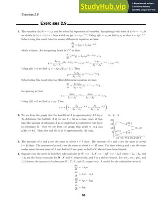
(b) Solving for y in part (a) and being sure that the initial condition is still satisfied, we have y =
−
√
2 |x|(1 − ln |x|)1/2
, where −e ≤ x ≤ e so that 1 − ln |x| ≥ 0. A graph of this function shown be-
low indicates that the derivative is not defined at x = 0 and x = e. Thus, the solution of the initial-value
problem is y = −
√
2 x(1 − ln x)1/2
, for 0 x e.
21. The graph of y1(x) is the portion of the closed black curve lying in the fourth quadrant. Its interval of definition
is approximately (0.7, 4.3). The graph of y2(x) is the portion of the left-hand black curve lying in the third
quadrant. Its interval of definition is (−∞, 0).
22. The first step of Euler’s method gives y(1.1) ≈ 9 + 0.1(1 + 3) = 9.4. Applying Euler’s method one more time
gives y(1.2) ≈ 9.4 + 0.1(1 + 1.1
√
9.4 ) ≈ 9.8373.
23. From
dP
dt
= 0.018P and P(0) = 4 billion we obtain P = 4e0.018t
so that P(45) = 8.99 billion.
24. Let A = A(t) be the volume of CO2 at time t. From
dA
dt
= 1.2 −
A
4
and A(0) = 16 ft3
we obtain A =
4.8 + 11.2e−t/4
. Since A(10) = 5.7 ft3
, the concentration is 0.017%. As t → ∞ we have A → 4.8 ft3
or 0.06%.
25. From dE/dt = −E/RC and E(t1) = E0 we obtain E = E0e(t1−t)/RC
.
26. From V dC/dt = kA(Cs − C) and C(0) = C0 we obtain C = Cs + (C0 − Cs)e−kAt/V
.
27. (a) The differential equation is
dT
dt
= k[T − T2 − B(T1 − T)] = k[(1 + B)T − (BT1 + T2)].
Separating variables we obtain
dT
(1 + B)T − (BT1 + T2)
= k dt. Then
1
1 + B
ln |(1 + B)T − (BT1 + T2)| = kt + c and T(t) =
BT1 + T2
1 + B
+ c3ek(1+B)t
.
Since T(0) = T1 we must have c3 =
T1 − T2
1 + B
and so
T(t) =
BT1 + T2
1 + B
+
T1 − T2
1 + B
ek(1+B)t
.
74](https://image.slidesharecdn.com/advancedengineeringmathematicssolutionsmanual-230807162553-1916df96/85/Advanced-Engineering-Mathematics-Solutions-Manual-pdf-74-320.jpg)
![10 20
10
20
x
y
-5 5
-5
5
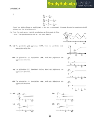
Chapter 2 Review Exercises
(b) Since k 0, lim
t→∞
ek(1+B)t
= 0 and lim
t→∞
T(t) =
BT1 + T2
1 + B
.
(c) Since Ts = T2 + B(T1 − T), lim
t→∞
Ts = T2 + BT1 − B
BT1 + T2
1 + B
=
BT1 + T2
1 + B
.
28. We first solve
1 −
t
10
di
dt
+ 0.2i = 4. Separating variables we obtain
di
40 − 2i
=
dt
10 − t
.
Then
−
1
2
ln |40 − 2i| = − ln |10 − t| + c or
√
40 − 2i = c1(10 − t).
Since i(0) = 0 we must have c1 = 2/
√
10 . Solving for i we get i(t) = 4t − 1
5 t2
,
0 ≤ t 10. For t ≥ 10 the equation for the current becomes 0.2i = 4 or i = 20. Thus
i(t) =
4t − 1
5 t2
, 0 ≤ t 10
20, t ≥ 10
.
29. From y 1 + (y
)2
= k we obtain dx =
√
y
√
k − y
dy. If y = k sin2
θ then
dy = 2k sin θ cos θ dθ, dx = 2k
1
2
−
1
2
cos 2θ
dθ, and x = kθ −
k
2
sin 2θ + c.
If x = 0 when θ = 0 then c = 0.
30. (a) From y = −x − 1 + c1ex
we obtain y
= y + x so that the differential equation of the orthogonal family is
dy
dx
= −
1
y + x
or
dx
dy
+ x = −y. An integrating factor is ey
, so
d
dy
[ey
x] = −yey
=⇒ ey
x = −yey
+ ey
+ c =⇒ x = −y + 1 + ce−y
.
(b) Differentiating the family of curves, we have
y
= −
1
(x + c1)2
= −
1
y2
.
The differential equation for the family of orthogonal trajectories is then
y
= y2
. Separating variables and integrating we get
dy
y2
= dx
−
1
y
= x + c1
y = −
1
x + c1
.
31. From
dx
dt
= k1x(α − x) we obtain
1/α
x
+
1/α
α − x
dx = k1 dt so that x =
αc1eαk1t
1 + c1eαk1t
. From
dy
dt
= k2xy we
obtain
ln |y| =
k2
k1
ln 1 + c1eαk1t
+ c or y = c2
1 + c1eαk1t k2/k1
.
75](https://image.slidesharecdn.com/advancedengineeringmathematicssolutionsmanual-230807162553-1916df96/85/Advanced-Engineering-Mathematics-Solutions-Manual-pdf-75-320.jpg)

![Exercises 3.2
Exercises 3.2
In Problems 1-8 we use reduction of order to find a second solution. In Problems 9-16 we use formula (5) from the
text.
1. Define y = u(x)e2x
so
y
= 2ue2x
+ u
e2x
, y
= e2x
u
+ 4e2x
u
+ 4e2x
u, and y
− 4y
+ 4y = 4e2x
u
= 0.
Therefore u
= 0 and u = c1x + c2. Taking c1 = 1 and c2 = 0 we see that a second solution is y2 = xe2x
.
2. Define y = u(x)xe−x
so
y
= (1 − x)e−x
u + xe−x
u
, y
= xe−x
u
+ 2(1 − x)e−x
u
− (2 − x)e−x
u,
and
y
+ 2y
+ y = e−x
(xu
+ 2u
) = 0 or u
+
2
x
u
= 0.
If w = u
we obtain the first-order equation w
+
2
x
w = 0 which has the integrating factor e2
dx/x
= x2
. Now
d
dx
[x2
w] = 0 gives x2
w = c.
Therefore w = u
= c/x2
and u = c1/x. A second solution is y2 =
1
x
xe−x
= e−x
.
3. Define y = u(x) cos 4x so
y
= −4u sin 4x + u
cos 4x, y
= u
cos 4x − 8u
sin 4x − 16u cos 4x
and
y
+ 16y = (cos 4x)u
− 8(sin 4x)u
= 0 or u
− 8(tan 4x)u
= 0.
If w = u
we obtain the first-order equation w
−8(tan 4x)w = 0 which has the integrating factor e−8
tan 4x dx
=
cos2
4x. Now
d
dx
[(cos2
4x)w] = 0 gives (cos2
4x)w = c.
Therefore w = u
= c sec2
4x and u = c1 tan 4x. A second solution is y2 = tan 4x cos 4x = sin 4x.
4. Define y = u(x) sin 3x so
y
= 3u cos 3x + u
sin 3x, y
= u
sin 3x + 6u
cos 3x − 9u sin 3x,
and
y
+ 9y = (sin 3x)u
+ 6(cos 3x)u
= 0 or u
+ 6(cot 3x)u
= 0.
If w = u
we obtain the first-order equation w
+ 6(cot 3x)w = 0 which has the integrating factor e6
cot 3x dx
=
sin2
3x. Now
d
dx
[(sin2
3x)w] = 0 gives (sin2
3x)w = c.
Therefore w = u
= c csc2
3x and u = c1 cot 3x. A second solution is y2 = cot 3x sin 3x = cos 3x.
5. Define y = u(x) cosh x so
y
= u sinh x + u
cosh x, y
= u
cosh x + 2u
sinh x + u cosh x
and
y
− y = (cosh x)u
+ 2(sinh x)u
= 0 or u
+ 2(tanh x)u
= 0.
81](https://image.slidesharecdn.com/advancedengineeringmathematicssolutionsmanual-230807162553-1916df96/85/Advanced-Engineering-Mathematics-Solutions-Manual-pdf-81-320.jpg)
![Exercises 3.2
If w = u
we obtain the first-order equation w
+ 2(tanh x)w = 0 which has the integrating factor e2
tanh x dx
=
cosh2
x. Now
d
dx
[(cosh2
x)w] = 0 gives (cosh2
x)w = c.
Therefore w = u
= c sech2
x and u = c1 tanh x. A second solution is y2 = tanh x cosh x = sinh x.
6. Define y = u(x)e5x
so
y
= 5e5x
u + e5x
u
, y
= e5x
u
+ 10e5x
u
+ 25e5x
u
and
y
− 25y = e5x
(u
+ 10u
) = 0 or u
+ 10u
= 0.
If w = u
we obtain the first-order equation w
+ 10w = 0 which has the integrating factor e10
dx
= e10x
. Now
d
dx
[e10x
w] = 0 gives e10x
w = c.
Therefore w = u
= ce−10x
and u = c1e−10x
. A second solution is y2 = e−10x
e5x
= e−5x
.
7. Define y = u(x)e2x/3
so
y
=
2
3
e2x/3
u + e2x/3
u
, y
= e2x/3
u
+
4
3
e2x/3
u
+
4
9
e2x/3
u
and
9y
− 12y
+ 4y = 9e2x/3
u
= 0.
Therefore u
= 0 and u = c1x + c2. Taking c1 = 1 and c2 = 0 we see that a second solution is y2 = xe2x/3
.
8. Define y = u(x)ex/3
so
y
=
1
3
ex/3
u + ex/3
u
, y
= ex/3
u
+
2
3
ex/3
u
+
1
9
ex/3
u
and
6y
+ y
− y = ex/3
(6u
+ 5u
) = 0 or u
+
5
6
u
= 0.
If w = u
we obtain the first-order equation w
+ 5
6 w = 0 which has the integrating factor e(5/6)
dx
= e5x/6
.
Now
d
dx
[e5x/6
w] = 0 gives e5x/6
w = c.
Therefore w = u
= ce−5x/6
and u = c1e−5x/6
. A second solution is y2 = e−5x/6
ex/3
= e−x/2
.
9. Identifying P(x) = −7/x we have
y2 = x4
e−
−(7/x) dx
x8
dx = x4
1
x
dx = x4
ln |x|.
A second solution is y2 = x4
ln |x|.
10. Identifying P(x) = 2/x we have
y2 = x2
e−
(2/x) dx
x4
dx = x2
x−6
dx = −
1
5
x−3
.
A second solution is y2 = x−3
.
11. Identifying P(x) = 1/x we have
y2 = ln x
e−
dx/x
(ln x)2
dx = ln x
dx
x(ln x)2
= ln x −
1
ln x
= −1.
82](https://image.slidesharecdn.com/advancedengineeringmathematicssolutionsmanual-230807162553-1916df96/85/Advanced-Engineering-Mathematics-Solutions-Manual-pdf-82-320.jpg)
![Exercises 3.2
A second solution is y2 = 1.
12. Identifying P(x) = 0 we have
y2 = x1/2
ln x
e−
0 dx
x(ln x)2
= x1/2
ln x −
1
ln x
= −x1/2
.
A second solution is y2 = x1/2
.
13. Identifying P(x) = −1/x we have
y2 = x sin(ln x)
e−
−dx/x
x2 sin2
(ln x)
dx = x sin(ln x)
x
x2 sin2
(ln x)
dx
= [x sin(ln x)] [− cot(ln x)] = −x cos(ln x).
A second solution is y2 = x cos(ln x).
14. Identifying P(x) = −3/x we have
y2 = x2
cos(ln x)
e−
−3 dx/x
x4 cos2(ln x)
dx = x2
cos(ln x)
x3
x4 cos2(ln x)
dx
= x2
cos(ln x) tan(ln x) = x2
sin(ln x).
A second solution is y2 = x2
sin(ln x).
15. Identifying P(x) = 2(1 + x)/
1 − 2x − x2
we have
y2 = (x + 1)
e−
2(1+x)dx/(1−2x−x2
)
(x + 1)2
dx = (x + 1)
eln(1−2x−x2
)
(x + 1)2
dx
= (x + 1)
1 − 2x − x2
(x + 1)2
dx = (x + 1)
2
(x + 1)2
− 1 dx
= (x + 1) −
2
x + 1
− x = −2 − x2
− x.
A second solution is y2 = x2
+ x + 2.
16. Identifying P(x) = −2x/
1 − x2
we have
y2 =
e−
−2x dx/(1−x2
)dx =
e− ln(1−x2
)dx =
1
1 − x2
dx =
1
2
ln
1 + x
1 − x
.
A second solution is y2 = ln |(1 + x)/(1 − x)|.
17. Define y = u(x)e−2x
so
y
= −2ue−2x
+ u
e−2x
, y
= u
e−2x
− 4u
e−2x
+ 4ue−2x
and
y
− 4y = e−2x
u
− 4e−2x
u
= 0 or u
− 4u
= 0.
If w = u
we obtain the first order equation w
− 4w = 0 which has the integrating factor e−4
dx
= e−4x
. Now
d
dx
[e−4x
w] = 0 gives e−4x
w = c.
Therefore w = u
= ce4x
and u = c1e4x
. A second solution is y2 = e−2x
e4x
= e2x
. We see by observation that a
particular solution is yp = −1/2. The general solution is
y = c1e−2x
+ c2e2x
−
1
2
.
83](https://image.slidesharecdn.com/advancedengineeringmathematicssolutionsmanual-230807162553-1916df96/85/Advanced-Engineering-Mathematics-Solutions-Manual-pdf-83-320.jpg)
![Exercises 3.2
18. Define y = u(x) · 1 so
y
= u
, y
= u
and y
+ y
= u
+ u
= 0.
If w = u
we obtain the first order equation w
+ w = 0 which has the integrating factor e
dx
= ex
. Now
d
dx
[ex
w] = 0 gives ex
w = c.
Therefore w = u
= ce−x
and u = c1e−x
. A second solution is y2 = 1 · e−x
= e−x
. We see by observation that
a particular solution is yp = x. The general solution is
y = c1 + c2e−x
+ x.
19. Define y = u(x)ex
so
y
= uex
+ u
ex
, y
= u
ex
+ 2u
ex
+ uex
and
y
− 3y
+ 2y = ex
u
− ex
u
= 0 or u
− u
= 0.
If w = u
we obtain the first order equation w
− w = 0 which has the integrating factor e−
dx
= e−x
. Now
d
dx
[e−x
w] = 0 gives e−x
w = c.
Therefore w = u
= cex
and u = cex
. A second solution is y2 = ex
ex
= e2x
. To find a particular solution we
try yp = Ae3x
. Then y
= 3Ae3x
, y
= 9Ae3x
, and 9Ae3x
− 3
3Ae3x
+ 2Ae3x
= 5e3x
. Thus A = 5/2 and
yp = 5
2 e3x
. The general solution is
y = c1ex
+ c2e2x
+
5
2
e3x
.
20. Define y = u(x)ex
so
y
= uex
+ u
ex
, y
= u
ex
+ 2u
ex
+ uex
and
y
− 4y
+ 3y = ex
u
− 2ex
u
= 0 or u
− 2u
= 0.
If w = u
we obtain the first order equation w
− 2w = 0 which has the integrating factor e−2
dx
= e−2x
. Now
d
dx
[e−2x
w] = 0 gives e−2x
w = c.
Therefore w = u
= ce2x
and u = c1e2x
. A second solution is y2 = ex
e2x
= e3x
. To find a particular solution
we try yp = ax + b. Then y
p = a, y
p = 0, and 0 − 4a + 3(ax + b) = 3ax − 4a + 3b = x. Then 3a = 1 and
−4a + 3b = 0 so a = 1/3 and b = 4/9. A particular solution is yp = 1
3 x + 4
9 and the general solution is
y = c1ex
+ c2e3x
+
1
3
x +
4
9
.
21. (a) For m1 constant, let y1 = em1x
. Then y
1 = m1em1x
and y
1 = m2
1em1x
. Substituting into the differential
equation we obtain
ay
1 + by
1 + cy1 = am2
1em1x
+ bm1em1x
+ cem1x
= em1x
(am2
1 + bm1 + c) = 0.
Thus, y1 = em1x
will be a solution of the differential equation whenever am2
1+bm1+c = 0. Since a quadratic
equation always has at least one real or complex root, the differential equation must have a solution of the
form y1 = em1x
.
(b) Write the differential equation in the form
y
+
b
a
y
+
c
a
y = 0,
84](https://image.slidesharecdn.com/advancedengineeringmathematicssolutionsmanual-230807162553-1916df96/85/Advanced-Engineering-Mathematics-Solutions-Manual-pdf-84-320.jpg)
![Exercises 3.3
m2 = 0.658675, and m3 = 5.61186. The general solution is
y = c1e−0.270534x
+ c2e0.658675x
+ c3e5.61186x
.
46. Using a CAS to solve the auxiliary equation 6.11m3
+ 8.59m2
+ 7.93m + 0.778 = 0 we find
m1 = −0.110241, m2 = −0.647826 + 0.857532i, and m3 = −0.647826 − 0.857532i. The general solution is
y = c1e−0.110241x
+ e−0.647826x
(c2 cos 0.857532x + c3 sin 0.857532x).
47. Using a CAS to solve the auxiliary equation 3.15m4
− 5.34m2
+ 6.33m − 2.03 = 0 we find
m1 = −1.74806, m2 = 0.501219, m3 = 0.62342+0.588965i, and m4 = 0.62342−0.588965i. The general solution
is
y = c1e−1.74806x
+ c2e0.501219x
+ e0.62342x
(c3 cos 0.588965x + c4 sin 0.588965x).
48. Using a CAS to solve the auxiliary equation m4
+2m2
−m+2 = 0 we find m1 = 1/2+
√
3 i/2, m2 = 1/2−
√
3 i/2,
m3 = −1/2 +
√
7 i/2, and m4 = −1/2 −
√
7 i/2. The general solution is
y = ex/2
c1 cos
√
3
2
x + c2 sin
√
3
2
x
+ e−x/2
c3 cos
√
7
2
x + c4 sin
√
7
2
x
.
49. The auxiliary equation should have two positive roots, so that the solution has the form y = c1ek1x
+ c2ek2x
.
Thus, the differential equation is (f).
50. The auxiliary equation should have one positive and one negative root, so that the solution has the form
y = c1ek1x
+ c2e−k2x
. Thus, the differential equation is (a).
51. The auxiliary equation should have a pair of complex roots a ± bi where a 0, so that the solution has the
form eax
(c1 cos bx + c2 sin bx). Thus, the differential equation is (e).
52. The auxiliary equation should have a repeated negative root, so that the solution has the form y = c1e−x
+
c2xe−x
. Thus, the differential equation is (c).
53. The differential equation should have the form y
+ k2
y = 0 where k = 1 so that the period of the solution is
2π. Thus, the differential equation is (d).
54. The differential equation should have the form y
+ k2
y = 0 where k = 2 so that the period of the solution is
π. Thus, the differential equation is (b).
55. (a) The auxiliary equation is m2
− 64/L = 0 which has roots ±8/
√
L . Thus, the general solution of the
differential equation is x = c1 cosh(8t/
√
L ) + c2 sinh(8t/
√
L ).
(b) Setting x(0) = x0 and x
(0) = 0 we have c1 = x0, 8c2/
√
L = 0. Solving for c1 and c2 we get c1 = x0 and
c2 = 0, so x(t) = x0 cosh(8t/
√
L ).
(c) When L = 20 and x0 = 1, x(t) = cosh(4t
√
5 ). The chain will last touch the peg when x(t) = 10.
Solving x(t) = 10 for t we get t1 = 1
4
√
5 cosh−1
10 ≈ 1.67326. The velocity of the chain at this instant is
x
(t1) = 12
11/5 ≈ 17.7989 ft/s.
56. Both −C[1] and c1 represent arbitrary constants, and each may take on any real value.
57. Since (m − 4)(m + 5)2
= m3
+ 6m2
− 15m − 100 the differential equation is y
+ 6y
− 15y
− 100y = 0. The
differential equation is not unique since any constant multiple of the left-hand side of the differential equation
would lead to the auxiliary roots.
58. A third root must be m3 = 3 − i and the auxiliary equation is
m +
1
2
[m − (3 + i)][m − (3 − i)] =
m +
1
2
(m2
− 6x + 10) = m3
−
11
2
m2
+ 7m + 5.
89](https://image.slidesharecdn.com/advancedengineeringmathematicssolutionsmanual-230807162553-1916df96/85/Advanced-Engineering-Mathematics-Solutions-Manual-pdf-89-320.jpg)


![Exercises 3.4
37. We have yc = c1 cos x + c2 sin x and we assume yp = A2
+ Bx + C. Substituting into the differential equation
we find A = 1, B = 0, and C = −1. Thus y = c1 cos x + c2 sin x + x2
− 1. From y(0) = 5 and y(1) = 0 we obtain
c1 − 1 = 5
(cos 1)c1 + sin(1)c2 = 0.
Solving this system we find c1 = 6 and c2 = −6 cot 1. The solution of the boundary-value problem is
y = 6 cos x − 6(cot 1) sin x + x2
− 1.
38. We have yc = ex
(c1 cos x + c2 sin x) and we assume yp = Ax + B. Substituting into the differential equation we
find A = 1 and B = 0. Thus y = ex
(c1 cos x + c2 sin x) + x. From y(0) = 0 and y(π) = π we obtain
c1 = 0
π − eπ
c1 = π.
Solving this system we find c1 = 0 and c2 is any real number. The solution of the boundary-value problem is
y = c2ex
sin x + x.
39. We have yc = c1 cos 2x + c2 sin 2x and we assume yp = A cos x + B sin x on [0, π/2]. Substituting into the
differential equation we find A = 0 and B = 1
3 . Thus y = c1 cos 2x + c2 sin 2x + 1
3 sin x on [0, π/2]. On (π/2, ∞)
we have y = c3 cos 2x + c4 sin 2x. From y(0) = 1 and y
(0) = 2 we obtain
c1 = 1
1
3
+ 2c2 = 2.
Solving this system we find c1 = 1 and c2 = 5
6 . Thus y = cos 2x + 5
6 sin 2x + 1
3 sin x on [0, π/2]. Now continuity
of y at x = π/2 implies
cos π +
5
6
sin π +
1
3
sin
π
2
= c3 cos π + c4 sin π
or −1 + 1
3 = −c3. Hence c3 = 2
3 . Continuity of y
at x = π/2 implies
−2 sin π +
5
3
cos π +
1
3
cos
π
2
= −2c3 sin π + 2c4 cos π
or −5
3 = −2c4. Then c4 = 5
6 and the solution of the boundary-value problem is
y(x) =
cos 2x + 5
6 sin 2x + 1
3 sin x, 0 ≤ x ≤ π/2
2
3 cos 2x + 5
6 sin 2x, x π/2.
40. The complementary function is yc = e2x
(c1 cos 2x + c2 sin 2x). We assume a particular solution of the form
yp = (Ax3
+ Bx2
+ Cx)e2x
cos 2x + (Dx3
+ Ex2
+ F)e2x
sin 2x. Substituting into the differential equation and
using a CAS to simplify yields
[12Dx2
+ (6A + 8E)x + (2B + 4F)]e2x
cos 2x + [−12Ax2
+ (−8B + 6D)x + (−4C + 2E)]e2x
sin 2x
= (2x2
− 3x)e2x
cos 2x + (10x2
− x − 1)e2x
sin 2x.
This gives the system of equations
12D = 2,
−12A = 10,
6A + 8E = −3,
−8B + 6D = −1,
2B + 4F = 0,
−4C + 2E = −1,
96](https://image.slidesharecdn.com/advancedengineeringmathematicssolutionsmanual-230807162553-1916df96/85/Advanced-Engineering-Mathematics-Solutions-Manual-pdf-96-320.jpg)
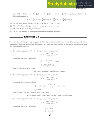


![Exercises 3.6
The general solution is
y = c1x2
+
c2
x2
−
1
16x2
−
1
4x2
ln x.
Exercises 3.6
1. The auxiliary equation is m2
− m − 2 = (m + 1)(m − 2) = 0 so that y = c1x−1
+ c2x2
.
2. The auxiliary equation is 4m2
− 4m + 1 = (2m − 1)2
= 0 so that y = c1x1/2
+ c2x1/2
ln x.
3. The auxiliary equation is m2
= 0 so that y = c1 + c2 ln x.
4. The auxiliary equation is m2
− 4m = m(m − 4) = 0 so that y = c1 + c2x4
.
5. The auxiliary equation is m2
+ 4 = 0 so that y = c1 cos(2 ln x) + c2 sin(2 ln x).
6. The auxiliary equation is m2
+ 4m + 3 = (m + 1)(m + 3) = 0 so that y = c1x−1
+ c2x−3
.
7. The auxiliary equation is m2
− 4m − 2 = 0 so that y = c1x2−
√
6
+ c2x2+
√
6
.
8. The auxiliary equation is m2
+ 2m − 4 = 0 so that y = c1x−1+
√
5
+ c2x−1−
√
5
.
9. The auxiliary equation is 25m2
+ 1 = 0 so that y = c1 cos
1
5 ln x
+ c2
1
5 ln x
.
10. The auxiliary equation is 4m2
− 1 = (2m − 1)(2m + 1) = 0 so that y = c1x1/2
+ c2x−1/2
.
11. The auxiliary equation is m2
+ 4m + 4 = (m + 2)2
= 0 so that y = c1x−2
+ c2x−2
ln x.
12. The auxiliary equation is m2
+ 7m + 6 = (m + 1)(m + 6) = 0 so that y = c1x−1
+ c2x−6
.
13. The auxiliary equation is 3m2
+ 3m + 1 = 0 so that y = x−1/2
c1 cos
√
3
6 ln x
+ c2 sin
√
3
6 ln x
.
14. The auxiliary equation is m2
− 8m + 41 = 0 so that y = x4
[c1 cos(5 ln x) + c2 sin(5 ln x)].
15. Assuming that y = xm
and substituting into the differential equation we obtain
m(m − 1)(m − 2) − 6 = m3
− 3m2
+ 2m − 6 = (m − 3)(m2
+ 2) = 0.
Thus
y = c1x3
+ c2 cos
√
2 ln x
+ c3 sin
√
2 ln x
.
16. Assuming that y = xm
and substituting into the differential equation we obtain
m(m − 1)(m − 2) + m − 1 = m3
− 3m2
+ 3m − 1 = (m − 1)3
= 0.
Thus
y = c1x + c2x ln x + c3x(ln x)2
.
17. Assuming that y = xm
and substituting into the differential equation we obtain
m(m − 1)(m − 2)(m − 3) + 6m(m − 1)(m − 2) = m4
− 7m2
+ 6m = m(m − 1)(m − 2)(m + 3) = 0.
Thus
y = c1 + c2x + c3x2
+ c4x−3
.
18. Assuming that y = xm
and substituting into the differential equation we obtain
m(m − 1)(m − 2)(m − 3) + 6m(m − 1)(m − 2) + 9m(m − 1) + 3m + 1 = m4
+ 2m2
+ 1 = (m2
+ 1)2
= 0.
Thus
y = c1 cos(ln x) + c2 sin(ln x) + c3 ln x cos(ln x) + c4 ln x sin(ln x).
109](https://image.slidesharecdn.com/advancedengineeringmathematicssolutionsmanual-230807162553-1916df96/85/Advanced-Engineering-Mathematics-Solutions-Manual-pdf-109-320.jpg)


![Exercises 3.6
The auxiliary equation is m2
−4m+13 = 0 so that yc = e2t
(c1 cos 3t+c2 sin 3t). Using undetermined coefficients
we try yp = A + Bet
. This leads to 13A + 10Bet
= 4 + 3et
, so that A = 4/13, B = 3/10, and
y = e2t
(c1 cos 3t + c2 sin 3t) +
4
13
+
3
10
et
= x2
[c1 cos(3 ln x) + c2 sin(3 ln x)] +
4
13
+
3
10
x.
32. From
d2
y
dx2
=
1
x2
d2
y
dt2
−
dy
dt
it follows that
d3
y
dx3
=
1
x2
d
dx
d2
y
dt2
−
dy
dt
−
2
x3
d2
y
dt2
−
dy
dt
=
1
x2
d
dx
d2
y
dt2
−
1
x2
d
dx
dy
dt
−
2
x3
d2
y
dt2
+
2
x3
dy
dt
=
1
x2
d3
y
dt3
1
x
−
1
x2
d2
y
dt2
1
x
−
2
x3
d2
y
dt2
+
2
x3
dy
dt
=
1
x3
d3
y
dt3
− 3
d2
y
dt2
+ 2
dy
dt
.
Substituting into the differential equation we obtain
d3
y
dt3
− 3
d2
y
dt2
+ 2
dy
dt
− 3
d2
y
dt2
−
dy
dt
+ 6
dy
dt
− 6y = 3 + 3t
or
d3
y
dt3
− 6
d2
y
dt2
+ 11
dy
dt
− 6y = 3 + 3t.
The auxiliary equation is m3
−6m2
+11m−6 = (m−1)(m−2)(m−3) = 0 so that yc = c1et
+c2e2t
+c3e3t
. Using
undetermined coefficients we try yp = A + Bt. This leads to (11B − 6A) − 6Bt = 3 + 3t, so that A = −17/12,
B = −1/2, and
y = c1et
+ c2e2t
+ c3e3t
−
17
12
−
1
2
t = c1x + c2x2
+ c3x3
−
17
12
−
1
2
ln x.
33. The auxiliary equation is 2m(m − 1)(m − 2) − 10.98m(m − 1) + 8.5m + 1.3 = 0, so that m1 = −0.053299,
m2 = 1.81164, m3 = 6.73166, and
y = c1x−0.053299
+ c2x1.81164
+ c3x6.73166
.
34. The auxiliary equation is m(m − 1)(m − 2) + 4m(m − 1) + 5m − 9 = 0, so that m1 = 1.40819 and the two
complex roots are −1.20409 ± 2.22291i. The general solution of the differential equation is
y = c1x1.40819
+ x−1.20409
[c2 cos(2.22291 ln x) + c3 sin(2.22291 ln x)].
35. The auxiliary equation is m(m − 1)(m − 2)(m − 3) + 6m(m − 1)(m − 2) + 3m(m − 1) − 3m + 4 = 0, so that
m1 = m2 =
√
2 and m3 = m4 = −
√
2 . The general solution of the differential equation is
y = c1x
√
2
+ c2x
√
2
ln x + c3x−
√
2
+ c4x−
√
2
ln x.
36. The auxiliary equation is m(m − 1)(m − 2)(m − 3) − 6m(m − 1)(m − 2) + 33m(m − 1) − 105m + 169 = 0, so
that m1 = m2 = 3 + 2i and m3 = m4 = 3 − 2i. The general solution of the differential equation is
y = x3
[c1 cos(2 ln x) + c2 sin(2 ln x)] + x3
ln x[c3 cos(2 ln x) + c4 sin(2 ln x)].
112](https://image.slidesharecdn.com/advancedengineeringmathematicssolutionsmanual-230807162553-1916df96/85/Advanced-Engineering-Mathematics-Solutions-Manual-pdf-112-320.jpg)
![Exercises 3.6
In the next two problems we use the substitution t = −x since the initial conditions are on the interval (−∞, 0). In
this case
dy
dt
=
dy
dx
dx
dt
= −
dy
dx
and
d2
y
dt2
=
d
dt
dy
dt
=
d
dt
−
dy
dx
= −
d
dt
(y
) = −
dy
dx
dx
dt
= −
d2
y
dx2
dx
dt
=
d2
y
dx2
.
37. The differential equation and initial conditions become
4t2 d2
y
dt2
+ y = 0; y(t)
t=1
= 2, y
(t)
t=1
= −4.
The auxiliary equation is 4m2
− 4m + 1 = (2m − 1)2
= 0, so that
y = c1t1/2
+ c2t1/2
ln t and y
=
1
2
c1t−1/2
+ c2 t−1/2
+
1
2
t−1/2
ln t .
The initial conditions imply c1 = 2 and 1 + c2 = −4. Thus
y = 2t1/2
− 5t1/2
ln t = 2(−x)1/2
− 5(−x)1/2
ln(−x), x 0.
38. The differential equation and initial conditions become
t2 d2
y
dt2
− 4t
dy
dt
+ 6y = 0; y(t)
t=2
= 8, y
(t)
t=2
= 0.
The auxiliary equation is m2
− 5m + 6 = (m − 2)(m − 3) = 0, so that
y = c1t2
+ c2t3
and y
= 2c1t + 3c2t2
.
The initial conditions imply
4c1 + 8c2 = 8
4c1 + 12c2 = 0
from which we find c1 = 6 and c2 = −2. Thus
y = 6t2
− 2t3
= 6x2
+ 2x3
, x 0.
39. Letting u = x + 2 we obtain
dy
dx
=
dy
du
and, using the chain rule,
d2
y
dx2
=
d
dx
dy
du
=
d2
y
du2
du
dx
=
d2
y
du2
(1) =
d2
y
du2
.
Substituting into the differential equation we obtain
u2 d2
y
du2
+ u
dy
du
+ y = 0.
The auxiliary equation is m2
+ 1 = 0 so that
y = c1 cos(ln u) + c2 sin(ln u) = c1 cos[ ln(x + 2)] + c2 sin[ ln(x + 2)].
40. If 1 − i is a root of the auxiliary equation then so is 1 + i, and the auxiliary equation is
(m − 2)[m − (1 + i)][m − (1 − i)] = m3
− 4m2
+ 6m − 4 = 0.
113](https://image.slidesharecdn.com/advancedengineeringmathematicssolutionsmanual-230807162553-1916df96/85/Advanced-Engineering-Mathematics-Solutions-Manual-pdf-113-320.jpg)
![Exercises 3.6
We need m3
− 4m2
+ 6m − 4 to have the form m(m − 1)(m − 2) + bm(m − 1) + cm + d. Expanding this last
expression and equating coefficients we get b = −1, c = 3, and d = −4. Thus, the differential equation is
x3
y
− x2
y
+ 3xy
− 4y = 0.
41. For x2
y
= 0 the auxiliary equation is m(m − 1) = 0 and the general solution is y = c1 + c2x. The initial
conditions imply c1 = y0 and c2 = y1, so y = y0 + y1x. The initial conditions are satisfied for all real values of
y0 and y1.
For x2
y
− 2xy
+ 2y = 0 the auxiliary equation is m2
− 3m + 2 = (m − 1)(m − 2) = 0 and the general solution
is y = c1x + c2x2
. The initial condition y(0) = y0 implies 0 = y0 and the condition y
(0) = y1 implies c1 = y1.
Thus, the initial conditions are satisfied for y0 = 0 and for all real values of y1.
For x2
y
− 4xy
+ 6y = 0 the auxiliary equation is m2
− 5m + 6 = (m − 2)(m − 3) = 0 and the general solution
is y = c1x2
+ c2x3
. The initial conditions imply y(0) = 0 = y0 and y
(0) = 0. Thus, the initial conditions are
satisfied only for y0 = y1 = 0.
42. The function y(x) = −
√
x cos(ln x) is defined for x 0 and has x-intercepts where ln x = π/2 + kπ for k an
integer or where x = eπ/2+kπ
. Solving π/2 + kπ = 0.5 we get k ≈ −0.34, so eπ/2+kπ
0.5 for all negative
integers and the graph has infinitely many x-intercepts in (0, 0.5).
Exercises 3.7
1. We have y
1 = y
1 = ex
, so
(y
1 )2
= (ex
)2
= e2x
= y2
1.
Also, y
2 = − sin x and y
2 = − cos x, so
(y
2 )2
= (− cos x)2
= cos2
x = y2
2.
However, if y = c1y1 + c2y2, we have (y
)2
= (c1ex
− c2 cos x)2
and y2
= (c1ex
+ c2 cos x)2
. Thus (y
)2
= y2
.
2. We have y
1 = y
1 = 0, so
y1y
1 = 1 · 0 = 0 =
1
2
(0)2
=
1
2
(y
1)2
.
Also, y
2 = 2x and y
2 = 2, so
y2y
2 = x2
(2) = 2x2
=
1
2
(2x)2
=
1
2
(y
2)2
.
However, if y = c1y1 + c2y2, we have yy
= (c1 · 1 + c2x2
)(c1 · 0 + 2c2) = 2c2(c1 + c2x2
) and 1
2 (y
)2
=
1
2 [c1 · 0 + c2(2x)]2
= 2c2
2x2
. Thus yy
= 1
2 (y
)2
.
3. Let u = y
so that u
= y
. The equation becomes u
= −u − 1 which is separable. Thus
du
u2 + 1
= −dx =⇒ tan−1
u = −x + c1 =⇒ y
= tan(c1 − x) =⇒ y = ln | cos(c1 − x)| + c2.
4. Let u = y
so that u
= y
. The equation becomes u
= 1 + u2
. Separating variables we obtain
du
1 + u2
= dx =⇒ tan−1
u = x + c1 =⇒ u = tan(x + c1) =⇒ y = − ln | cos(x + c1)| + c2.
114](https://image.slidesharecdn.com/advancedengineeringmathematicssolutionsmanual-230807162553-1916df96/85/Advanced-Engineering-Mathematics-Solutions-Manual-pdf-114-320.jpg)

![x
y
2
−2π 2π
x
y
−1
1
−2π 2π
Exercises 3.7
10. Let u = y
so that u
= y
. The equation becomes (u
)2
+ u2
= 1
which results in u
= ±
√
1 − u2 . To solve u
=
√
1 − u2 we separate
variables:
du
√
1 − u2
= dx =⇒ sin−1
u = x + c1 =⇒ u = sin(x + c1)
=⇒ y
= sin(x + c1).
When x =
π
2
, y
=
√
3
2
, so
√
3
2
= sin
π
2
+ c1
and c1 = −
π
6
. Thus
y
= sin
x −
π
6
=⇒ y = − cos
x −
π
6
+ c2.
When x =
π
2
, y =
1
2
, so
1
2
= − cos
π
2
−
π
6
+ c2 = −
1
2
+ c2 and c2 = 1. The solution of the initial-value
problem is y = 1 − cos
x −
π
6
.
To solve u
= −
√
1 − u2 we separate variables:
du
√
1 − u2
= −dx =⇒ cos−1
u = x + c1
=⇒ u = cos(x + c1) =⇒ y
= cos(x + c1).
When x =
π
2
, y
=
√
3
2
, so
√
3
2
= cos
π
2
+ c1
and c1 = −
π
3
. Thus
y
= cos
x −
π
3
=⇒ y = sin
x −
π
3
+ c2.
When x =
π
2
, y =
1
2
, so
1
2
= sin
π
2
−
π
3
+ c2 =
1
2
+ c2 and c2 = 0. The solution of the initial-value
problem is y = sin
x −
π
3
.
11. Let u = y
so that u
= y
. The equation becomes u
−
1
x
u =
1
x
u3
, which is Bernoulli. Using w = u−2
we obtain
dw
dx
+
2
x
w = −
2
x
. An integrating factor is x2
, so
d
dx
[x2
w] = −2x =⇒ x2
w = −x2
+ c1 =⇒ w = −1 +
c1
x2
=⇒ u−2
= −1 +
c1
x2
=⇒ u =
x
√
c1 − x2
=⇒
dy
dx
=
x
√
c1 − x2
=⇒ y = −
c1 − x2 + c2
=⇒ c1 − x2
= (c2 − y)2
=⇒ x2
+ (c2 − y)2
= c1.
12. Let u = y
so that u
= y
. The equation becomes u
−
1
x
u = u2
, which is Bernoulli. Using the substitution
w = u−1
we obtain
dw
dx
+
1
x
w = −1. An integrating factor is x, so
d
dx
[xw] = −x =⇒ w = −
1
2
x +
1
x
c =⇒
1
u
=
c1 − x2
2x
=⇒ u =
2x
c1 − x2
=⇒ y = − ln
c1 − x2
+ c2.
116](https://image.slidesharecdn.com/advancedengineeringmathematicssolutionsmanual-230807162553-1916df96/85/Advanced-Engineering-Mathematics-Solutions-Manual-pdf-116-320.jpg)


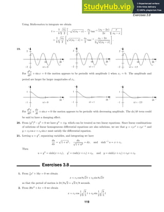

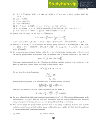
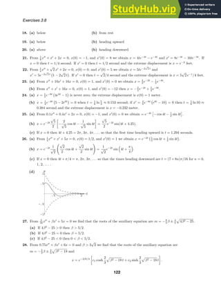
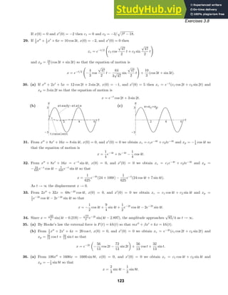
![1 2 3 t
-1
1
x
t
x
−1
1
π 9π
Exercises 3.8
(b) If x = 1
3 sin 4t(2 − 2 cos 4t) = 0 then t = nπ/4 for n = 0, 1, 2, . . . .
(c) If x
= 8
3 cos 4t − 8
3 cos 8t = 8
3 (1 − cos 4t)(1 + 2 cos 4t) = 0 then t = π/3 + nπ/2 and t = π/6 + nπ/2 for
n = 0, 1, 2, . . . at the extreme values. Note: There are many other values of t for which x
= 0.
(d) x(π/6 + nπ/2) =
√
3/2 cm. and x(π/3 + nπ/2) = −
√
3/2 cm.
(e)
37. From x
+ 4x = −5 sin 2t + 3 cos 2t, x(0) = −1, and x
(0) = 1 we obtain xc = c1 cos 2t + c2 sin 2t,
xp = 3
4 t sin 2t + 5
4 t cos 2t, and
x = − cos 2t −
1
8
sin 2t +
3
4
t sin 2t +
5
4
t cos 2t.
38. From x
+ 9x = 5 sin 3t, x(0) = 2, and x
(0) = 0 we obtain xc = c1 cos 3t + c2 sin 3t, xp = −5
6 t cos 3t, and
x = 2 cos 3t +
5
18
sin 3t −
5
6
t cos 3t.
39. (a) From x
+ ω2
x = F0 cos γt, x(0) = 0, and x
(0) = 0 we obtain xc = c1 cos ωt + c2 sin ωt and
xp = (F0 cos γt)/
ω2
− γ2
so that
x = −
F0
ω2 − γ2
cos ωt +
F0
ω2 − γ2
cos γt.
(b) lim
γ→ω
F0
ω2 − γ2
(cos γt − cos ωt) = lim
γ→ω
−F0t sin γt
−2γ
=
F0
2ω
t sin ωt.
40. From x
+ω2
x = F0 cos ωt, x(0) = 0, and x
(0) = 0 we obtain xc = c1 cos ωt+c2 sin ωt and xp = (F0t/2ω) sin ωt
so that x = (F0t/2ω) sin ωt and lim
γ→ω
F0
2ω
t sin ωt =
F0
2ω
t sin ωt.
41. (a) From cos(u − v) = cos u cos v + sin u sin v and cos(u + v) = cos u cos v − sin u sin v we obtain sin u sin v =
1
2 [cos(u − v) − cos(u + v)]. Letting u = 1
2 (γ − ω)t and v = 1
2 (γ + ω)t, the result follows.
(b) If + = 1
2 (γ − ω) then γ ≈ ω so that x = (F0/2+γ) sin +t sin γt.
42. See the article ”Distinguished Oscillations of a Forced Harmonic Oscillator” by T.G. Procter in The College
Mathematics Journal, March, 1995. In this article the author illustrates that for F0 = 1, λ = 0.01, γ = 22/9,
and ω = 2 the system exhibits beats oscillations on the interval [0, 9π], but that this phenomenon is transient
as t → ∞.
124](https://image.slidesharecdn.com/advancedengineeringmathematicssolutionsmanual-230807162553-1916df96/85/Advanced-Engineering-Mathematics-Solutions-Manual-pdf-124-320.jpg)
![β γ1 g
2.00 1.41 0.58
1.00 1.87 1.03
0.75 1.93 1.36
0.50 1.97 2.02
0.25 1.99 4.01
1 2 3 4
γ
1
2
3
4
g
β=0.25
β=0.5
β=0.75
β=1
β=2
Exercises 3.8
43. (a) The general solution of the homogeneous equation is
xc(t) = c1e−λt
cos(
ω2 − λ2 t) + c2e−λt
sin(
ω2 − λ2 t)
= Ae−λt
sin[
ω2 − λ2 t + φ],
where A =
c2
1 + c2
2 , sin φ = c1/A, and cos φ = c2/A. Now
xp(t) =
F0(ω2
− γ2
)
(ω2 − γ2)2 + 4λ2γ2
sin γt +
F0(−2λγ)
(ω2 − γ2)2 + 4λ2γ2
cos γt = A sin(γt + θ),
where
sin θ =
F0(−2λγ)
(ω2 − γ2)2 + 4λ2γ2
F0
ω2 − γ2 + 4λ2
γ2
=
−2λγ
(ω2 − γ2)2 + 4λ2γ2
and
cos θ =
F0(ω2
− γ2
)
(ω2 − γ2)2 + 4λ2γ2
F0
(ω2 − γ2)2 + 4λ2γ2
=
ω2
− γ2
(ω2 − γ2)2 + 4λ2γ2
.
(b) If g
(γ) = 0 then γ
γ2
+ 2λ2
− ω2
= 0 so that γ = 0 or γ =
√
ω2 − 2λ2. The first derivative test shows
that g has a maximum value at γ =
√
ω2 − 2λ2 . The maximum value of g is
g
ω2 − 2λ2
= F0/2λ
ω2 − λ2.
(c) We identify ω2
= k/m = 4, λ = β/2, and γ1 =
√
ω2 − 2λ2 =
4 − β2/2 . As β → 0, γ1 → 2 and the
resonance curve grows without bound at γ1 = 2. That is, the system approaches pure resonance.
44. (a) For n = 2, sin2
γt = 1
2 (1 − cos 2γt). The system is in pure resonance when 2γ1/2π = ω/2π, or when
γ1 = ω/2.
(b) Note that
sin3
γt = sin γt sin2
γt =
1
2
[sin γt − sin γt cos 2γt].
Now
sin(A + B) + sin(A − B) = 2 sin A cos B
125](https://image.slidesharecdn.com/advancedengineeringmathematicssolutionsmanual-230807162553-1916df96/85/Advanced-Engineering-Mathematics-Solutions-Manual-pdf-125-320.jpg)
![10 20 30
t
γ1=1/2
-10
-5
5
10
x
n=2
10 20 30
t
γ1=1
-10
-5
5
10
x
n=3
20 40
t
γ2=1/3
-10
-5
5
10
x
n=3
Exercises 3.8
so
sin γt cos 2γt =
1
2
[sin 3γt − sin γt]
and
sin3
γt =
3
4
sin γt −
1
4
sin 3γt.
Thus
x
+ ω2
x =
3
4
sin γt −
1
4
sin 3γt.
The frequency of free vibration is ω/2π. Thus, when γ1/2π = ω/2π or γ1 = ω, and when 3γ2/2π = ω/2π
or 3γ2 = ω or γ3 = ω/3, the system will be in pure resonance.
(c)
45. Solving 1
20 q
+ 2q
+ 100q = 0 we obtain q(t) = e−20t
(c1 cos 40t + c2 sin 40t). The initial conditions q(0) = 5 and
q
(0) = 0 imply c1 = 5 and c2 = 5/2. Thus
q(t) = e−20t
5 cos 40t +
5
2
sin 40t ≈
25 + 25/4 e−20t
sin(40t + 1.1071)
and q(0.01) ≈ 4.5676 coulombs. The charge is zero for the first time when 40t + 0.4636 = π or t ≈ 0.0509
second.
46. Solving 1
4 q
+ 20q
+ 300q = 0 we obtain q(t) = c1e−20t
+ c2e−60t
. The initial conditions q(0) = 4 and q
(0) = 0
imply c1 = 6 and c2 = −2. Thus
q(t) = 6e−20t
− 2e−60t
.
Setting q = 0 we find e40t
= 1/3 which implies t 0. Therefore the charge is never 0.
47. Solving 5
3 q
+ 10q
+ 30q = 300 we obtain q(t) = e−3t
(c1 cos 3t + c2 sin 3t) + 10. The initial conditions q(0) =
q
(0) = 0 imply c1 = c2 = −10. Thus
q(t) = 10 − 10e−3t
(cos 3t + sin 3t) and i(t) = 60e3t
sin 3t.
Solving i(t) = 0 we see that the maximum charge occurs when t = π/3 and q(π/3) ≈ 10.432 coulombs.
48. Solving q
+ 100q
+ 2500q = 30 we obtain q(t) = c1e−50t
+ c2te−50t
+ 0.012. The initial conditions q(0) = 0
and q
(0) = 2 imply c1 = −0.012 and c2 = 1.4. Thus
q(t) = −0.012e−50t
+ 1.4te−50t
+ 0.012 and i(t) = 2e−50t
− 70te−50t
.
Solving i(t) = 0 we see that the maximum charge occurs when t = 1/35 and q(1/35) ≈ 0.01871.
49. Solving q
+ 2q
+ 4q = 0 we obtain yc = e−t
cos
√
3 t + sin
√
3 t
. The steady-state charge has the form
yp = A cos t + B sin t. Substituting into the differential equation we find
(3A + 2B) cos t + (3B − 2A) sin t = 50 cos t.
Thus, A = 150/13 and B = 100/13. The steady-state charge is
qp(t) =
150
13
cos t +
100
13
sin t
126](https://image.slidesharecdn.com/advancedengineeringmathematicssolutionsmanual-230807162553-1916df96/85/Advanced-Engineering-Mathematics-Solutions-Manual-pdf-126-320.jpg)
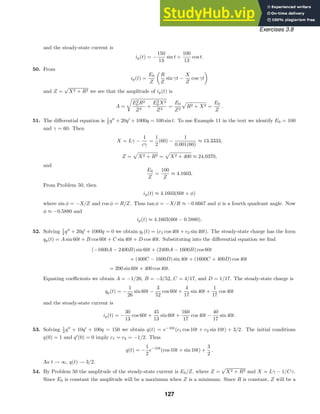

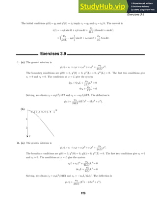
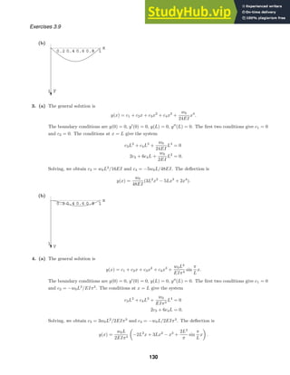
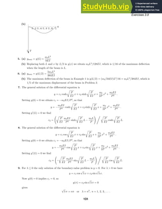

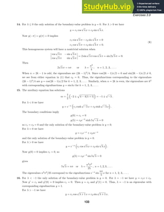
![Exercises 3.9
Now
y
= −c1
√
λ + 1 sin
√
λ + 1 x + c2
√
λ + 1 cos
√
λ + 1 x
and y
(0) = 0 implies c2 = 0, so
y
(1) = −c1
√
λ + 1 sin
√
λ + 1 = 0
gives
√
λ + 1 = nπ or λ = n2
π2
− 1, n = 1, 2, 3, . . . .
The eigenvalues n2
π2
− 1 correspond to the eigenfunctions cos nπx for n = 0, 1, 2, . . . .
17. For λ = 0 the only solution of the boundary-value problem is y = 0. For λ = 0 we have
y = c1 cos λx + c2 sin λx.
Now y(0) = 0 implies c1 = 0, so
y(L) = c2 sin λL = 0
gives
λL = nπ or λ =
nπ
L
, n = 1, 2, 3, . . . .
The eigenvalues nπ/L correspond to the eigenfunctions sin
nπ
L
x for n = 1, 2, 3, . . . .
18. For λ = 0 the only solution of the boundary-value problem is y = 0. For λ = 0 we have
y = c1 cos λx + c2 sin λx.
Now y(0) = 0 implies c1 = 0, so
y
(3π) = c2λ cos 3πλ = 0
gives
3πλ =
(2n − 1)π
2
or λ =
2n − 1
6
, n = 1, 2, 3, . . . .
The eigenvalues (2n − 1)/6 correspond to the eigenfunctions sin
2n − 1
6
x for n = 1, 2, 3, . . . .
19. For λ 0 a general solution of the given differential equation is
y = c1 cos(
√
λ ln x) + c2 sin(
√
λ ln x).
Since ln 1 = 0, the boundary condition y(1) = 0 implies c1 = 0. Therefore
y = c2 sin(
√
λ ln x).
Using ln eπ
= π we find that y (eπ
) = 0 implies
c2 sin
√
λ π = 0
or
√
λ π = nπ, n = 1, 2, 3, . . . . The eigenvalues and eigenfunctions are, in turn,
λ = n2
, n = 1, 2, 3, . . . and y = sin(n ln x).
For λ ≤ 0 the only solution of the boundary-value problem is y = 0.
To obtain the self-adjoint form we note that the integrating factor is (1/x2
)e
dx/x
= 1/x. That is, the self-
adjoint form is
d
dx
[xy
] +
λ
x
y = 0.
134](https://image.slidesharecdn.com/advancedengineeringmathematicssolutionsmanual-230807162553-1916df96/85/Advanced-Engineering-Mathematics-Solutions-Manual-pdf-134-320.jpg)

![Exercises 3.9
Thus
u(r) =
u0 − u1
b − a
ab
r
+
u1b − u0a
b − a
.
30. The auxiliary equation is m2
= 0 so that u(r) = c1 + c2 ln r. The boundary conditions u(a) = u0 and u(b) = u1
yield the system c1 + c2 ln a = u0, c1 + c2 ln b = u1. Solving gives
c1 =
u1 ln a − u0 ln b
ln(a/b)
and c2 =
u0 − u1
ln(a/b)
.
Thus
u(r) =
u1 ln a − u0 ln b
ln(a/b)
+
u0 − u1
ln(a/b)
ln r =
u0 ln(r/b) − u1 ln(r/a)
ln(a/b)
.
31. (a) The general solution of the differential equation is y = c1 cos 4x + c2 sin 4x. From y0 = y(0) = c1 we see
that y = y0 cos 4x + c2 sin 4x. From y1 = y(π/2) = y0 we see that any solution must satisfy y0 = y1. We
also see that when y0 = y1, y = y0 cos 4x + c2 sin 4x is a solution of the boundary-value problem for any
choice of c2. Thus, the boundary-value problem does not have a unique solution for any choice of y0 and
y1.
(b) Whenever y0 = y1 there are infinitely many solutions.
(c) When y0 = y1 there will be no solutions.
(d) The boundary-value problem will have the trivial solution when y0 = y1 = 0. This solution will not be
unique.
32. (a) The general solution of the differential equation is y = c1 cos 4x + c2 sin 4x. From 1 = y(0) = c1 we see that
y = cos 4x + c2 sin 4x. From 1 = y(L) = cos 4L + c2 sin 4L we see that c2 = (1 − cos 4L)/ sin 4L. Thus,
y = cos 4x +
1 − cos 4L
sin 4L
sin 4x
will be a unique solution when sin 4L = 0; that is, when L = kπ/4 where k = 1, 2, 3, . . . .
(b) There will be infinitely many solutions when sin 4L = 0 and 1 − cos 4L = 0; that is, when L = kπ/2 where
k = 1, 2, 3, . . . .
(c) There will be no solution when sin 4L = 0 and 1 − cos 4L = 0; that is, when L = kπ/4 where
k = 1, 3, 5, . . . .
(d) There can be no trivial solution since it would fail to satisfy the boundary conditions.
33. (a) A solution curve has the same y-coordinate at both ends of the interval [−π, π] and the tangent lines at the
endpoints of the interval are parallel.
(b) For λ = 0 the solution of y
= 0 is y = c1x + c2. From the first boundary condition we have
y(−π) = −c1π + c2 = y(π) = c1π + c2
or 2c1π = 0. Thus, c1 = 0 and y = c2. This constant solution is seen to satisfy the boundary-value problem.
For λ 0 we have y = c1 cosh λx + c2 sinh λx. In this case the first boundary condition gives
y(−π) = c1 cosh(−λπ) + c2 sinh(−λπ)
= c1 cosh λπ − c2 sinh λπ
= y(π) = c1 cosh λπ + c2 sinh λπ
or 2c2 sinh λπ = 0. Thus c2 = 0 and y = c1 cosh λx. The second boundary condition implies in a similar
fashion that c1 = 0. Thus, for λ 0, the only solution of the boundary-value problem is y = 0.
138](https://image.slidesharecdn.com/advancedengineeringmathematicssolutionsmanual-230807162553-1916df96/85/Advanced-Engineering-Mathematics-Solutions-Manual-pdf-138-320.jpg)
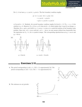
![2 4 6 8 10
t
2
4
6
8
10
-2
x
2 4 6 8 10
t
1
2
3
-1
-2
-3
x
x1=1.1
x1=1.2
t
x
5 10
−1
1
2
3
4
t
x
5 10
−1
1
2
3
Exercises 3.10
3. The period corresponding to x(0) = 1, x
(0) = 1 is approximately 5.8.
The second initial-value problem does not have a periodic solution.
4. Both solutions have periods of approximately 6.3.
5. From the graph we see that |x1| ≈ 1.2.
6. From the graphs we see that the interval is approximately (−0.8, 1.1).
7. Since
xe0.01x
= x[1 + 0.01x +
1
2!
(0.01x)2
+ · · · ] ≈ x
for small values of x, a linearization is
d2
x
dt2
+ x = 0.
140](https://image.slidesharecdn.com/advancedengineeringmathematicssolutionsmanual-230807162553-1916df96/85/Advanced-Engineering-Mathematics-Solutions-Manual-pdf-140-320.jpg)
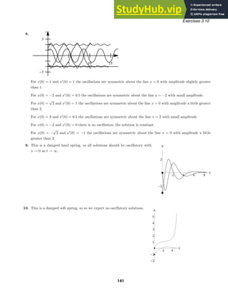
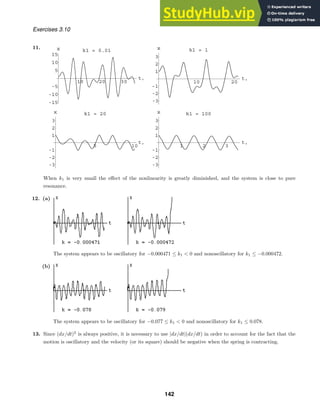

![1 2 3 4 5
-0.4
-0.2
0.2
0.4
2 4 6 8 10
-0.4
-0.2
0.2
0.4
Exercises 3.10
16. (a) The general solution of
d2
θ
dt2
+ θ = 0
is θ(t) = c1 cos t + c2 sin t. From θ(0) = π/12 and θ
(0) = −1/3 we find θ(t) = (π/12) cos t − (1/3) sin t.
Setting θ(t) = 0 we have tan t = π/4 which implies t1 = tan−1
(π/4) ≈ 0.66577.
(b) We set θ(t) = θ(0) + θ
(0)t + 1
2 θ
(0)t + 1
6 θ
(0)t + · · · and use θ
(t) = − sin θ(t) together with
θ(0) = π/12 and θ
(0) = −1/3. Then θ
(0) = − sin(π/12) = −
√
2 (
√
3−1)/4 and θ
(0) = − cos θ(0)·θ
(0) =
− cos(π/12)(−1/3) =
√
2 (
√
3 + 1)/12. Thus
θ(t) =
π
12
−
1
3
t −
√
2 (
√
3 − 1)
8
t2
+
√
2 (
√
3 + 1)
72
t3
+ · · · .
(c) Setting π/12 − t/3 = 0 we obtain t1 = π/4 ≈ 0.785398.
(d) Setting
π
12
−
1
3
t −
√
2 (
√
3 − 1)
8
t2
= 0
and using the positive root we obtain t1 ≈ 0.63088.
(e) Setting
π
12
−
1
3
t −
√
2 (
√
3 − 1)
8
t2
+
√
2 (
√
3 + 1)
72
t3
= 0
we find t1 ≈ 0.661973 to be the first positive root.
(f) From the output we see that y(t) is an interpolating function on the interval
0 ≤ t ≤ 5, whose graph is shown. The positive root of y(t) = 0 near t = 1
is t1 = 0.666404.
(g) To find the next two positive roots we change the interval used in NDSolve
and Plot from {t,0,5} to {t,0,10}. We see from the graph that the second
and third positive roots are near 4 and 7, respectively. Replacing {t,1}
in FindRoot with {t,4} and then {t,7} we obtain t2 = 3.84411 and
t3 = 7.0218.
17. From the table below we see that the pendulum first passes the vertical position between 1.7 and 1.8 seconds.
To refine our estimate of t1 we estimate the solution of the differential equation on [1.7, 1.8] using a step size of
h = 0.01. From the resulting table we see that t1 is between 1.76 and 1.77 seconds. Repeating the process with
h = 0.001 we conclude that t1 ≈ 1.767. Then the period of the pendulum is approximately 4t1 = 7.068. The
error when using t1 = 2π is 7.068 − 6.283 = 0.785 and the percentage relative error is (0.785/7.068)100 = 11.1.
144](https://image.slidesharecdn.com/advancedengineeringmathematicssolutionsmanual-230807162553-1916df96/85/Advanced-Engineering-Mathematics-Solutions-Manual-pdf-144-320.jpg)
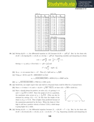
![Exercises 3.10
obtain
v
v2 + Lg
dv =
1
L − x
dx and
1
2
ln(v2
+ Lg) = − ln(L − x) + ln c,
so
v2 + Lg = c/(L − x). When x = 0, v = 0, and c = L
√
Lg . Solving for v and simplifying we get
dx
dt
= v(x) =
Lg(2Lx − x2)
L − x
.
Again, separating variables and integrating we obtain
L − x
Lg(2Lx − x2)
dx = dt and
√
2Lx − x2
√
Lg
= t + c1.
Since x(0) = 0, we have c1 = 0 and
√
2Lx − x2/
√
Lg = t. Solving for x we get
x(t) = L −
L2 − Lgt2 and v(t) =
dx
dt
=
√
Lgt
L − gt2
.
(b) The chain will be completely on the ground when x(t) = L or t =
L/g .
(c) The predicted velocity of the upper end of the chain when it hits the ground is infinity.
21. (a) The weight of x feet of the chain is 2x, so the corresponding mass is m = 2x/32 = x/16. The only force
acting on the chain is the weight of the portion of the chain hanging over the edge of the platform. Thus,
by Newton’s second law,
d
dt
(mv) =
d
dt
x
16
v =
1
16
x
dv
dt
+ v
dx
dt
=
1
16
x
dv
dt
+ v2
= 2x
and x dv/dt+v2
= 32x. Now, by the chain rule, dv/dt = (dv/dx)(dx/dt) = v dv/dx, so xv dv/dx+v2
= 32x.
(b) We separate variables and write the differential equation as (v2
− 32x) dx + xv dv = 0. This is not an exact
form, but µ(x) = x is an integrating factor. Multiplying by x we get (xv2
− 32x2
) dx + x2
v dv = 0. This
form is the total differential of u = 1
2 x2
v2
− 32
3 x3
, so an implicit solution is 1
2 x2
v2
− 32
3 x3
= c. Letting x = 3
and v = 0 we find c = −288. Solving for v we get
dx
dt
= v =
8
√
x3 − 27
√
3x
, 3 ≤ x ≤ 8.
(c) Separating variables and integrating we obtain
x
√
x3 − 27
dx =
8
√
3
dt and
x
3
s
√
s3 − 27
ds =
8
√
3
t + c.
Since x = 3 when t = 0, we see that c = 0 and
t =
√
3
8
x
3
s
√
s3 − 27
ds.
We want to find t when x = 7. Using a CAS we find t(7) = 0.576 seconds.
22. (a) There are two forces acting on the chain as it falls from the platform. One is the force due to gravity on
the portion of the chain hanging over the edge of the platform. This is F1 = 2x. The second is due to the
motion of the portion of the chain stretched out on the platform. By Newton’s second law this is
F2 =
d
dt
[mv] =
d
dt
(8 − x)2
32
v =
d
dt
8 − x
16
v
=
8 − x
16
dv
dt
−
1
16
v
dx
dt
=
1
16
(8 − x)
dv
dt
− v2
.
146](https://image.slidesharecdn.com/advancedengineeringmathematicssolutionsmanual-230807162553-1916df96/85/Advanced-Engineering-Mathematics-Solutions-Manual-pdf-146-320.jpg)
![Exercises 3.10
From
d
dt
[mv] = F1 − F2 we have
d
dt
2x
32
v = 2x −
1
16
(8 − x)
dv
dt
− v2
x
16
dv
dt
+
1
16
v
dx
dt
= 2x −
1
16
(8 − x)
dv
dt
− v2
x
dv
dt
+ v2
= 32x − (8 − x)
dv
dt
+ v2
x
dv
dt
= 32x − 8
dv
dt
+ x
dv
dt
8
dv
dt
= 32x.
By the chain rule, dv/dt = (dv/dx)(dx/dt) = v dv/dx, so
8
dv
dt
= 8v
dv
dx
= 32x and v
dv
dx
= 4x.
(b) Integrating v dv = 4x dx we get 1
2 v2
= 2x2
+ c. Since v = 0 when x = 3, we have c = −18. Then
v2
= 4x2
− 36 and v =
√
4x2 − 36 . Using v = dx/dt, separating variables, and integrating we obtain
dx
√
x2 − 9
= 2 dt and cosh−1 x
3
= 2t + c1.
Solving for x we get x(t) = 3 cosh(2t + c1). Since x = 3 when t = 0, we have cosh c1 = 1 and c1 = 0. Thus,
x(t) = 3 cosh 2t. Differentiating, we find v(t) = dx/dt = 6 sinh 2t.
(c) To find when the back end of the chain will leave the platform we solve x(t) = 3 cosh 2t = 8. This gives t1 =
1
2 cosh−1 8
3 ≈ 0.8184 seconds. The velocity at this instant is v(t1) = 6 sinh
cosh−1 8
3
= 2
√
55 ≈ 14.83 ft/s.
(d) Replacing 8 with L and 32 with g in part (a) we have L dv/dt = gx. Then
L
dv
dt
= Lv
dv
dx
= gx and v
dv
dx
=
g
L
x.
Integrating we get
1
2
v2
=
g
2L
x2
+ c. Setting x = x0 and v = 0, we find c = −
g
2L
x2
0. Solving for v we find
v(x) =
g
L
x2 −
g
L
x2
0 .
Then the velocity at which the end of the chain leaves the edge of the platform is
v(L) =
g
L
(L2 − x2
0) .
23. (a) Let (x, y) be the coordinates of S2 on the curve C. The slope at (x, y) is then
dy/dx = (v1t − y)/(0 − x) = (y − v1t)/x or xy
− y = −v1t.
(b) Differentiating with respect to x gives
xy
+ y
− y
= −v1
dt
dx
xy
= −v1
dt
ds
ds
dx
xy
= −v1
1
v2
(−
1 + (y)2 )
xy
= r
1 + (y)2 .
147](https://image.slidesharecdn.com/advancedengineeringmathematicssolutionsmanual-230807162553-1916df96/85/Advanced-Engineering-Mathematics-Solutions-Manual-pdf-147-320.jpg)
![Exercises 3.10
Letting u = y
and separating variables, we obtain
x
du
dx
= r
1 + u2
du
√
1 + u2
=
r
x
dx
sinh−1
u = r ln x + ln c = ln(cxr
)
u = sinh(ln cxr
)
dy
dx
=
1
2
cxr
−
1
cxr
.
At t = 0, dy/dx = 0 and x = a, so 0 = car
− 1/car
. Thus c = 1/ar
and
dy
dx
=
1
2
x
a
r
−
a
x
r
=
1
2
x
a
r
−
x
a
−r
.
If r 1 or r 1, integrating gives
y =
a
2
1
1 + r
x
a
1+r
−
1
1 − r
x
a
1−r
+ c1.
When t = 0, y = 0 and x = a, so 0 = (a/2)[1/(1 + r) − 1/(1 − r)] + c1. Thus c1 = ar/(1 − r2
) and
y =
a
2
1
1 + r
x
a
1+r
−
1
1 − r
x
a
1−r
+
ar
1 − r2
.
(c) If r 1, v1 v2 and y → ∞ as x → 0+
. In other words, S2 always lags behind S1. If r 1, v1 v2 and
y = ar/(1 − r2
) when x = 0. In other words, when the submarine’s speed is greater than the ship’s, their
paths will intersect at the point (0, ar/(1 − r2
)).
If r = 1, integration gives
y =
1
2
x2
2a
−
1
a
ln x + c2.
When t = 0, y = 0 and x = a, so 0 = (1/2)[a/2 − (1/a) ln a] + c2. Thus c2 = −(1/2)[a/2 − (1/a) ln a] and
y =
1
2
x2
2a
−
1
a
ln x −
1
2
a
2
−
1
a
ln a =
1
2
1
2a
(x2
− a2
) +
1
a
ln
a
x
.
Since y → ∞ as x → 0+
, S2 will never catch up with S1.
24. (a) Let (r, θ) denote the polar coordinates of the destroyer S1. When S1 travels the 6 miles from (9, 0) to (3, 0)
it stands to reason, since S2 travels half as fast as S1, that the polar coordinates of S2 are (3, θ2), where θ2
is unknown. In other words, the distances of the ships from (0, 0) are the same and r(t) = 15t then gives
the radial distance of both ships. This is necessary if S1 is to intercept S2.
(b) The differential of arc length in polar coordinates is (ds)2
= (r dθ)2
+ (dr)2
, so that
ds
dt
2
= r2 dθ
dt
2
+
dr
dt
2
.
Using ds/dt = 30 and dr/dt = 15 then gives
900 = 225t2 dθ
dt
2
+ 225
675 = 225t2 dθ
dt
2
dθ
dt
=
√
3
t
θ(t) =
√
3 ln t + c =
√
3 ln
r
15
+ c.
148](https://image.slidesharecdn.com/advancedengineeringmathematicssolutionsmanual-230807162553-1916df96/85/Advanced-Engineering-Mathematics-Solutions-Manual-pdf-148-320.jpg)
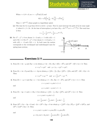


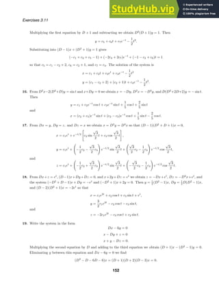

![-2 -1 1 2 x1
-2
-1
1
2
3
x2
Exercises 3.11
(c)
24. Write the system as
0.04i
2 + 30i2 + 10i3 = 50
0.02i
3 + 10i2 + 10i3 = 50
or
i
2 + 750i2 + 250i3 = 1250
i
3 + 500i2 + 500i3 = 2500.
In operator notation this becomes
(D + 750)i2 + 250i3 = 1250
500i2 + (D + 500)i3 = 2500.
Eliminating i3 we get
(D + 500)(D + 750) − 250(500)
i2 = (D + 250)(D + 1000)i2 = 0.
Thus
i2(t) = c1e−250t
+ c2e−1000t
.
Since i3 = 1
250 [1250 − (D + 750)i2], we have
i3(t) = −2c1e−250t
+ c2e−1000t
+ 5.
The initial conditions imply
i2(0) = c1 + c2 = 0
i3(0) = −2c1 + c2 + 5 = 0,
so c1 = 5
3 and c2 = −5
3 . Thus
i2(t) =
5
3
e−250t
−
5
3
e−1000t
i3(t) = −
10
3
e−250t
−
5
3
e−1000t
+ 5.
25. Equating Newton’s law with the net forces in the x- and y-directions gives m
d2
x
dt2
= 0 and m
d2
y
dt2
= −mg,
respectively. From mD2
x = 0 we obtain x(t) = c1t + c2, and from mD2
y = −mg or D2
y = −g we obtain
y(t) = −
1
2
gt2
+ c3t + c4.
26. From Newton’s second law in the x-direction we have
m
d2
x
dt2
= −k cos θ = −k
1
v
dx
dt
= −|c|
dx
dt
.
In the y-direction we have
m
d2
y
dt2
= −mg − k sin θ = −mg − k
1
v
dy
dt
= −mg − |c|
dy
dt
.
155](https://image.slidesharecdn.com/advancedengineeringmathematicssolutionsmanual-230807162553-1916df96/85/Advanced-Engineering-Mathematics-Solutions-Manual-pdf-155-320.jpg)
![Exercises 3.11
From mD2
x + |c|Dx = 0 we have D(mD + |c|)x = 0 so that (mD + |c|)x = c1. This is a first-order linear
equation. An integrating factor is e
|c|dt/m
e|c|t/m
so that
d
dt
[e|c|t/m
x] = c1e|c|t/m
and e|c|t
x = (c1m/|c|)e|c|t/m
+ c2. The general solution of this equation is x(t) = c3 + c2e|c|t/m
. From
(mD2
+ |c|D)y = −mg we have D(mD + |c|)y = −mg so that (mD + |c|)y = −mgt + c1. This is a first-order
linear equation with integrating factor e|c|t/m
. Thus
d
dt
[e|c|t/m
y] = (−mgt + c1)e|c|t/m
e|c|t/m
y = −
m2
g
|c|
te|c|t/m
+
m3
g
c2
e|c|t/m
+
c1m
|c|
e|c|t/m
+ c2
and
y(t) = −
m2
g
|c|
t +
m3
g
c2
+ c3 + c2e−|c|t/m
.
Chapter 3 Review Exercises
1. y = 0
2. Since yc = c1ex
+ c2e−x
, a particular solution for y
− y = 1 + ex
is yp = A + Bxex
.
3. True
4. True
5. 8 ft., since k = 4.
6. 2π/5, since 1
4 x
+ 6.25x = 0.
7. 5/4 m, since x = − cos 4t + 3
4 sin 4t.
8. From x(0) = (
√
2/2) sin φ = −1/2 we see that sin φ = −1/
√
2 , so φ is an angle in the third or fourth quadrant.
Since x
(t) =
√
2 cos(2t + φ), x
(0) =
√
2 cos φ = 1 and cos φ 0. Thus φ is in the fourth quadrant and
φ = −π/4.
9. They are linearly independent over (−∞, ∞) and linearly dependent over (0, ∞).
10. (a) Since f2(x) = 2 ln x = 2f1(x), the functions are linearly dependent.
(b) Since xn+1
is not a constant multiple of xn
, the functions are linearly independent.
(c) Since x + 1 is not a constant multiple of x, the functions are linearly independent.
(d) Since f1(x) = cos x cos(π/2) − sin x sin(π/2) = − sin x = −f2(x), the functions are linearly dependent.
(e) Since f1(x) = 0 · f2(x), the functions are linearly dependent.
(f) Since 2x is not a constant multiple of 2, the functions are linearly independent.
(g) Since 3(x2
) + 2(1 − x2
) − (2 + x2
) = 0, the functions are linearly dependent.
(h) since xex+1
+ 0(4x − 5)ex
− exex
= 0, the functions are linearly dependent.
11. (a) The auxiliary eqution is (m − 3)(m + 5)(m − 1) = m3
+ m2
− 17m + 15 = 0, so the differential equation is
y
+ y
− 17y
+ 15y = 0.
(b) The form of the auxiliary equation is
m(m − 1)(m − 2) + bm(m − 1) + cm + d = m3
+ (b − 3)m2
+ (c − b + 2)m + d = 0.
156](https://image.slidesharecdn.com/advancedengineeringmathematicssolutionsmanual-230807162553-1916df96/85/Advanced-Engineering-Mathematics-Solutions-Manual-pdf-156-320.jpg)
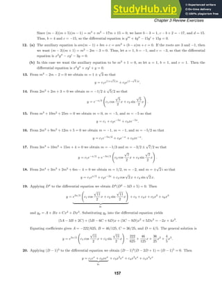
![Chapter 3 Review Exercises
and yp = Ax2
ex
+ Bx3
ex
+ Cx4
ex
. Substituting yp into the differential equation yields
12Cx2
ex
+ 6Bxex
+ 2Aex
= x2
ex
.
Equating coefficients gives A = 0, B = 0, and C = 1/12. The general solution is
y = c1ex
+ c2xex
+
1
12
x4
ex
.
21. Applying D(D2
+ 1) to the differential equation we obtain
D(D2
+ 1)(D3
− 5D2
+ 6D) = D2
(D2
+ 1)(D − 2)(D − 3) = 0.
Then
y = c1 + c2e2x
+ c3e3x
yc
+ c4x + c5 cos x + c6 sin x
and yp = Ax + B cos x + C sin x. Substituting yp into the differential equation yields
6A + (5B + 5C) cos x + (−5B + 5C) sin x = 8 + 2 sin x.
Equating coefficients gives A = 4/3, B = −1/5, and C = 1/5. The general solution is
y = c1 + c2e2x
+ c3e3x
+
4
3
x −
1
5
cos x +
1
5
sin x.
22. Applying D to the differential equation we obtain D(D3
− D2
) = D3
(D − 1) = 0. Then
y = c1 + c2x + c3ex
yc
+ c4x2
and yp = Ax2
. Substituting yp into the differential equation yields −2A = 6. Equating coefficients gives A = −3.
The general solution is
y = c1 + c2x + c3ex
− 3x2
.
23. The auxiliary equation is m2
− 2m + 2 = [m − (1 + i)][m − (1 − i)] = 0, so yc = c1ex
sin x + c2ex
cos x and
W =
ex
sin x ex
cos x
ex
cos x + ex
sin x −ex
sin x + ex
cos x
= −e2x
.
Identifying f(x) = ex
tan x we obtain
u
1 = −
(ex
cos x)(ex
tan x)
−e2x
= sin x
u
2 =
(ex
sin x)(ex
tan x)
−e2x
= −
sin2
x
cos x
= cos x − sec x.
Then u1 = − cos x, u2 = sin x − ln | sec x + tan x|, and
y = c1ex
sin x + c2ex
cos x − ex
sin x cos x + ex
sin x cos x − ex
cos x ln | sec x + tan x|
= c1ex
sin x + c2ex
cos x − ex
cos x ln | sec x + tan x|.
24. The auxiliary equation is m2
− 1 = 0, so yc = c1ex
+ c2e−x
and
W =
ex
e−x
ex
−e−x
= −2.
158](https://image.slidesharecdn.com/advancedengineeringmathematicssolutionsmanual-230807162553-1916df96/85/Advanced-Engineering-Mathematics-Solutions-Manual-pdf-158-320.jpg)
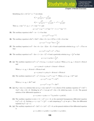
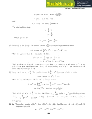

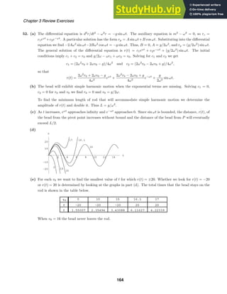
![Exercises 4.2
Solving for {y} we obtain
{y} =
2
(s − 1)(s2 + 25)
=
1
13
·
1
s − 1
−
1
13
s
s2 + 25
+
5
13
·
5
s2 + 25
.
Thus
y =
1
13
et
−
1
13
cos 5t +
5
13
sin 5t.
35. The Laplace transform of the differential equation is
s2
{y} − sy(0) − y
(0) + 5 [s {y} − y(0)] + 4 {y} = 0.
Solving for {y} we obtain
{y} =
s + 5
s2 + 5s + 4
=
4
3
1
s + 1
−
1
3
1
s + 4
.
Thus
y =
4
3
e−t
−
1
3
e−4t
.
36. The Laplace transform of the differential equation is
s2
{y} − sy(0) − y
(0) − 4 [s {y} − y(0)] =
6
s − 3
−
3
s + 1
.
Solving for {y} we obtain
{y} =
6
(s − 3)(s2 − 4s)
−
3
(s + 1)(s2 − 4s)
+
s − 5
s2 − 4s
=
5
2
·
1
s
−
2
s − 3
−
3
5
·
1
s + 1
+
11
10
·
1
s − 4
.
Thus
y =
5
2
− 2e3t
−
3
5
e−t
+
11
10
e4t
.
37. The Laplace transform of the differential equation is
s2
{y} − sy(0) + {y} =
2
s2 + 2
.
Solving for {y} we obtain
{y} =
2
(s2 + 1)(s2 + 2)
+
10s
s2 + 1
=
10s
s2 + 1
+
2
s2 + 1
−
2
s2 + 2
.
Thus
y = 10 cos t + 2 sin t −
√
2 sin
√
2 t.
38. The Laplace transform of the differential equation is
s2
{y} + 9 {y} =
1
s − 1
.
Solving for {y} we obtain
{y} =
1
(s − 1)(s2 + 9)
=
1
10
·
1
s − 1
−
1
10
·
1
s2 + 9
−
1
10
·
s
s2 + 9
.
Thus
y =
1
10
et
−
1
30
sin 3t −
1
10
cos 3t.
39. The Laplace transform of the differential equation is
2
s3
{y} − s2
(0) − sy
(0) − y
(0)
+ 3
s2
{y} − sy(0) − y
(0)
− 3[s {y} − y(0)] − 2 {y} =
1
s + 1
.
171](https://image.slidesharecdn.com/advancedengineeringmathematicssolutionsmanual-230807162553-1916df96/85/Advanced-Engineering-Mathematics-Solutions-Manual-pdf-171-320.jpg)
![Exercises 4.2
Solving for {y} we obtain
{y} =
2s + 3
(s + 1)(s − 1)(2s + 1)(s + 2)
=
1
2
1
s + 1
+
5
18
1
s − 1
−
8
9
1
s + 1/2
+
1
9
1
s + 2
.
Thus
y =
1
2
e−t
+
5
18
et
−
8
9
e−t/2
+
1
9
e−2t
.
40. The Laplace transform of the differential equation is
s3
{y} − s2
(0) − sy
(0) − y
(0) + 2
s2
{y} − sy(0) − y
(0)
− [s {y} − y(0)] − 2 {y} =
3
s2 + 9
.
Solving for {y} we obtain
{y} =
s2
+ 12
(s − 1)(s + 1)(s + 2)(s2 + 9)
=
13
60
1
s − 1
−
13
20
1
s + 1
+
16
39
1
s + 2
+
3
130
s
s2 + 9
−
1
65
3
s2 + 9
.
Thus
y =
13
60
et
−
13
20
e−t
+
16
39
e−2t
+
3
130
cos 3t −
1
65
sin 3t.
41. For y
+ 6y = e4t
the transfer function is W(s) = 1/(s + 6). The zero-input response is
y0(t) =
2
s + 6
= 2e−6t
,
and the zero-state response is
y1(t) =
1
(s − 4)(s + 6)
=
−
1
10
·
1
s + 6
+
1
10
·
1
s − 4
= −
1
10
e−6t
+
1
10
e4t
.
42. For y
− 4y
= 6e3t
− 3e−t
the transfer function is W(s) = 1/(s2
− 4s). The zero-input response is
y0(t) =
s − 5
s2 − 4s
=
5
4
·
1
s
−
1
4
·
1
s − 4
=
5
4
−
1
4
e4t
,
and the zero-state response is
y1(t) =
6
(s − 3)(s2 − 4s)
−
3
(s + 1)(s2 − 4s)
=
27
20
·
1
s − 4
−
2
s − 3
+
5
4
·
1
s
−
3
5
·
1
s + 1
=
27
20
e4t
− 2e3t
+
5
4
−
3
5
e−t
.
43. The Laplace transform of the differential equation is
s {y} + {y} =
s + 3
(s + 3)2 + 4
=
s + 3
s2 + 6s + 13
.
Solving for {y} we obtain
{y} =
s + 3
(s + 1)(s2 + 6s + 13)
=
1
4
·
1
s + 1
−
1
4
·
s + 1
s2 + 6s + 13
=
1
4
·
1
s + 1
−
1
4
s + 3
(s + 3)2 + 4
−
2
(s + 3)2 + 4
.
172](https://image.slidesharecdn.com/advancedengineeringmathematicssolutionsmanual-230807162553-1916df96/85/Advanced-Engineering-Mathematics-Solutions-Manual-pdf-172-320.jpg)
![Exercises 4.3
18.
5s
(s − 2)2
=
5(s − 2) + 10
(s − 2)2
=
5
s − 2
+
10
(s − 2)2
= 5e2t
+ 10te2t
19.
2s − 1
s2(s + 1)3
=
5
s
−
1
s2
−
5
s + 1
−
4
(s + 1)2
−
3
2
2
(s + 1)3
= 5 − t − 5e−t
− 4te−t
−
3
2
t2
e−t
20.
(s + 1)2
(s + 2)4
=
1
(s + 2)2
−
2
(s + 2)3
+
1
6
3!
(s + 2)4
= te−2t
− t2
e−2t
+
1
6
t3
e−2t
21. The Laplace transform of the differential equation is
s {y} − y(0) + 4 {y} =
1
s + 4
.
Solving for {y} we obtain {y} =
1
(s + 4)2
+
2
s + 4
. Thus
y = te−4t
+ 2e−4t
.
22. The Laplace transform of the differential equation is
s {y} − {y} =
1
s
+
1
(s − 1)2
.
Solving for {y} we obtain
{y} =
1
s(s − 1)
+
1
(s − 1)3
= −
1
s
+
1
s − 1
+
1
(s − 1)3
.
Thus
y = −1 + et
+
1
2
t2
et
.
23. The Laplace transform of the differential equation is
s2
{y} − sy(0) − y
(0) + 2
s {y} − y(0)
+ {y} = 0.
Solving for {y} we obtain
{y} =
s + 3
(s + 1)2
=
1
s + 1
+
2
(s + 1)2
.
Thus
y = e−t
+ 2te−t
.
24. The Laplace transform of the differential equation is
s2
{y} − sy(0) − y
(0) − 4 [s {y} − y(0)] + 4 {y} =
6
(s − 2)4
.
Solving for {y} we obtain {y} =
1
20
5!
(s − 2)6
. Thus, y =
1
20
t5
e2t
.
25. The Laplace transform of the differential equation is
s2
{y} − sy(0) − y
(0) − 6 [s {y} − y(0)] + 9 {y} =
1
s2
.
Solving for {y} we obtain
{y} =
1 + s2
s2(s − 3)2
=
2
27
1
s
+
1
9
1
s2
−
2
27
1
s − 3
+
10
9
1
(s − 3)2
.
Thus
y =
2
27
+
1
9
t −
2
27
e3t
+
10
9
te3t
.
174](https://image.slidesharecdn.com/advancedengineeringmathematicssolutionsmanual-230807162553-1916df96/85/Advanced-Engineering-Mathematics-Solutions-Manual-pdf-174-320.jpg)
![Exercises 4.3
26. The Laplace transform of the differential equation is
s2
{y} − sy(0) − y
(0) − 4 [s {y} − y(0)] + 4 {y} =
6
s4
.
Solving for {y} we obtain
{y} =
s5
− 4s4
+ 6
s4(s − 2)2
=
3
4
1
s
+
9
8
1
s2
+
3
4
2
s3
+
1
4
3!
s4
+
1
4
1
s − 2
−
13
8
1
(s − 2)2
.
Thus
y =
3
4
+
9
8
t +
3
4
t2
+
1
4
t3
+
1
4
e2t
−
13
8
te2t
.
27. The Laplace transform of the differential equation is
s2
{y} − sy(0) − y
(0) − 6 [s {y} − y(0)] + 13 {y} = 0.
Solving for {y} we obtain
{y} = −
3
s2 − 6s + 13
= −
3
2
2
(s − 3)2 + 22
.
Thus
y = −
3
2
e3t
sin 2t.
28. The Laplace transform of the differential equation is
2
s2
{y} − sy(0)
+ 20
s {y} − y(0)
+ 51 {y} = 0.
Solving for {y} we obtain
{y} =
4s + 40
2s2 + 20s + 51
=
2s + 20
(s + 5)2 + 1/2
=
2(s + 5)
(s + 5)2 + 1/2
+
10
(s + 5)2 + 1/2
.
Thus
y = 2e−5t
cos(t/
√
2 ) + 10
√
2 e−5t
sin(t/
√
2 ).
29. The Laplace transform of the differential equation is
s2
{y} − sy(0) − y
(0) − [s {y} − y(0)] =
s − 1
(s − 1)2 + 1
.
Solving for {y} we obtain
{y} =
1
s(s2 − 2s + 2)
=
1
2
1
s
−
1
2
s − 1
(s − 1)2 + 1
+
1
2
1
(s − 1)2 + 1
.
Thus
y =
1
2
−
1
2
et
cos t +
1
2
et
sin t.
30. The Laplace transform of the differential equation is
s2
{y} − sy(0) − y
(0) − 2 [s {y} − y(0)] + 5 {y} =
1
s
+
1
s2
.
Solving for {y} we obtain
{y} =
4s2
+ s + 1
s2(s2 − 2s + 5)
=
7
25
1
s
+
1
5
1
s2
+
−7s/25 + 109/25
s2 − 2s + 5
=
7
25
1
s
+
1
5
1
s2
−
7
25
s − 1
(s − 1)2 + 22
+
51
25
2
(s − 1)2 + 22
.
175](https://image.slidesharecdn.com/advancedengineeringmathematicssolutionsmanual-230807162553-1916df96/85/Advanced-Engineering-Mathematics-Solutions-Manual-pdf-175-320.jpg)
![Exercises 4.3
Solving for {y} we obtain
{y} =
1
s2(s + 2)
− e−s s + 1
s2(s + 1)
= −
1
4
1
s
+
1
2
1
s2
+
1
4
1
s + 2
− e−s
1
4
1
s
+
1
2
1
s2
−
1
4
1
s + 2
.
Thus
y = −
1
4
+
1
2
t +
1
4
e−2t
−
1
4
+
1
2
(t − 1) −
1
4
e−2(t−1)
(t − 1).
66. The Laplace transform of the differential equation is
s2
{y} − sy(0) − y
(0) + 4 {y} =
1
s
−
e−s
s
.
Solving for {y} we obtain
{y} =
1 − s
s(s2 + 4)
− e−s 1
s(s2 + 4)
=
1
4
1
s
−
1
4
s
s2 + 4
−
1
2
2
s2 + 4
− e−s
1
4
1
s
−
1
4
s
s2 + 4
.
Thus
y =
1
4
−
1
4
cos 2t −
1
2
sin 2t −
1
4
−
1
4
cos 2(t − 1)
(t − 1).
67. The Laplace transform of the differential equation is
s2
{y} − sy(0) − y
(0) + 4 {y} = e−2πs 1
s2 + 1
.
Solving for {y} we obtain
{y} =
s
s2 + 4
+ e−2πs
1
3
1
s2 + 1
−
1
6
2
s2 + 4
.
Thus
y = cos 2t +
1
3
sin(t − 2π) −
1
6
sin 2(t − 2π)
(t − 2π).
68. The Laplace transform of the differential equation is
s2
{y} − sy(0) − y
(0) − 5 [s {y} − y(0)] + 6 {y} =
e−s
s
.
Solving for {y} we obtain
{y} = e−s 1
s(s − 2)(s − 3)
+
1
(s − 2)(s − 3)
= e−s
1
6
1
s
−
1
2
1
s − 2
+
1
3
1
s − 3
−
1
s − 2
+
1
s − 3
.
Thus
y =
1
6
−
1
2
e2(t−1)
+
1
3
e3(t−1)
(t − 1) + e3t
− e2t
.
69. The Laplace transform of the differential equation is
s2
{y} − sy(0) − y
(0) + {y} =
e−πs
s
−
e−2πs
s
.
Solving for {y} we obtain
{y} = e−πs
1
s
−
s
s2 + 1
− e−2πs
1
s
−
s
s2 + 1
+
1
s2 + 1
.
Thus
y = [1 − cos(t − π)] (t − π) − [1 − cos(t − 2π)] (t − 2π) + sin t.
180](https://image.slidesharecdn.com/advancedengineeringmathematicssolutionsmanual-230807162553-1916df96/85/Advanced-Engineering-Mathematics-Solutions-Manual-pdf-180-320.jpg)

![1 2 3 4 5 6
t
-0.2
0.2
i
1 2 3 4 5 6
t
1
q
Exercises 4.3
Solving for {i} we obtain
{i} =
1
(s2 + 1)(s + 10)
+
s
(s2 + 1)(s + 10)
e−3πs/2
=
1
101
1
s + 10
−
s
s2 + 1
+
10
s2 + 1
+
1
101
−10
s + 10
+
10s
s2 + 1
+
1
s2 + 1
e−3πs/2
.
Thus
i(t) =
1
101
e−10t
− cos t + 10 sin t
+
1
101
−10e−10(t−3π/2)
+ 10 cos
t −
3π
2
+ sin
t −
3π
2
t −
3π
2
.
(b)
The maximum value of i(t) is approximately 0.1 at t = 1.7, the minimum is approximately −0.1 at 4.7.
76. (a) The differential equation is
50
dq
dt
+
1
0.01
q = E0[ (t − 1) − (t − 3)], q(0) = 0
or
50
dq
dt
+ 100q = E0[ (t − 1) − (t − 3)], q(0) = 0.
The Laplace transform of this equation is
50s {q} + 100 {q} = E0
1
s
e−s
−
1
s
e−3s
.
Solving for {q} we obtain
{q} =
E0
50
e−s
s(s + 2)
−
e−3s
s(s + 2)
=
E0
50
1
2
1
s
−
1
s + 2
e−s
−
1
2
1
s
−
1
s + 2
e−3s
.
Thus
q(t) =
E0
100
1 − e−2(t−1)
(t − 1) −
1 − e−2(t−3)
(t − 3) .
(b)
The maximum value of q(t) is approximately 1 at t = 3.
77. The differential equation is
EI
d4
y
dx4
= w0[1 − (x − L/2)].
Taking the Laplace transform of both sides and using y(0) = y
(0) = 0 we obtain
s4
{y} − sy
(0) − y
(0) =
w0
EI
1
s
1 − e−Ls/2
.
183](https://image.slidesharecdn.com/advancedengineeringmathematicssolutionsmanual-230807162553-1916df96/85/Advanced-Engineering-Mathematics-Solutions-Manual-pdf-183-320.jpg)
![Exercises 4.3
Letting y
(0) = c1 and y
(0) = c2 we have
{y} =
c1
s3
+
c2
s4
+
w0
EI
1
s5
1 − e−Ls/2
so that
y(x) =
1
2
c1x2
+
1
6
c2x3
+
1
24
w0
EI
x4
−
x −
L
2
4
x −
L
2
.
To find c1 and c2 we compute
y
(x) = c1 + c2x +
1
2
w0
EI
x2
−
x −
L
2
2
x −
L
2
and
y
(x) = c2 +
w0
EI
x −
x −
L
2
x −
L
2
.
Then y
(L) = y
(L) = 0 yields the system
c1 + c2L +
1
2
w0
EI
L2
−
L
2
2
= c1 + c2L +
3
8
w0L2
EI
= 0
c2 +
w0
EI
L
2
= c2 +
1
2
w0L
EI
= 0.
Solving for c1 and c2 we obtain c1 = 1
8 w0L2
/EI and c2 = −1
2 w0L/EI. Thus
y(x) =
w0
EI
1
16
L2
x2
−
1
12
Lx3
+
1
24
x4
−
1
24
x −
L
2
4
x −
L
2
.
78. The differential equation is
EI
d4
y
dx4
= w0[ (x − L/3) − (x − 2L/3)].
Taking the Laplace transform of both sides and using y(0) = y
(0) = 0 we obtain
s4
{y} − sy
(0) − y
(0) =
w0
EI
1
s
e−Ls/3
− e−2Ls/3
.
Letting y
(0) = c1 and y
(0) = c2 we have
{y} =
c1
s3
+
c2
s4
+
w0
EI
1
s5
e−Ls/3
− e−2Ls/3
so that
y(x) =
1
2
c1x2
+
1
6
c2x3
+
1
24
w0
EI
x −
L
3
4
x −
L
3
−
x −
2L
3
4
x −
2L
3
.
To find c1 and c2 we compute
y
(x) = c1 + c2x +
1
2
w0
EI
x −
L
3
2
x −
L
3
−
x −
2L
3
2
x −
2L
3
and
y
(x) = c2 +
w0
EI
x −
L
3
x −
L
3
−
x −
2L
3
x −
2L
3
.
Then y
(L) = y
(L) = 0 yields the system
c1 + c2L +
1
2
w0
EI
2L
3
2
−
L
3
2
= c1 + c2L +
1
6
w0L2
EI
= 0
c2 +
w0
EI
2L
3
−
L
3
= c2 +
1
3
w0L
EI
= 0.
184](https://image.slidesharecdn.com/advancedengineeringmathematicssolutionsmanual-230807162553-1916df96/85/Advanced-Engineering-Mathematics-Solutions-Manual-pdf-184-320.jpg)
![Exercises 4.3
Solving for c1 and c2 we obtain c1 = 1
6 w0L2
/EI and c2 = −1
3 w0L/EI. Thus
y(x) =
w0
EI
1
12
L2
x2
−
1
18
Lx3
+
1
24
x −
L
3
4
x −
L
3
−
x −
2L
3
4
x −
2L
3
.
79. The differential equation is
EI
d4
y
dx4
=
2w0
L
L
2
− x +
x −
L
2
x −
L
2
.
Taking the Laplace transform of both sides and using y(0) = y
(0) = 0 we obtain
s4
{y} − sy
(0) − y
(0) =
2w0
EIL
L
2s
−
1
s2
+
1
s2
e−Ls/2
.
Letting y
(0) = c1 and y
(0) = c2 we have
{y} =
c1
s3
+
c2
s4
+
2w0
EIL
L
2s5
−
1
s6
+
1
s6
e−Ls/2
so that
y(x) =
1
2
c1x2
+
1
6
c2x3
+
2w0
EIL
L
48
x4
−
1
120
x5
+
1
120
x −
L
2
x −
L
2
=
1
2
c1x2
+
1
6
c2x3
+
w0
60EIL
5L
2
x4
− x5
+
x −
L
2
5
x −
L
2
.
To find c1 and c2 we compute
y
(x) = c1 + c2x +
w0
60EIL
30Lx2
− 20x3
+ 20
x −
L
2
3
x −
L
2
and
y
(x) = c2 +
w0
60EIL
60Lx − 60x2
+ 60
x −
L
2
2
x −
L
2
.
Then y
(L) = y
(L) = 0 yields the system
c1 + c2L +
w0
60EIL
30L3
− 20L3
+
5
2
L3
= c1 + c2L +
5w0L2
24EI
= 0
c2 +
w0
60EIL
[60L2
− 60L2
+ 15L2
] = c2 +
w0L
4EI
= 0.
Solving for c1 and c2 we obtain c1 = w0L2
/24EI and c2 = −w0L/4EI. Thus
y(x) =
w0L2
48EI
x2
−
w0L
24EI
+
w0
60EIL
5L
2
x4
− x5
+
x −
L
2
5
x −
L
2
.
80. The differential equation is
EI
d4
y
dx4
= w0[1 − (x − L/2)].
Taking the Laplace transform of both sides and using y(0) = y
(0) = 0 we obtain
s4
{y} − sy
(0) − y
(0) =
w0
EI
1
s
1 − e−Ls/2
.
Letting y
(0) = c1 and y
(0) = c2 we have
{y} =
c1
s3
+
c2
s4
+
w0
EI
1
s5
1 − e−Ls/2
185](https://image.slidesharecdn.com/advancedengineeringmathematicssolutionsmanual-230807162553-1916df96/85/Advanced-Engineering-Mathematics-Solutions-Manual-pdf-185-320.jpg)
![Exercises 4.3
so that
y(x) =
1
2
c1x2
+
1
6
c2x3
+
1
24
w0
EI
x4
−
x −
L
2
4
x −
L
2
.
To find c1 and c2 we compute
y
(x) = c1 + c2x +
1
2
w0
EI
x2
−
x −
L
2
2
x −
L
2
.
Then y(L) = y
(L) = 0 yields the system
1
2
c1L2
+
1
6
c2L3
+
1
24
w0
EI
L4
−
L
2
4
=
1
2
c1L2
+
1
6
c2L3
+
5w0
128EI
L4
= 0
c1 + c2L +
1
2
w0
EI
L2
−
L
2
2
= c1 + c2L +
3w0
8EI
L2
= 0.
Solving for c1 and c2 we obtain c1 = 9
128 w0L2
/EI and c2 = − 57
128 w0L/EI. Thus
y(x) =
w0
EI
9
256
L2
x2
−
19
256
Lx3
+
1
24
x4
−
1
24
x −
L
2
4
x −
L
2
.
81. From Theorem 4.6 we have {tekti
} = 1/(s − ki)2
. Then, using Euler’s formula,
{tekti
} = {t cos kt + it sin kt} = {t cos kt} + i {t sin kt}
=
1
(s − ki)2
=
(s + ki)2
(s2 + k2)2
=
s2
− k2
(s2 + k2)2
+ i
2ks
(s2 + k2)2
.
Equating real and imaginary parts we have
{t cos kt} =
s2
− k2
(s2 + k2)2
and {t sin kt} =
2ks
(s2 + k2)2
.
82. The Laplace transform of the differential equation is
s2
{x} + ω2
{x} =
s
s2 + ω2
.
Solving for {x} we obtain {x} = s/(s2
+ ω2
)2
. Thus x = (1/2ω)t sin ωt.
Exercises 4.4
1. {t cos 2t} = −
d
ds
s
s2 + 4
=
s2
− 4
(s2 + 4)
2
2. {t sinh 3t} = −
d
ds
3
s2 − 9
=
6s
(s2 − 9)
2
3. {t2
sinh t} =
d2
ds2
1
s2 − 1
=
6s2
+ 2
(s2 − 1)
3
4. {t2
cos t} =
d2
ds2
s
s2 + 1
=
d
ds
1 − s2
(s2 + 1)2
=
2s
s2
− 3
(s2 + 1)
3
5.
te2t
sin 6t
= −
d
ds
6
(s − 2)2 + 36
=
12(s − 2)
[(s − 2)2 + 36]
2
186](https://image.slidesharecdn.com/advancedengineeringmathematicssolutionsmanual-230807162553-1916df96/85/Advanced-Engineering-Mathematics-Solutions-Manual-pdf-186-320.jpg)
![Exercises 4.4
6.
te−3t
cos 3t
= −
d
ds
s + 3
(s + 3)2 + 9
=
(s + 3)2
− 9
[(s + 3)2 + 9]
2
7.
1 ∗ t3
=
1
s
3!
s4
=
6
s5
8.
t2
∗ tet
=
2
s3(s − 1)2
9.
e−t
∗ et
cos t
=
s − 1
(s + 1) [(s − 1)2 + 1]
10.
e2t
∗ sin t
=
1
(s − 2)(s2 + 1)
11.
t
0
eτ
dτ
=
1
s
{et
} =
1
s(s − 1)
12.
t
0
cos τ dτ
=
1
s
{cos t} =
s
s(s2 + 1)
=
1
s2 + 1
13.
t
0
e−τ
cos τ dτ
=
1
s
e−t
cos t
=
1
s
s + 1
(s + 1)2 + 1
=
s + 1
s (s2 + 2s + 2)
14.
t
0
τ sin τ dτ
=
1
s
{t sin t} =
1
s
−
d
ds
1
s2 + 1
= −
1
s
−2s
(s2 + 1)
2 =
2
(s2 + 1)
2
15.
t
0
τet−τ
dτ
= {t} {et
} =
1
s2(s − 1)
16.
t
0
sin τ cos(t − τ) dτ
= {sin t} {cos t} =
s
(s2 + 1)
2
17.
t
t
0
sin τ dτ
= −
d
ds
t
0
sin τ dτ
= −
d
ds
1
s
1
s2 + 1
=
3s2
+ 1
s2 (s2 + 1)
2
18.
t
t
0
τe−τ
dτ
= −
d
ds
t
t
0
τe−τ
dτ
= −
d
ds
1
s
1
(s + 1)2
=
3s + 1
s2(s + 1)3
19. (a)
1
s(s − 1)
=
1/(s − 1)
s
=
t
0
eτ
dτ = et
− 1
(b)
1
s2(s − 1)
=
1/s(s − 1)
s
=
t
0
(eτ
− 1)dτ = et
− t − 1
(c)
1
s3(s − 1)
=
1/s2
(s − 1)
s
=
t
0
(eτ
− τ − 1)dτ = et
−
1
2
t2
− t − 1
20. (a) The result in (4) is {F(s)G(s)} = f ∗ g, so identify
F(s) =
2k3
(s2 + k2)2
and G(s) =
4s
s2 + k2
.
Then
f(t) = sin kt − kt cos kt and g(t) = 4 cos kt
so
8k3
s
(s2 + k2)2
= {F(s)G(s)} = f ∗ g = 4
t
0
f(τ)g(t − τ)dt
= 4
t
0
(sin kτ − kτ cos kτ) cos k(t − τ)dτ.
187](https://image.slidesharecdn.com/advancedengineeringmathematicssolutionsmanual-230807162553-1916df96/85/Advanced-Engineering-Mathematics-Solutions-Manual-pdf-187-320.jpg)
![Exercises 4.4
Using a CAS to evaluate the integral we get
8k3
s
(s2 + k2)3
= t sin kt − kt2
cos kt.
(b) Observe from part (a) that
t(sin kt − kt cos kt)
=
8k3
s
(s2 + k2)3
,
and from Theorem 4.8 that
tf(t)
= −F
(s). We saw in (5) that {sin kt−kt cos kt} = 2k3
/(s2
+k2
)2
,
so
t(sin kt − kt cos kt)
= −
d
ds
2k3
(s2 + k2)2
=
8k3
s
(s2 + k2)3
.
21. f(t) = −
1
t
d
ds
[ln(s − 3) − ln(s + 1)]
= −
1
t
1
s − 3
−
1
s + 1
= −
1
t
e3t
− e−t
22. f(t) = −
1
t
d
ds
ln
s2
+ 1
− ln
s2
+ 4
= −
1
t
2s
s2 + 1
−
2s
s2 + 22
= −
1
t
(2 cos t − 2 cos 2t)
23. {f(t)} =
1
1 − e−2as
a
0
e−st
dt −
2a
a
e−st
dt
=
(1 − e−as
)2
s(1 − e−2as)
=
1 − e−as
s(1 + e−as)
24. {f(t)} =
1
1 − e−2as
a
0
e−st
dt =
1
s(1 + e−as)
25. {f(t)} =
1
1 − e−bs
b
0
a
b
te−st
dt =
a
s
1
bs
−
1
ebs − 1
26. {f(t)} =
1
1 − e−2s
1
0
te−st
dt +
2
1
(2 − t)e−st
dt
=
1 − e−s
s2(1 − e−2s)
27. {f(t)} =
1
1 − e−πs
π
0
e−st
sin t dt =
1
s2 + 1
·
eπs/2
+ e−πs/2
eπs/2 − e−πs/2
=
1
s2 + 1
coth
πs
2
28. {f(t)} =
1
1 − e−2πs
π
0
e−st
sin t dt =
1
s2 + 1
·
1
1 − e−πs
29. The Laplace transform of the differential equation is
s {y} + {y} =
2s
(s2 + 1)2
.
Solving for {y} we obtain
{y} =
2s
(s + 1)(s2 + 1)2
= −
1
2
1
s + 1
−
1
2
1
s2 + 1
+
1
2
s
s2 + 1
+
1
(s2 + 1)2
+
s
(s2 + 1)2
.
Thus
y(t) = −
1
2
e−t
−
1
2
sin t +
1
2
cos t +
1
2
(sin t − t cos t) +
1
2
t sin t
= −
1
2
e−t
+
1
2
cos t −
1
2
t cos t +
1
2
t sin t.
30. The Laplace transform of the differential equation is
s {y} − {y} =
2(s − 1)
((s2 − 1)2 + 1)2
.
188](https://image.slidesharecdn.com/advancedengineeringmathematicssolutionsmanual-230807162553-1916df96/85/Advanced-Engineering-Mathematics-Solutions-Manual-pdf-188-320.jpg)


![π 2π t
x
−3
3
4π
2π
t
x
−5
5
Exercises 4.4
and
x(t) = 2
1 − e−t
cos 3t −
1
3
e−t
sin 3t
+ 4
∞
!
n=1
(−1)n
1 − e−(t−nπ)
cos 3(t − nπ)
−
1
3
e−(t−nπ)
sin 3(t − nπ)
(t − nπ).
The graph of x(t) on the interval [0, 2π) is shown below.
52. The differential equation is x
+ 2x
+ x = 5f(t), where f(t) is the square wave function with a = π. Using the
initial conditions x(0) = x
(0) = 0 and taking the Laplace transform, we obtain
(s2
+ 2s + 1) {x(t)} =
5
s
1
1 + e−πs
=
5
s
(1 − e−πs
+ e−2πs
− e−3πs
+ e−4πs
− · · ·)
=
5
s
∞
!
n=0
(−1)n
e−nπs
.
Then
{x(t)} =
5
s(s + 1)2
∞
!
n=0
(−1)n
e−nπs
= 5
∞
!
n=0
(−1)n
1
s
−
1
s + 1
−
1
(s + 1)2
e−nπs
and
x(t) = 5
∞
!
n=0
(−1)n
(1 − e−(t−nπ)
− (t − nπ)e−(t−nπ)
) (t − nπ).
The graph of x(t) on the interval [0, 4π) is shown below.
53. Let u = t − τ so that du = dτ and
f ∗ g =
t
0
f(τ)g(t − τ) dτ = −
0
t
f(t − u)g(u)du = g ∗ f.
54. f ∗ (g + h) =
t
0
f(τ)[g(t − τ) + h(t − τ)] dτ =
t
0
f(τ)g(t − τ) dτ +
t
0
f(τ)h(t − τ) dτ
=
t
0
f(τ)[g(t − τ) + h(t − τ)] dτ = f ∗ g + f ∗ h
195](https://image.slidesharecdn.com/advancedengineeringmathematicssolutionsmanual-230807162553-1916df96/85/Advanced-Engineering-Mathematics-Solutions-Manual-pdf-195-320.jpg)
![t
q
−5
5
π 3π
Exercises 4.4
55. (a) The output for the first three lines of the program are
9y[t] + 6y
[t] + y
[t] == t sin[t]
1 − 2s + 9Y + s2
Y + 6(−2 + sY ) ==
2s
(1 + s2)2
Y → −
−11 − 4s − 22s2
− 4s3
− 11s4
− 2s5
(1 + s2)2(9 + 6s + s2)
The fourth line is the same as the third line with Y → removed. The final line of output shows a solution
involving complex coefficients of eit
and e−it
. To get the solution in more standard form write the last line
as two lines:
euler = {Eˆ(I t) - Cos[t] + I Sin[t], Eˆ(-I t) - Cos[t] - I Sin[t]}
InverseLaplaceTransform[Y,s,t]/.euler//Expand
We see that the solution is
y(t) =
487
250
+
247
50
t
e−3t
+
1
250
(13 cos t − 15t cos t − 9 sin t + 20t sin t) .
(b) The solution is
y(t) =
1
6
et
−
1
6
e−t/2
cos
√
15 t −
3/5
6
e−t/2
sin
√
15 t.
(c) The solution is
q(t) = 1 − cos t + (6 − 6 cos t) (t − 3π) − (4 + 4 cos t) (t − π).
Exercises 4.5
1. The Laplace transform of the differential equation yields
{y} =
1
s − 3
e−2s
so that
y = e3(t−2)
(t − 2).
2. The Laplace transform of the differential equation yields
{y} =
2
s + 1
+
e−s
s + 1
so that
y = 2e−t
+ e−(t−1)
(t − 1).
3. The Laplace transform of the differential equation yields
{y} =
1
s2 + 1
1 + e−2πs
196](https://image.slidesharecdn.com/advancedengineeringmathematicssolutionsmanual-230807162553-1916df96/85/Advanced-Engineering-Mathematics-Solutions-Manual-pdf-196-320.jpg)
![Exercises 4.5
so that
y = sin t + sin t (t − 2π).
4. The Laplace transform of the differential equation yields
{y} =
1
4
4
s2 + 16
e−2πs
so that
y =
1
4
sin 4(t − 2π) (t − 2π).
5. The Laplace transform of the differential equation yields
{y} =
1
s2 + 1
e−πs/2
+ e−3πs/2
so that
y = sin
t −
π
2
t −
π
2
+ sin
t −
3π
2
t −
3π
2
= − cos t
t −
π
2
+ cos t
t −
π
2
.
6. The Laplace transform of the differential equation yields
{y} =
s
s2 + 1
+
1
s2 + 1
(e−2πs
+ e−4πs
)
so that
y = cos t + sin t[ (t − 2π) + (t − 4π)].
7. The Laplace transform of the differential equation yields
{y} =
1
s2 + 2s
(1 + e−s
) =
1
2
1
s
−
1
2
1
s + 2
(1 + e−s
)
so that
y =
1
2
−
1
2
e−2t
+
1
2
−
1
2
e−2(t−1)
(t − 1).
8. The Laplace transform of the differential equation yields
{y} =
s + 1
s2(s − 2)
+
1
s(s − 2)
e−2s
=
3
4
1
s − 2
−
3
4
1
s
−
1
2
1
s2
+
1
2
1
s − 2
−
1
2
1
s
e−2s
so that
y =
3
4
e2t
−
3
4
−
1
2
t +
1
2
e2(t−2)
−
1
2
(t − 2).
9. The Laplace transform of the differential equation yields
{y} =
1
(s + 2)2 + 1
e−2πs
so that
y = e−2(t−2π)
sin t (t − 2π).
10. The Laplace transform of the differential equation yields
{y} =
1
(s + 1)2
e−s
so that
y = (t − 1)e−(t−1)
(t − 1).
197](https://image.slidesharecdn.com/advancedengineeringmathematicssolutionsmanual-230807162553-1916df96/85/Advanced-Engineering-Mathematics-Solutions-Manual-pdf-197-320.jpg)


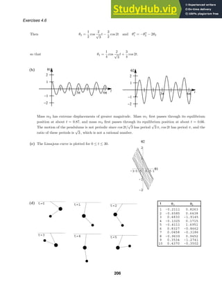

![Chapter 4 Review Exercises
12. {sin 2t (t − π)} = {sin 2(t − π) (t − π)} =
2
s2 + 4
e−πs
13.
20
s6
=
1
6
5!
s6
=
1
6
t5
14.
1
3s − 1
=
1
3
1
s − 1/3
=
1
3
et/3
15.
1
(s − 5)3
=
1
2
2
(s − 5)3
=
1
2
t2
e5t
16.
1
s2 − 5
=
−
1
√
5
1
s +
√
5
+
1
√
5
1
s −
√
5
= −
1
√
5
e−
√
5 t
+
1
√
5
e
√
5 t
17.
s
s2 − 10s + 29
=
s − 5
(s − 5)2 + 22
+
5
2
2
(s − 5)2 + 22
= e5t
cos 2t +
5
2
e5t
sin 2t
18.
1
s2
e−5s
= (t − 5) (t − 5)
19.
s + π
s2 + π2
e−s
=
s
s2 + π2
e−s
+
π
s2 + π2
e−s
= cos π(t − 1) (t − 1) + sin π(t − 1) (t − 1)
20.
1
L2s2 + n2π2
=
1
L2
L
nπ
nπ/L
s2 + (n2π2)/L2
=
1
Lnπ
sin
nπ
L
t
21.
e−5t
exists for s −5.
22.
te8t
f(t)
= −
d
ds
F(s − 8).
23. {eat
f(t − k) (t − k)} = e−ks
{ea(t+k)
f(t)} = e−ks
eak
{eat
f(t)} = e−k(s−a)
F(s − a)
24.
t
0
eaτ
f(τ) dτ
=
1
s
{eat
f(t)} =
F(s − a)
s
, whereas
eat
t
0
f(τ) dτ
=
t
0
f(τ) dτ
s→s−a
=
F(s)
s
s→s−a
=
F(s − a)
s − a
.
25. f(t) (t − t0)
26. f(t) − f(t) (t − t0)
27. f(t − t0) (t − t0)
28. f(t) − f(t) (t − t0) + f(t) (t − t1)
29. f(t) = t − [(t − 1) + 1] (t − 1) + (t − 1) − (t − 4) = t − (t − 1) (t − 1) − (t − 4)
{f(t)} =
1
s2
−
1
s2
e−s
−
1
s
e−4s
et
f(t)
=
1
(s − 1)2
−
1
(s − 1)2
e−(s−1)
−
1
s − 1
e−4(s−1)
30. f(t) = sin t (t − π) − sin t (t − 3π) = − sin(t − π) (t − π) + sin(t − 3π) (t − 3π)
{f(t)} = −
1
s2 + 1
e−πs
+
1
s2 + 1
e−3πs
et
f(t)
= −
1
(s − 1)2 + 1
e−π(s−1)
+
1
(s − 1)2 + 1
e−3π(s−1)
208](https://image.slidesharecdn.com/advancedengineeringmathematicssolutionsmanual-230807162553-1916df96/85/Advanced-Engineering-Mathematics-Solutions-Manual-pdf-208-320.jpg)
![Chapter 4 Review Exercises
31. f(t) = 2 − 2 (t − 2) + [(t − 2) + 2] (t − 2) = 2 + (t − 2) (t − 2)
{f(t)} =
2
s
+
1
s2
e−2s
et
f(t)
=
2
s − 1
+
1
(s − 1)2
e−2(s−1)
32. f(t) = t − t (t − 1) + (2 − t) (t − 1) − (2 − t) (t − 2) = t − 2(t − 1) (t − 1) + (t − 2) (t − 2)
{f(t)} =
1
s2
−
2
s2
e−s
+
1
s2
e−2s
et
f(t)
=
1
(s − 1)2
−
2
(s − 1)2
e−(s−1)
+
1
(s − 1)2
e−2(s−1)
33. Taking the Laplace transform of the differential equation we obtain
{y} =
5
(s − 1)2
+
1
2
2
(s − 1)3
so that
y = 5tet
+
1
2
t2
et
.
34. Taking the Laplace transform of the differential equation we obtain
{y} =
1
(s − 1)2(s2 − 8s + 20)
=
6
169
1
s − 1
+
1
13
1
(s − 1)2
−
6
169
s − 4
(s − 4)2 + 22
+
5
338
2
(s − 4)2 + 22
so that
y =
6
169
et
+
1
13
tet
−
6
169
e4t
cos 2t +
5
338
e4t
sin 2t.
35. Taking the Laplace transform of the given differential equation we obtain
{y} =
s3
+ 6s2
+ 1
s2(s + 1)(s + 5)
−
1
s2(s + 1)(s + 5)
e−2s
−
2
s(s + 1)(s + 5)
e−2s
= −
6
25
·
1
s
+
1
5
·
1
s2
+
3
2
·
1
s + 1
−
13
50
·
1
s + 5
−
−
6
25
·
1
s
+
1
5
·
1
s2
+
1
4
·
1
s + 1
−
1
100
·
1
s + 5
e−2s
−
2
5
·
1
5
−
1
2
·
1
s + 1
+
1
10
·
1
s + 5
e−2s
so that
y = −
6
25
+
1
5
t2
+
3
2
e−t
−
13
50
e−5t
−
4
25
(t − 2) −
1
5
(t − 2)2
(t − 2)
+
1
4
e−(t−2)
(t − 2) −
9
100
e−5(t−2)
(t − 2).
36. Taking the Laplace transform of the differential equation we obtain
{y} =
s3
+ 2
s3(s − 5)
−
2 + 2s + s2
s3(s − 5)
e−s
= −
2
125
1
s
−
2
25
1
s2
−
1
5
2
s3
+
127
125
1
s − 5
−
−
37
125
1
s
−
12
25
1
s2
−
1
5
2
s3
+
37
125
1
s − 5
e−s
so that
y = −
2
125
−
2
25
t −
1
5
t2
+
127
125
e5t
−
−
37
125
−
12
25
(t − 1) −
1
5
(t − 1)2
+
37
125
e5(t−1)
(t − 1).
209](https://image.slidesharecdn.com/advancedengineeringmathematicssolutionsmanual-230807162553-1916df96/85/Advanced-Engineering-Mathematics-Solutions-Manual-pdf-209-320.jpg)

![Exercises 5.1
9.
∞
n=1
2ncnxn−1
+
∞
n=0
6cnxn+1
= 2 · 1 · c1x0
+
∞
n=2
2ncnxn−1
k=n−1
+
∞
n=0
6cnxn+1
k=n+1
= 2c1 +
∞
k=1
2(k + 1)ck+1xk
+
∞
k=1
6ck−1xk
= 2c1 +
∞
k=1
[2(k + 1)ck+1 + 6ck−1]xk
10.
∞
n=2
n(n − 1)cnxn
+ 2
∞
n=2
n(n − 1)cnxn−2
+ 3
∞
n=1
ncnxn
= 2 · 2 · 1c2x0
+ 2 · 3 · 2c3x
+ 3 · 1 · c1x
+
∞
n=2
n(n − 1)cnxn
k=n
+2
∞
n=4
n(n − 1)cnxn−2
k=n−2
+3
∞
n=2
ncnxn
k=n
= 4c2 + (12c3 + (12c3 + 3c1)x +
∞
n=2
k(k − 1)ckxk
+ 2
∞
n=2
(k + 2)(k + 1)ck+2xk
+ 3
∞
n=2
kckxk
= 4c2 + (3c1 + 12c3)x +
∞
n=2
[k(k − 1) + 3k]ck + 2(k + 2)(k + 1)ck+2 xk
= 4c2 + (3c1 + 12c3)x +
∞
n=2
k(k + 2)ck + 2(k + 1)(k + 2)ck+2 xk
11. y
=
∞
n=1
(−1)n+1
xn−1
, y
=
∞
n=2
(−1)n+1
(n − 1)xn−2
(x + 1)y
+ y
= (x + 1)
∞
n=2
(−1)n+1
(n − 1)xn−2
+
∞
n=1
(−1)n+1
xn−1
=
∞
n=2
(−1)n+1
(n − 1)xn−1
+
∞
n=2
(−1)n+1
(n − 1)xn−2
+
∞
n=1
(−1)n+1
xn−1
= −x0
+ x0
+
∞
n=2
(−1)n+1
(n − 1)xn−1
k=n−1
+
∞
n=3
(−1)n+1
(n − 1)xn−2
k=n−2
+
∞
n=2
(−1)n+1
xn−1
k=n−1
=
∞
k=1
(−1)k+2
kxk
+
∞
k=1
(−1)k+3
(k + 1)xk
+
∞
k=1
(−1)k+2
xk
=
∞
k=1
(−1)k+2
k − (−1)k+2
k − (−1)k+2
+ (−1)k+2
xk
= 0
12. y
=
∞
n=1
(−1)n
2n
22n(n!)2
x2n−1
, y
=
∞
n=1
(−1)n
2n(2n − 1)
22n(n!)2
x2n−2
xy
+ y
+ xy =
∞
n=1
(−1)n
2n(2n − 1)
22n(n!)2
x2n−1
k=n
+
∞
n=1
(−1)n
2n
22n(n!)2
x2n−1
k=n
+
∞
n=0
(−1)n
22n(n!)2
x2n+1
k=n+1
213](https://image.slidesharecdn.com/advancedengineeringmathematicssolutionsmanual-230807162553-1916df96/85/Advanced-Engineering-Mathematics-Solutions-Manual-pdf-213-320.jpg)
![Exercises 5.1
=
∞
k=1
(−1)k
2k(2k − 1)
22k(k!)2
+
(−1)k
2k
22k(k!)2
+
(−1)k−1
22k−2[(k − 1)!]2
x2k−1
=
∞
k=1
(−1)k
(2k)2
22k(k!)2
−
(−1)k
22k−2[(k − 1)!]2
x2k−1
=
∞
k=1
(−1)k
(2k)2
− 22
k2
22k(k!)2
x2k−1
= 0
13. Substituting y =
∞
n=0 cnxn
into the differential equation we have
y
− xy =
∞
n=2
n(n − 1)cnxn−2
k=n−2
−
∞
n=0
cnxn+1
k=n+1
=
∞
k=0
(k + 2)(k + 1)ck+2xk
−
∞
k=1
ck−1xk
= 2c2 +
∞
k=1
[(k + 2)(k + 1)ck+2 − ck−1]xk
= 0.
Thus
c2 = 0
(k + 2)(k + 1)ck+2 − ck−1 = 0
and
ck+2 =
1
(k + 2)(k + 1)
ck−1, k = 1, 2, 3, . . . .
Choosing c0 = 1 and c1 = 0 we find
c3 =
1
6
c4 = c5 = 0
c6 =
1
180
and so on. For c0 = 0 and c1 = 1 we obtain
c3 = 0
c4 =
1
12
c5 = c6 = 0
c7 =
1
504
and so on. Thus, two solutions are
y1 = 1 +
1
6
x3
+
1
180
x6
+ · · · and y2 = x +
1
12
x4
+
1
504
x7
+ · · · .
14. Substituting y =
∞
n=0 cnxn
into the differential equation we have
y
+ x2
y =
∞
n=2
n(n − 1)cnxn−2
k=n−2
+
∞
n=0
cnxn+2
k=n+2
=
∞
k=0
(k + 2)(k + 1)ck+2xk
+
∞
k=2
ck−2xk
= 2c2 + 6c3x +
∞
k=2
[(k + 2)(k + 1)ck+2 + ck−2]xk
= 0.
214](https://image.slidesharecdn.com/advancedengineeringmathematicssolutionsmanual-230807162553-1916df96/85/Advanced-Engineering-Mathematics-Solutions-Manual-pdf-214-320.jpg)
![Exercises 5.1
Thus
c2 = c3 = 0
(k + 2)(k + 1)ck+2 + ck−2 = 0
and
ck+2 = −
1
(k + 2)(k + 1)
ck−2, k = 2, 3, 4, . . . .
Choosing c0 = 1 and c1 = 0 we find
c4 = −
1
12
c5 = c6 = c7 = 0
c8 =
1
672
and so on. For c0 = 0 and c1 = 1 we obtain
c4 = 0
c5 = −
1
20
c6 = c7 = c8 = 0
c9 =
1
1440
and so on. Thus, two solutions are
y1 = 1 −
1
12
x4
+
1
672
x8
− · · · and y2 = x −
1
20
x5
+
1
1440
x9
− · · · .
15. Substituting y =
∞
n=0 cnxn
into the differential equation we have
y
− 2xy
+ y =
∞
n=2
n(n − 1)cnxn−2
k=n−2
− 2
∞
n=1
ncnxn
k=n
+
∞
n=0
cnxn
k=n
=
∞
k=0
(k + 2)(k + 1)ck+2xk
− 2
∞
k=1
kckxk
+
∞
k=0
ckxk
= 2c2 + c0 +
∞
k=1
[(k + 2)(k + 1)ck+2 − (2k − 1)ck]xk
= 0.
Thus
2c2 + c0 = 0
(k + 2)(k + 1)ck+2 − (2k − 1)ck = 0
and
c2 = −
1
2
c0
ck+2 =
2k − 1
(k + 2)(k + 1)
ck, k = 1, 2, 3, . . . .
215](https://image.slidesharecdn.com/advancedengineeringmathematicssolutionsmanual-230807162553-1916df96/85/Advanced-Engineering-Mathematics-Solutions-Manual-pdf-215-320.jpg)
![Exercises 5.1
Choosing c0 = 1 and c1 = 0 we find
c2 = −
1
2
c3 = c5 = c7 = · · · = 0
c4 = −
1
8
c6 = −
7
336
and so on. For c0 = 0 and c1 = 1 we obtain
c2 = c4 = c6 = · · · = 0
c3 =
1
6
c5 =
1
24
c7 =
1
112
and so on. Thus, two solutions are
y1 = 1 −
1
2
x2
−
1
8
x4
−
7
336
x6
− · · · and y2 = x +
1
6
x3
+
1
24
x5
+
1
112
x7
+ · · · .
16. Substituting y =
∞
n=0 cnxn
into the differential equation we have
y
− xy
+ 2y =
∞
n=2
n(n − 1)cnxn−2
k=n−2
−
∞
n=1
ncnxn
k=n
+ 2
∞
n=0
cnxn
k=n
=
∞
k=0
(k + 2)(k + 1)ck+2xk
−
∞
k=1
kckxk
+ 2
∞
k=0
ckxk
= 2c2 + 2c0 +
∞
k=1
[(k + 2)(k + 1)ck+2 − (k − 2)ck]xk
= 0.
Thus
2c2 + 2c0 = 0
(k + 2)(k + 1)ck+2 − (k − 2)ck = 0
and
c2 = −c0
ck+2 =
k − 2
(k + 2)(k + 1)
ck, k = 1, 2, 3, . . . .
Choosing c0 = 1 and c1 = 0 we find
c2 = −1
c3 = c5 = c7 = · · · = 0
c4 = 0
c6 = c8 = c10 = · · · = 0.
216](https://image.slidesharecdn.com/advancedengineeringmathematicssolutionsmanual-230807162553-1916df96/85/Advanced-Engineering-Mathematics-Solutions-Manual-pdf-216-320.jpg)
![Exercises 5.1
For c0 = 0 and c1 = 1 we obtain
c2 = c4 = c6 = · · · = 0
c3 = −
1
6
c5 = −
1
120
and so on. Thus, two solutions are
y1 = 1 − x2
and y2 = x −
1
6
x3
−
1
120
x5
− · · · .
17. Substituting y =
∞
n=0 cnxn
into the differential equation we have
y
+ x2
y
+ xy =
∞
n=2
n(n − 1)cnxn−2
k=n−2
+
∞
n=1
ncnxn+1
k=n+1
+
∞
n=0
cnxn+1
k=n+1
=
∞
k=0
(k + 2)(k + 1)ck+2xk
+
∞
k=2
(k − 1)ck−1xk
+
∞
k=1
ck−1xk
= 2c2 + (6c3 + c0)x +
∞
k=2
[(k + 2)(k + 1)ck+2 + kck−1]xk
= 0.
Thus
c2 = 06c3 + c0 = 0
(k + 2)(k + 1)ck+2 + kck−1 = 0
and
c3 = −
1
6
c0
ck+2 = −
k
(k + 2)(k + 1)
ck−1, k = 2, 3, 4, . . . .
Choosing c0 = 1 and c1 = 0 we find
c3 = −
1
6
c4 = c5 = 0
c6 =
1
45
and so on. For c0 = 0 and c1 = 1 we obtain
c3 = 0
c4 = −
1
6
c5 = c6 = 0
c7 =
5
252
and so on. Thus, two solutions are
y1 = 1 −
1
6
x3
+
1
45
x6
− · · · and y2 = x −
1
6
x4
+
5
232
x7
− · · · .
217](https://image.slidesharecdn.com/advancedengineeringmathematicssolutionsmanual-230807162553-1916df96/85/Advanced-Engineering-Mathematics-Solutions-Manual-pdf-217-320.jpg)
![Exercises 5.1
18. Substituting y =
∞
n=0 cnxn
into the differential equation we have
y
+ 2xy
+ 2y =
∞
n=2
n(n − 1)cnxn−2
k=n−2
+ 2
∞
n=1
ncnxn
k=n
+ 2
∞
n=0
cnxn
k=n
=
∞
k=0
(k + 2)(k + 1)ck+2xk
+ 2
∞
k=1
kckxk
+ 2
∞
k=0
ckxk
= 2c2 + 2c0 +
∞
k=1
[(k + 2)(k + 1)ck+2 + 2(k + 1)ck]xk
= 0.
Thus
2c2 + 2c0 = 0
(k + 2)(k + 1)ck+2 + 2(k + 1)ck = 0
and
c2 = −c0
ck+2 = −
2
k + 2
ck, k = 1, 2, 3, . . . .
Choosing c0 = 1 and c1 = 0 we find
c2 = −1
c3 = c5 = c7 = · · · = 0
c4 =
1
2
c6 = −
1
6
and so on. For c0 = 0 and c1 = 1 we obtain
c2 = c4 = c6 = · · · = 0
c3 = −
2
3
c5 =
4
15
c7 = −
8
105
and so on. Thus, two solutions are
y1 = 1 − x2
+
1
2
x4
−
1
6
x6
+ · · · and y2 = x −
2
3
x3
+
4
15
x5
−
8
105
x7
+ · · · .
19. Substituting y =
∞
n=0 cnxn
into the differential equation we have
(x − 1)y
+ y
=
∞
n=2
n(n − 1)cnxn−1
k=n−1
−
∞
n=2
n(n − 1)cnxn−2
k=n−2
+
∞
n=1
ncnxn−1
k=n−1
=
∞
k=1
(k + 1)kck+1xk
−
∞
k=0
(k + 2)(k + 1)ck+2xk
+
∞
k=0
(k + 1)ck+1xk
= −2c2 + c1 +
∞
k=1
[(k + 1)kck+1 − (k + 2)(k + 1)ck+2 + (k + 1)ck+1]xk
= 0.
218](https://image.slidesharecdn.com/advancedengineeringmathematicssolutionsmanual-230807162553-1916df96/85/Advanced-Engineering-Mathematics-Solutions-Manual-pdf-218-320.jpg)

![Exercises 5.1
21. Substituting y =
∞
n=0 cnxn
into the differential equation we have
y
− (x + 1)y
− y =
∞
n=2
n(n − 1)cnxn−2
k=n−2
−
∞
n=1
ncnxn
k=n
−
∞
n=1
ncnxn−1
k=n−1
−
∞
n=0
cnxn
k=n
=
∞
k=0
(k + 2)(k + 1)ck+2xk
−
∞
k=1
kckxk
−
∞
k=0
(k + 1)ck+1xk
−
∞
k=0
ckxk
= 2c2 − c1 − c0 +
∞
k=1
[(k + 2)(k + 1)ck+2 − (k + 1)ck+1 − (k + 1)ck]xk
= 0.
Thus
2c2 − c1 − c0 = 0
(k + 2)(k + 1)ck+2 − (k − 1)(ck+1 + ck) = 0
and
c2 =
c1 + c0
2
ck+2 =
ck+1 + ck
k + 2
ck, k = 2, 3, 4, . . . .
Choosing c0 = 1 and c1 = 0 we find
c2 =
1
2
, c3 =
1
6
, c4 =
1
6
and so on. For c0 = 0 and c1 = 1 we obtain
c2 =
1
2
, c3 =
1
2
, c4 =
1
4
and so on. Thus, two solutions are
y1 = 1 +
1
2
x2
+
1
6
x3
+
1
6
x4
+ · · · and y2 = x +
1
2
x2
+
1
2
x3
+
1
4
x4
+ · · · .
22. Substituting y =
∞
n=0 cnxn
into the differential equation we have
x2
+ 1 y
− 6y =
∞
n=2
n(n − 1)cnxn
k=n
+
∞
n=2
n(n − 1)cnxn−2
k=n−2
− 6
∞
n=0
cnxn
k=n
=
∞
k=2
k(k − 1)ckxk
+
∞
k=0
(k + 2)(k + 1)ck+2xk
− 6
∞
k=0
ckxk
= 2c2 − 6c0 + (6c3 − 6c1)x +
∞
k=2
k2
− k − 6 ck + (k + 2)(k + 1)ck+2 xk
= 0.
Thus
2c2 − 6c0 = 0
6c3 − 6c1 = 0
(k − 3)(k + 2)ck + (k + 2)(k + 1)ck+2 = 0
220](https://image.slidesharecdn.com/advancedengineeringmathematicssolutionsmanual-230807162553-1916df96/85/Advanced-Engineering-Mathematics-Solutions-Manual-pdf-220-320.jpg)


![Exercises 5.1
Thus, two solutions are
y1 = 1 −
1
2
x2
−
1
8
x4
− · · · and y2 = x.
25. Substituting y =
∞
n=0 cnxn
into the differential equation we have
(x − 1)y
− xy
+ y =
∞
n=2
n(n − 1)cnxn−1
k=n−1
−
∞
n=2
n(n − 1)cnxn−2
k=n−2
−
∞
n=1
ncnxn
k=n
+
∞
n=0
cnxn
k=n
=
∞
k=1
(k + 1)kck+1xk
−
∞
k=0
(k + 2)(k + 1)ck+2xk
−
∞
k=1
kckxk
+
∞
k=0
ckxk
= −2c2 + c0 +
∞
k=1
[−(k + 2)(k + 1)ck+2 + (k + 1)kck+1 − (k − 1)ck]xk
= 0.
Thus
−2c2 + c0 = 0
−(k + 2)(k + 1)ck+2 + (k − 1)kck+1 − (k − 1)ck = 0
and
c2 =
1
2
c0
ck+2 =
kck+1
k + 2
−
(k − 1)ck
(k + 2)(k + 1)
, k = 1, 2, 3, . . . .
Choosing c0 = 1 and c1 = 0 we find
c2 =
1
2
, c3 =
1
6
, c4 = 0
and so on. For c0 = 0 and c1 = 1 we obtain c2 = c3 = c4 = · · · = 0. Thus,
y = C1
1 +
1
2
x2
+
1
6
x3
+ · · ·
+ C2x
and
y
= C1
x +
1
2
x2
+ · · ·
+ C2.
The initial conditions imply C1 = −2 and C2 = 6, so
y = −2
1 +
1
2
x2
+
1
6
x3
+ · · ·
+ 6x = 8x − 2ex
.
26. Substituting y =
∞
n=0 cnxn
into the differential equation we have
(x+1)y
− (2 − x)y
+ y
=
∞
n=2
n(n − 1)cnxn−1
k=n−1
+
∞
n=2
n(n − 1)cnxn−2
k=n−2
− 2
∞
n=1
ncnxn−1
k=n−1
+
∞
n=1
ncnxn
k=n
+
∞
n=0
cnxn
k=n
=
∞
k=1
(k + 1)kck+1xk
+
∞
k=0
(k + 2)(k + 1)ck+2xk
− 2
∞
k=0
(k + 1)ck+1xk
+
∞
k=1
kckxk
+
∞
k=0
ckxk
= 2c2 − 2c1 + c0 +
∞
k=1
[(k + 2)(k + 1)ck+2 − (k + 1)ck+1 + (k + 1)ck]xk
= 0.
223](https://image.slidesharecdn.com/advancedengineeringmathematicssolutionsmanual-230807162553-1916df96/85/Advanced-Engineering-Mathematics-Solutions-Manual-pdf-223-320.jpg)
![Exercises 5.1
Thus
2c2 − 2c1 + c0 = 0
(k + 2)(k + 1)ck+2 − (k + 1)ck+1 + (k + 1)ck = 0
and
c2 = c1 −
1
2
c0
ck+2 =
1
k + 2
ck+1 −
1
k + 2
ck, k = 1, 2, 3, . . . .
Choosing c0 = 1 and c1 = 0 we find
c2 = −
1
2
, c3 = −
1
6
, c4 =
1
12
and so on. For c0 = 0 and c1 = 1 we obtain
c2 = 1, c3 = 0, c4 = −
1
4
and so on. Thus,
y = C1
1 −
1
2
x2
−
1
6
x3
+
1
12
x4
+ · · ·
+ C2
x + x2
−
1
4
x4
+ · · ·
and
y
= C1
−x −
1
2
x2
+
1
3
x3
+ · · ·
+ C2 1 + 2x − x3
+ · · · .
The initial conditions imply C1 = 2 and C2 = −1, so
y = 2
1 −
1
2
x2
−
1
6
x3
+
1
12
x4
+ · · ·
−
x + x2
−
1
4
x4
+ · · ·
= 2 − x − 2x2
−
1
3
x3
+
5
12
x4
+ · · · .
27. Substituting y =
∞
n=0 cnxn
into the differential equation we have
y
− 2xy
+ 8y =
∞
n=2
n(n − 1)cnxn−2
k=n−2
− 2
∞
n=1
ncnxn
k=n
+ 8
∞
n=0
cnxn
k=n
=
∞
k=0
(k + 2)(k + 1)ck+2xk
− 2
∞
k=1
kckxk
+ 8
∞
k=0
ckxk
= 2c2 + 8c0 +
∞
k=1
[(k + 2)(k + 1)ck+2 + (8 − 2k)ck]xk
= 0.
Thus
2c2 + 8c0 = 0
(k + 2)(k + 1)ck+2 + (8 − 2k)ck = 0
and
c2 = −4c0
ck+2 =
2k − 8
(k + 2)(k + 1)
ck, k = 1, 2, 3, . . . .
224](https://image.slidesharecdn.com/advancedengineeringmathematicssolutionsmanual-230807162553-1916df96/85/Advanced-Engineering-Mathematics-Solutions-Manual-pdf-224-320.jpg)
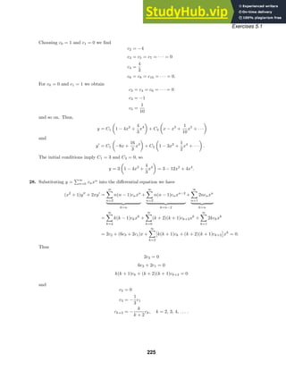

![Exercises 5.1
and so on. Thus, two solutions are
y1 = 1 −
1
6
x3
+
1
120
x5
+ · · · and y2 = x −
1
12
x4
+ · · · .
30. Substituting y =
∞
n=0 cnxn
into the differential equation we have
y
+ ex
y
− y =
∞
n=2
n(n − 1)cnxn−2
+
1 + x +
1
2
x2
+
1
6
x3
+ · · ·
c1 + 2c2x + 3c3x2
+ 4c4x3
+ · · · −
∞
n=0
cnxn
= 2c2 + 6c3x + 12c4x2
+ 20c5x3
+ · · ·
+
c1 + (2c2 + c1)x +
3c3 + 2c2 +
1
2
c1
x2
+ · · ·
− [c0 + c1x + c2x2
+ · · ·]
= (2c2 + c1 − c0) + (6c3 + 2c2)x +
12c4 + 3c3 + c2 +
1
2
c1
x2
+ · · · = 0.
Thus
2c2 + c1 − c0 = 0
6c3 + 2c2 = 0
12c4 + 3c3 + c2 +
1
2
c1 = 0
and
c2 =
1
2
c0 −
1
2
c1
c3 = −
1
3
c2
c4 = −
1
4
c3 +
1
12
c2 −
1
24
c1.
Choosing c0 = 1 and c1 = 0 we find
c2 =
1
2
, c3 = −
1
6
, c4 = 0
and so on. For c0 = 0 and c1 = 1 we obtain
c2 = −
1
2
, c3 =
1
6
, c4 = −
1
24
and so on. Thus, two solutions are
y1 = 1 +
1
2
x2
−
1
6
x3
+ · · · and y2 = x −
1
2
x2
+
1
6
x3
−
1
24
x4
+ · · · .
31. Substituting y =
∞
n=0 cnxn
into the first differential equation leads to
y
− xy =
∞
n=2
n(n − 1)cnxn−2
k=n−2
−
∞
n=0
cnxn+1
k=n+1
=
∞
k=0
(k + 2)(k + 1)ck+2xk
−
∞
k=1
ck−1xk
= 2c2 +
∞
k=1
[(k + 2)(k + 1)ck+2 − ck−1]xk
= 1.
227](https://image.slidesharecdn.com/advancedengineeringmathematicssolutionsmanual-230807162553-1916df96/85/Advanced-Engineering-Mathematics-Solutions-Manual-pdf-227-320.jpg)
![-4 -2 2 4 x
-4
-2
2
4
y
N=2
-4 -2 2 4 x
-4
-2
2
4
y
N=4
-4 -2 2 4 x
-4
-2
2
4
y
N=6
-4 -2 2 4 x
-4
-2
2
4
y
N=8
-4 -2 2 4 x
-4
-2
2
4
y
N=10
-4 -2 2 4 x
-4
-2
2
4
y
N=2
-4 -2 2 4 x
-4
-2
2
4
y
N=4
-4 -2 2 4 x
-4
-2
2
4
y
N=6
-4 -2 2 4 x
-4
-2
2
4
y
N=8
-4 -2 2 4 x
-4
-2
2
4
y
N=10
-4 -2 2 4 x
-4
-2
2
4
y1
-4 -2 2 4 x
-4
-2
2
4
y2
Exercises 5.1
c2 = −
1
2
c3 = c5 = c7 = · · · = 0
c4 = −
1
4
−
1
2
=
1
22 · 2
c6 = −
1
6
1
22 · 2
= −
1
23 · 3!
and so on. For c0 = 0 and c1 = 1 we obtain
c2 = c4 = c6 = · · · = 0
c3 = −
1
3
= −
2
3!
c5 = −
1
5
−
1
3
=
1
5 · 3
=
4 · 2
5!
c7 = −
1
7
4 · 2
5!
= −
6 · 4 · 2
7!
and so on. Thus, two solutions are
y1 =
∞
k=0
(−1)k
2k · k!
x2k
and y2 =
∞
k=0
(−1)k
2k
k!
(2k + 1)!
x2k+1
.
(b) For y1, S3 = S2 and S5 = S4, so we plot S2, S4, S6, S8, and S10.
For y2, S3 = S4 and S5 = S6, so we plot S2, S4, S6, S8, and S10.
(c) The graphs of y1 and y2 obtained from a numerical
solver are shown. We see that the partial sum repre-
sentations indicate the even and odd natures of the so-
lution, but don’t really give a very accurate represen-
tation of the true solution. Increasing N to about 20
gives a much more accurate representation on [−4, 4].
230](https://image.slidesharecdn.com/advancedengineeringmathematicssolutionsmanual-230807162553-1916df96/85/Advanced-Engineering-Mathematics-Solutions-Manual-pdf-230-320.jpg)

![Exercises 5.2
12. Writing the differential equation in the form
y
+
x + 3
x
y
+ 7xy = 0
we see that x0 = 0 is a regular singular point. Multiplying by x2
, the differential equation can be put in the
form
x2
y
+ x(x + 3)y
+ 7x3
y = 0.
We identify p(x) = x + 3 and q(x) = 7x3
.
13. We identify P(x) = 5/3x + 1 and Q(x) = −1/3x2
, so that p(x) = xP(x) = 5
3 + x and q(x) = x2
Q(x) = −1
3 .
Then a0 = 5
3 , b0 = −1
3 , and the indicial equation is
r(r − 1) +
5
3
r −
1
3
= r2
+
2
3
r −
1
3
=
1
3
(3r2
+ 2r − 1) =
1
3
(3r − 1)(r + 1) = 0.
The indicial roots are 1
3 and −1. Since these do not differ by an integer we expect to find two series solutions
using the method of Frobenius.
14. We identify P(x) = 1/x and Q(x) = 10/x, so that p(x) = xP(x) = 1 and q(x) = x2
Q(x) = 10x. Then a0 = 1,
b0 = 0, and the indicial equation is
r(r − 1) + r = r2
= 0.
The indicial roots are 0 and 0. Since these are equal, we expect the method of Frobenius to yield a single series
solution.
15. Substituting y =
∞
n=0 cnxn+r
into the differential equation and collecting terms, we obtain
2xy
− y
+ 2y = 2r2
− 3r c0xr−1
+
∞
k=1
[2(k + r − 1)(k + r)ck − (k + r)ck + 2ck−1]xk+r−1
= 0,
which implies
2r2
− 3r = r(2r − 3) = 0
and
(k + r)(2k + 2r − 3)ck + 2ck−1 = 0.
The indicial roots are r = 0 and r = 3/2. For r = 0 the recurrence relation is
ck = −
2ck−1
k(2k − 3)
, k = 1, 2, 3, . . . ,
and
c1 = 2c0, c2 = −2c0, c3 =
4
9
c0.
For r = 3/2 the recurrence relation is
ck = −
2ck−1
(2k + 3)k
, k = 1, 2, 3, . . . ,
and
c1 = −
2
5
c0, c2 =
2
35
c0, c3 = −
4
945
c0.
The general solution on (0, ∞) is
y = C1
1 + 2x − 2x2
+
4
9
x3
+ · · ·
+ C2x3/2
1 −
2
5
x +
2
35
x2
−
4
945
x3
+ · · ·
.
233](https://image.slidesharecdn.com/advancedengineeringmathematicssolutionsmanual-230807162553-1916df96/85/Advanced-Engineering-Mathematics-Solutions-Manual-pdf-233-320.jpg)
![Exercises 5.2
16. Substituting y =
∞
n=0 cnxn+r
into the differential equation and collecting terms, we obtain
2xy
+ 5y
+ xy = 2r2
+ 3r c0xr−1
+ 2r2
+ 7r + 5 c1xr
+
∞
k=2
[2(k + r)(k + r − 1)ck + 5(k + r)ck + ck−2]xk+r−1
= 0,
which implies
2r2
+ 3r = r(2r + 3) = 0,
2r2
+ 7r + 5 c1 = 0,
and
(k + r)(2k + 2r + 3)ck + ck−2 = 0.
The indicial roots are r = −3/2 and r = 0, so c1 = 0 . For r = −3/2 the recurrence relation is
ck = −
ck−2
(2k − 3)k
, k = 2, 3, 4, . . . ,
and
c2 = −
1
2
c0, c3 = 0, c4 =
1
40
c0.
For r = 0 the recurrence relation is
ck = −
ck−2
k(2k + 3)
, k = 2, 3, 4, . . . ,
and
c2 = −
1
14
c0, c3 = 0, c4 =
1
616
c0.
The general solution on (0, ∞) is
y = C1x−3/2
1 −
1
2
x2
+
1
40
x4
+ · · ·
+ C2
1 −
1
14
x2
+
1
616
x4
+ · · ·
.
17. Substituting y =
∞
n=0 cnxn+r
into the differential equation and collecting terms, we obtain
4xy
+
1
2
y
+ y =
4r2
−
7
2
r
c0xr−1
+
∞
k=1
4(k + r)(k + r − 1)ck +
1
2
(k + r)ck + ck−1
xk+r−1
= 0,
which implies
4r2
−
7
2
r = r
4r −
7
2
= 0
and
1
2
(k + r)(8k + 8r − 7)ck + ck−1 = 0.
The indicial roots are r = 0 and r = 7/8. For r = 0 the recurrence relation is
ck = −
2ck−1
k(8k − 7)
, k = 1, 2, 3, . . . ,
and
c1 = −2c0, c2 =
2
9
c0, c3 = −
4
459
c0.
234](https://image.slidesharecdn.com/advancedengineeringmathematicssolutionsmanual-230807162553-1916df96/85/Advanced-Engineering-Mathematics-Solutions-Manual-pdf-234-320.jpg)
![Exercises 5.2
For r = 7/8 the recurrence relation is
ck = −
2ck−1
(8k + 7)k
, k = 1, 2, 3, . . . ,
and
c1 = −
2
15
c0, c2 =
2
345
c0, c3 = −
4
32,085
c0 .
The general solution on (0, ∞) is
y = C1
1 − 2x +
2
9
x2
−
4
459
x3
+ · · ·
+ C2x7/8
1 −
2
15
x +
2
345
x2
−
4
32,085
x3
+ · · ·
.
18. Substituting y =
∞
n=0 cnxn+r
into the differential equation and collecting terms, we obtain
2x2
y
− xy
+ x2
+ 1 y = 2r2
− 3r + 1 c0xr
+ 2r2
+ r c1xr+1
+
∞
k=2
[2(k + r)(k + r − 1)ck − (k + r)ck + ck + ck−2]xk+r
= 0,
which implies
2r2
− 3r + 1 = (2r − 1)(r − 1) = 0,
2r2
+ r c1 = 0,
and
[(k + r)(2k + 2r − 3) + 1]ck + ck−2 = 0.
The indicial roots are r = 1/2 and r = 1, so c1 = 0. For r = 1/2 the recurrence relation is
ck = −
ck−2
k(2k − 1)
, k = 2, 3, 4, . . . ,
and
c2 = −
1
6
c0, c3 = 0, c4 =
1
168
c0.
For r = 1 the recurrence relation is
ck = −
ck−2
k(2k + 1)
, k = 2, 3, 4, . . . ,
and
c2 = −
1
10
c0, c3 = 0, c4 =
1
360
c0.
The general solution on (0, ∞) is
y = C1x1/2
1 −
1
6
x2
+
1
168
x4
+ · · ·
+ C2x
1 −
1
10
x2
+
1
360
x4
+ · · ·
.
19. Substituting y =
∞
n=0 cnxn+r
into the differential equation and collecting terms, we obtain
3xy
+ (2 − x)y
− y = 3r2
− r c0xr−1
+
∞
k=1
[3(k + r − 1)(k + r)ck + 2(k + r)ck − (k + r)ck−1]xk+r−1
= 0,
235](https://image.slidesharecdn.com/advancedengineeringmathematicssolutionsmanual-230807162553-1916df96/85/Advanced-Engineering-Mathematics-Solutions-Manual-pdf-235-320.jpg)

![Exercises 5.2
21. Substituting y =
∞
n=0 cnxn+r
into the differential equation and collecting terms, we obtain
2xy
− (3 + 2x)y
+ y = 2r2
− 5r c0xr−1
+
∞
k=1
[2(k + r)(k + r − 1)ck
− 3(k + r)ck − 2(k + r − 1)ck−1 + ck−1]xk+r−1
= 0,
which implies
2r2
− 5r = r(2r − 5) = 0
and
(k + r)(2k + 2r − 5)ck − (2k + 2r − 3)ck−1 = 0.
The indicial roots are r = 0 and r = 5/2. For r = 0 the recurrence relation is
ck =
(2k − 3)ck−1
k(2k − 5)
, k = 1, 2, 3, . . . ,
and
c1 =
1
3
c0, c2 = −
1
6
c0, c3 = −
1
6
c0.
For r = 5/2 the recurrence relation is
ck =
2(k + 1)ck−1
k(2k + 5)
, k = 1, 2, 3, . . . ,
and
c1 =
4
7
c0, c2 =
4
21
c0, c3 =
32
693
c0.
The general solution on (0, ∞) is
y = C1
1 +
1
3
x −
1
6
x2
−
1
6
x3
+ · · ·
+ C2x5/2
1 +
4
7
x +
4
21
x2
+
32
693
x3
+ · · ·
.
22. Substituting y =
∞
n=0 cnxn+r
into the differential equation and collecting terms, we obtain
x2
y
+ xy
+
x2
−
4
9
y =
r2
−
4
9
c0xr
+
r2
+ 2r +
5
9
c1xr+1
+
∞
k=2
(k + r)(k + r − 1)ck + (k + r)ck −
4
9
ck + ck−2
xk+r
= 0,
which implies
r2
−
4
9
=
r +
2
3
r −
2
3
= 0,
r2
+ 2r +
5
9
c1 = 0,
and
(k + r)2
−
4
9
ck + ck−2 = 0.
The indicial roots are r = −2/3 and r = 2/3, so c1 = 0. For r = −2/3 the recurrence relation is
ck = −
9ck−2
3k(3k − 4)
, k = 2, 3, 4, . . . ,
237](https://image.slidesharecdn.com/advancedengineeringmathematicssolutionsmanual-230807162553-1916df96/85/Advanced-Engineering-Mathematics-Solutions-Manual-pdf-237-320.jpg)
![Exercises 5.2
and
c2 = −
3
4
c0, c3 = 0, c4 =
9
128
c0.
For r = 2/3 the recurrence relation is
ck = −
9ck−2
3k(3k + 4)
, k = 2, 3, 4, . . . ,
and
c2 = −
3
20
c0, c3 = 0, c4 =
9
1,280
c0.
The general solution on (0, ∞) is
y = C1x−2/3
1 −
3
4
x2
+
9
128
x4
+ · · ·
+ C2x2/3
1 −
3
20
x2
+
9
1,280
x4
+ · · ·
.
23. Substituting y =
∞
n=0 cnxn+r
into the differential equation and collecting terms, we obtain
9x2
y
+ 9x2
y
+ 2y = 9r2
− 9r + 2 c0xr
+
∞
k=1
[9(k + r)(k + r − 1)ck + 2ck + 9(k + r − 1)ck−1]xk+r
= 0,
which implies
9r2
− 9r + 2 = (3r − 1)(3r − 2) = 0
and
[9(k + r)(k + r − 1) + 2]ck + 9(k + r − 1)ck−1 = 0.
The indicial roots are r = 1/3 and r = 2/3. For r = 1/3 the recurrence relation is
ck = −
(3k − 2)ck−1
k(3k − 1)
, k = 1, 2, 3, . . . ,
and
c1 = −
1
2
c0, c2 =
1
5
c0, c3 = −
7
120
c0.
For r = 2/3 the recurrence relation is
ck = −
(3k − 1)ck−1
k(3k + 1)
, k = 1, 2, 3, . . . ,
and
c1 = −
1
2
c0, c2 =
5
28
c0, c3 = −
1
21
c0.
The general solution on (0, ∞) is
y = C1x1/3
1 −
1
2
x +
1
5
x2
−
7
120
x3
+ · · ·
+ C2x2/3
1 −
1
2
x +
5
28
x2
−
1
21
x3
+ · · ·
.
24. Substituting y =
∞
n=0 cnxn+r
into the differential equation and collecting terms, we obtain
2x2
y
+ 3xy
+ (2x − 1)y = 2r2
+ r − 1 c0xr
+
∞
k=1
[2(k + r)(k + r − 1)ck + 3(k + r)ck − ck + 2ck−1]xk+r
= 0,
238](https://image.slidesharecdn.com/advancedengineeringmathematicssolutionsmanual-230807162553-1916df96/85/Advanced-Engineering-Mathematics-Solutions-Manual-pdf-238-320.jpg)
![Exercises 5.2
which implies
2r2
+ r − 1 = (2r − 1)(r + 1) = 0
and
[(k + r)(2k + 2r + 1) − 1]ck + 2ck−1 = 0.
The indicial roots are r = −1 and r = 1/2. For r = −1 the recurrence relation is
ck = −
2ck−1
k(2k − 3)
, k = 1, 2, 3, . . . ,
and
c1 = 2c0, c2 = −2c0, c3 =
4
9
c0.
For r = 1/2 the recurrence relation is
ck = −
2ck−1
k(2k + 3)
, k = 1, 2, 3, . . . ,
and
c1 = −
2
5
c0, c2 =
2
35
c0, c3 = −
4
945
c0.
The general solution on (0, ∞) is
y = C1x−1
1 + 2x − 2x2
+
4
9
x3
+ · · ·
+ C2x1/2
1 −
2
5
x +
2
35
x2
−
4
945
x3
+ · · ·
.
25. Substituting y =
∞
n=0 cnxn+r
into the differential equation and collecting terms, we obtain
xy
+ 2y
− xy = r2
+ r c0xr−1
+ r2
+ 3r + 2 c1xr
+
∞
k=2
[(k + r)(k + r − 1)ck + 2(k + r)ck − ck−2]xk+r−1
= 0,
which implies
r2
+ r = r(r + 1) = 0,
r2
+ 3r + 2 c1 = 0,
and
(k + r)(k + r + 1)ck − ck−2 = 0.
The indicial roots are r1 = 0 and r2 = −1, so c1 = 0. For r1 = 0 the recurrence relation is
ck =
ck−2
k(k + 1)
, k = 2, 3, 4, . . . ,
and
c2 =
1
3!
c0
c3 = c5 = c7 = · · · = 0
c4 =
1
5!
c0
c2n =
1
(2n + 1)!
c0.
239](https://image.slidesharecdn.com/advancedengineeringmathematicssolutionsmanual-230807162553-1916df96/85/Advanced-Engineering-Mathematics-Solutions-Manual-pdf-239-320.jpg)
![Exercises 5.2
For r2 = −1 the recurrence relation is
ck =
ck−2
k(k − 1)
, k = 2, 3, 4, . . . ,
and
c2 =
1
2!
c0
c3 = c5 = c7 = · · · = 0
c4 =
1
4!
c0
c2n =
1
(2n)!
c0.
The general solution on (0, ∞) is
y = C1
∞
n=0
1
(2n + 1)!
x2n
+ C2x−1
∞
n=0
1
(2n)!
x2n
=
1
x
C1
∞
n=0
1
(2n + 1)!
x2n+1
+ C2
∞
n=0
1
(2n)!
x2n
=
1
x
[C1 sinh x + C2 cosh x].
26. Substituting y =
∞
n=0 cnxn+r
into the differential equation and collecting terms, we obtain
x2
y
+ xy
+
x2
−
1
4
y =
r2
−
1
4
c0xr
+
r2
+ 2r +
3
4
c1xr+1
+
∞
k=2
(k + r)(k + r − 1)ck + (k + r)ck −
1
4
ck + ck−2
xk+r
= 0,
which implies
r2
−
1
4
=
r −
1
2
r +
1
2
= 0,
r2
+ 2r +
3
4
c1 = 0,
and
(k + r)2
−
1
4
ck + ck−2 = 0.
The indicial roots are r1 = 1/2 and r2 = −1/2, so c1 = 0. For r1 = 1/2 the recurrence relation is
ck = −
ck−2
k(k + 1)
, k = 2, 3, 4, . . . ,
and
c2 = −
1
3!
c0
c3 = c5 = c7 = · · · = 0
c4 =
1
5!
c0
c2n =
(−1)n
(2n + 1)!
c0.
240](https://image.slidesharecdn.com/advancedengineeringmathematicssolutionsmanual-230807162553-1916df96/85/Advanced-Engineering-Mathematics-Solutions-Manual-pdf-240-320.jpg)
![Exercises 5.2
For r2 = −1/2 the recurrence relation is
ck = −
ck−2
k(k − 1)
, k = 2, 3, 4, . . . ,
and
c2 = −
1
2!
c0
c3 = c5 = c7 = · · · = 0
c4 =
1
4!
c0
c2n =
(−1)n
(2n)!
c0.
The general solution on (0, ∞) is
y = C1x1/2
∞
n=0
(−1)n
(2n + 1)!
x2n
+ C2x−1/2
∞
n=0
(−1)n
(2n)!
x2n
= C1x−1/2
∞
n=0
(−1)n
(2n + 1)!
x2n+1
+ C2x−1/2
∞
n=0
(−1)n
(2n)!
x2n
= x−1/2
[C1 sin x + C2 cos x].
27. Substituting y =
∞
n=0 cnxn+r
into the differential equation and collecting terms, we obtain
xy
− xy
+ y = r2
− r c0xr−1
+
∞
k=0
[(k + r + 1)(k + r)ck+1 − (k + r)ck + ck]xk+r
= 0
which implies
r2
− r = r(r − 1) = 0
and
(k + r + 1)(k + r)ck+1 − (k + r − 1)ck = 0.
The indicial roots are r1 = 1 and r2 = 0. For r1 = 1 the recurrence relation is
ck+1 =
kck
(k + 2)(k + 1)
, k = 0, 1, 2, . . . ,
and one solution is y1 = c0x. A second solution is
y2 = x
e−
− dx
x2
dx = x
ex
x2
dx = x
1
x2
1 + x +
1
2
x2
+
1
3!
x3
+ · · ·
dx
= x
1
x2
+
1
x
+
1
2
+
1
3!
x +
1
4!
x2
+ · · ·
dx = x
−
1
x
+ ln x +
1
2
x +
1
12
x2
+
1
72
x3
+ · · ·
= x ln x − 1 +
1
2
x2
+
1
12
x3
+
1
72
x4
+ · · · .
The general solution on (0, ∞) is
y = C1x + C2y2(x).
241](https://image.slidesharecdn.com/advancedengineeringmathematicssolutionsmanual-230807162553-1916df96/85/Advanced-Engineering-Mathematics-Solutions-Manual-pdf-241-320.jpg)
![Exercises 5.2
28. Substituting y =
∞
n=0 cnxn+r
into the differential equation and collecting terms, we obtain
y
+
3
x
y
− 2y = r2
+ 2r c0xr−2
+ r2
+ 4r + 3 c1xr−1
+
∞
k=2
[(k + r)(k + r − 1)ck + 3(k + r)ck − 2ck−2]xk+r−2
= 0,
which implies
r2
+ 2r = r(r + 2) = 0
r2
+ 4r + 3 c1 = 0
(k + r)(k + r + 2)ck − 2ck−2 = 0.
The indicial roots are r1 = 0 and r2 = −2, so c1 = 0. For r1 = 0 the recurrence relation is
ck =
2ck−2
k(k + 2)
, k = 2, 3, 4, . . . ,
and
c2 =
1
4
c0
c3 = c5 = c7 = · · · = 0
c4 =
1
48
c0
c6 =
1
1,152
c0.
The result is
y1 = c0
1 +
1
4
x2
+
1
48
x4
+
1
1,152
c6 + · · ·
.
A second solution is
y2 = y1
e−
(3/x)dx
y2
1
dx = y1
dx
x3 1 + 1
4 x2 + 1
48 x4 + · · ·
2
= y1
dx
x3 1 + 1
2 x2 + 5
48 x4 + 7
576 x6 + · · ·
= y1
1
x3
1 −
1
2
x2
+
7
48
x4
+
19
576
x6
+ · · ·
= y1
1
x3
−
1
2x
+
7
48
x −
19
576
x3
+ · · ·
= y1
−
1
2x2
−
1
2
ln x +
7
96
x2
−
19
2,304
x4
+ · · ·
= −
1
2
y1 ln x + y
−
1
2x2
+
7
96
x2
−
19
2,304
x4
+ · · ·
.
The general solution on (0, ∞) is
y = C1y1(x) + C2y2(x).
29. Substituting y =
∞
n=0 cnxn+r
into the differential equation and collecting terms, we obtain
xy
+ (1 − x)y
− y = r2
c0xr−1
+
∞
k=0
[(k + r)(k + r − 1)ck + (k + r)ck − (k + r)ck−1]xk+r−1
= 0,
which implies r2
= 0 and
(k + r)2
ck − (k + r)ck−1 = 0.
242](https://image.slidesharecdn.com/advancedengineeringmathematicssolutionsmanual-230807162553-1916df96/85/Advanced-Engineering-Mathematics-Solutions-Manual-pdf-242-320.jpg)
![Exercises 5.2
The indicial roots are r1 = r2 = 0 and the recurrence relation is
ck =
ck−1
k
, k = 1, 2, 3, . . . .
One solution is
y1 = c0
1 + x +
1
2
x2
+
1
3!
x3
+ · · ·
= c0ex
.
A second solution is
y2 = y1
e−
(1/x−1)dx
e2x
dx = ex
ex
/x
e2x
dx = ex
1
x
e−x
dx
= ex
1
x
1 − x +
1
2
x2
−
1
3!
x3
+ · · ·
dx = ex
1
x
− 1 +
1
2
x −
1
3!
x2
+ · · ·
dx
= ex
ln x − x +
1
2 · 2
x2
−
1
3 · 3!
x3
+ · · ·
= ex
ln x − ex
∞
n=1
(−1)n+1
n · n!
xn
.
The general solution on (0, ∞) is
y = C1ex
+ C2ex
ln x −
∞
n=1
(−1)n+1
n · n!
xn
.
30. Substituting y =
∞
n=0 cnxn+r
into the differential equation and collecting terms, we obtain
xy
+ y
+ y = r2
c0xr−1
+
∞
k=1
[(k + r)(k + r − 1)ck + (k + r)ck + ck−1]xk+r−1
= 0
which implies r2
= 0 and
(k + r)2
ck + ck−1 = 0.
The indicial roots are r1 = r2 = 0 and the recurrence relation is
ck = −
ck−1
k2
, k = 1, 2, 3, . . . .
One solution is
y1 = c0
1 − x +
1
22
x2
−
1
(3!)2
x3
+
1
(4!)2
x4
− · · ·
= c0
∞
n=0
(−1)n
(n!)2
xn
.
A second solution is
y2 = y1
e−
(1/x)dx
y2
1
dx = y1
dx
x 1 − x + 1
4 x2 − 1
36 x3 + · · ·
2
= y1
dx
x 1 − 2x + 3
2 x2 − 5
9 x3 + 35
288 x4 − · · ·
= y1
1
x
1 + 2x +
5
2
x2
+
23
9
x3
+
677
288
x4
+ · · ·
dx
= y1
1
x
+ 2 +
5
2
x +
23
9
x2
+
677
288
x3
+ · · ·
dx
= y1
ln x + 2x +
5
4
x2
+
23
27
x3
+
677
1,152
x4
+ · · ·
= y1 ln x + y1
2x +
5
4
x2
+
23
27
x3
+
677
1,152
x4
+ · · ·
.
243](https://image.slidesharecdn.com/advancedengineeringmathematicssolutionsmanual-230807162553-1916df96/85/Advanced-Engineering-Mathematics-Solutions-Manual-pdf-243-320.jpg)
![Exercises 5.2
Taking c0 = 0 and c7 = 0 we obtain
c1 = c2 = c3 = c4 = c5 = c6 = 0
c8 = −
1
2
c7
c9 =
5
36
c7
c10 = −
1
36
c7.
In this case we obtain the two solutions
y1 = 1 −
1
2
x +
1
10
x2
−
1
120
x3
and y2 = x7
−
1
2
x8
+
5
36
x9
−
1
36
x10
+ · · · .
32. Substituting y =
∞
n=0 cnxn+r
into the differential equation and collecting terms, we obtain
x(x − 1)y
+ 3y
− 2y
= 4r − r2
c0xr−1
+
∞
k=1
[(k + r − 1)(k + r − 12)ck−1 − (k + r)(k + r − 1)ck
+ 3(k + r)ck − 2ck−1]xk+r−1
= 0,
which implies
4r − r2
= r(4 − r) = 0
and
−(k + r)(k + r − 4)ck + [(k + r − 1)(k + r − 2) − 2]ck−1 = 0.
The indicial roots are r1 = 4 and r2 = 0. For r1 = 4 the recurrence relation is
−(k + 4)kck + [(k + 3)(k + 2) − 2]ck−1 = 0
or
ck = (k + 1)ck−1, k = 1, 2, 3, . . . .
Taking c0 = 0 we obtain
c1 = 2c0
c2 = 3!c0
c3 = 4!c0,
and so on. Thus, the indicial root r1 = 4 yields a single solution. For r2 = 0 the recurrence relation is
−k(k − 4)ck + k(k − 3)ck−1 = 0, k = 1, 2, 3, . . . ,
or
−(k − 4)ck + (k − 3)ck−1 = 0, k = 1, 2, 3, . . . .
Then
3c1 − 2c0 = 0
2c2 − c1 = 0
c3 + 0c2 = 0 ⇒ c3 = 0
0c4 + c3 = 0 ⇒ c4 is arbitrary
245](https://image.slidesharecdn.com/advancedengineeringmathematicssolutionsmanual-230807162553-1916df96/85/Advanced-Engineering-Mathematics-Solutions-Manual-pdf-245-320.jpg)
![Exercises 5.2
and
ck =
(k − 3)ck−1
c − 4
, k = 5, 6, 7, . . . .
Taking c0 = 0 and c4 = 0 we obtain
c1 =
2
3
c0
c2 =
1
3
c0
c3 = c4 = c5 = · · · = 0.
Taking c0 = 0 and c4 = 0 we obtain
c1 = c2 = c3 = 0
c5 = 2c4
c6 = 3c4
c7 = 4c4.
In this case we obtain the two solutions
y1 = 1 +
2
3
x +
1
3
x2
and y2 = x4
+ 2x5
+ 3x6
+ 4x7
+ · · · .
33. (a) From t = 1/x we have dt/dx = −1/x2
= −t2
. Then
dy
dx
=
dy
dt
dt
dx
= −t2 dy
dt
and
d2
y
dx2
=
d
dx
dy
dx
=
d
dx
−t2 dy
dt
= −t2 d2
y
dt2
dt
dx
−
dy
dt
2t
dt
dx
= t4 d2
y
dt2
+ 2t3 dy
dt
.
Now
x4 d2
y
dx2
+ λy =
1
t4
t4 d2
y
dt2
+ 2t3 dy
dt
+ λy =
d2
y
dt2
+
2
t
dy
dt
+ λy = 0
becomes
t
d2
y
dt2
+ 2
dy
dt
+ λty = 0.
(b) Substituting y =
∞
n=0 cntn+r
into the differential equation and collecting terms, we obtain
t
d2
y
dt2
+ 2
dy
dt
+ λty = (r2
+ r)c0tr−1
+ (r2
+ 3r + 2)c1tr
+
∞
k=2
[(k + r)(k + r − 1)ck + 2(k + r)ck + λck−2]tk+r−1
= 0,
which implies
r2
+ r = r(r + 1) = 0,
r2
+ 3r + 2 c1 = 0,
and
(k + r)(k + r + 1)ck + λck−2 = 0.
The indicial roots are r1 = 0 and r2 = −1, so c1 = 0. For r1 = 0 the recurrence relation is
ck = −
λck−2
k(k + 1)
, k = 2, 3, 4, . . . ,
246](https://image.slidesharecdn.com/advancedengineeringmathematicssolutionsmanual-230807162553-1916df96/85/Advanced-Engineering-Mathematics-Solutions-Manual-pdf-246-320.jpg)
![Exercises 5.2
and
c2 = −
λ
3!
c0
c3 = c5 = c7 = · · · = 0
c4 =
λ2
5!
c0
c2n = (−1)n λn
(2n + 1)!
c0.
For r2 = −1 the recurrence relation is
ck = −
λck−2
k(k − 1)
, k = 2, 3, 4, . . . ,
and
c2 = −
λ
2!
c0
c3 = c5 = c7 = · · · = 0
c4 =
λ2
4!
c0
c2n = (−1)n λn
(2n)!
c0.
The general solution on (0, ∞) is
y(t) = C1
∞
n=0
(−1)n
(2n + 1)!
(
√
λ t)2n
+ C2t−1
∞
n=0
(−1)n
(2n)!
(
√
λ t)2n
=
1
t
C1
∞
n=0
(−1)n
(2n + 1)!
(
√
λ t)2n+1
+ C2
∞
n=0
(−1)n
(2n)!
(
√
λ t)2n
=
1
t
[C1 sin
√
λ t + C2 cos
√
λ t ].
(c) Using t = 1/x, the solution of the original equation is
y(x)C1x sin
√
λ
x
+ C2x cos
√
λ
x
.
34. (a) From the boundary conditions y(a) = 0, y(b) = 0 we find
C1 sin
√
λ
a
+ C2 cos
√
λ
a
= 0
C1 sin
√
λ
b
+ C2 cos
√
λ
b
= 0.
Since this is a homogeneous system of linear equations, it will have nontrivial solutions if
sin
√
λ
a
cos
√
λ
a
sin
√
λ
b
cos
√
λ
b
= sin
√
λ
a
cos
√
λ
b
− cos
√
λ
a
sin
√
λ
b
= sin
√
λ
a
−
√
λ
b
= sin
√
λ
b − a
ab
= 0.
This will be the case if
√
λ
b − a
ab
= nπ or
√
λ =
nλab
b − a
=
nλab
L
, n = 1, 2, . . . ,
247](https://image.slidesharecdn.com/advancedengineeringmathematicssolutionsmanual-230807162553-1916df96/85/Advanced-Engineering-Mathematics-Solutions-Manual-pdf-247-320.jpg)
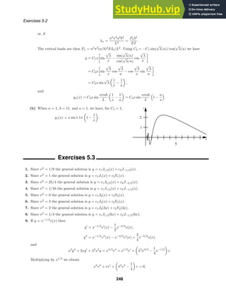
![Exercises 5.3
whose solution is v = c1J1/2(λx) + c2J−1/2(λx). Then y = c1x−1/2
J1/2(λx) + c2x−1/2
J−1/2(λx).
10. From y = xn
Jn(x) we find
y
= xn
J
n + nxn−1
Jn and y
= xn
J
n + 2nxn−1
J
n + n(n − 1)xn−2
Jn.
Substituting into the differential equation, we have
xn+1
J
n + 2nxn
J
n + n(n − 1)xn−1
Jn + (1 − 2n)(xn
J
n + nxn−1
Jn) + xn+1
Jn
= xn+1
J
n + (2n + 1 − 2n)xn
J
n + (n2
− n + n − 2n2
)xn−1
Jn + xn+1
Jn
= xn+1
[x2
J
n + xJ
n − n2
Jn + x2
Jn]
= xn+1
[x2
J
n + xJ
n + (x2
− n2
)Jn]
= xn−1
· 0 (since Jn is a solution of Bessel’s equation)
= 0.
Therefore, xn
Jn is a solution of the original equation.
11. From y = x−n
Jn we find
y
= x−n
J
n − nx−n−1
Jn and y
= x−n
J
n − 2nx−n−1
J
n + n(n + 1)x−n−2
Jn.
Substituting into the differential equation, we have
xy
+ (1 + 2n)y
+ xy = x−n−1
x2
J
n + xJ
n + x2
− n2
Jn
= x−n−1
· 0 (since Jn is a solution of Bessel’s equation)
= 0.
Therefore, x−n
Jn is a solution of the original equation.
12. From y =
√
x Jν(λx) we find
y
= λ
√
x J
ν(λx) +
1
2
x−1/2
Jν(λx)
and
y
= λ2
√
x J
ν (λx) + λx−1/2
J
ν(λx) −
1
4
x−3/2
Jν(λx).
Substituting into the differential equation, we have
x2
y
+
λ2
x2
− ν2
+
1
4
y =
√
x λ2
x2
J
ν (λx) + λxJ
ν(λx) + λ2
x2
− ν2
Jν(λx)
=
√
x · 0 (since Jn is a solution of Bessel’s equation)
= 0.
Therefore,
√
x Jν(λx) is a solution of the original equation.
13. From Problem 10 with n = 1/2 we find y = x1/2
J1/2(x). From Problem 11 with n = −1/2 we find y =
x1/2
J−1/2(x).
14. From Problem 10 with n = 1 we find y = xJ1(x). From Problem 11 with n = −1 we find y = xJ−1(x) = −xJ1(x).
15. From Problem 10 with n = −1 we find y = x−1
J−1(x). From Problem 11 with n = 1 we find y = x−1
J1(x) =
−x−1
J−1(x).
16. From Problem 12 with λ = 2 and ν = 0 we find y =
√
x J0(2x).
17. From Problem 12 with λ = 1 and ν = ±3/2 we find y =
√
x J3/2(x) and y =
√
x J−3/2(x).
249](https://image.slidesharecdn.com/advancedengineeringmathematicssolutionsmanual-230807162553-1916df96/85/Advanced-Engineering-Mathematics-Solutions-Manual-pdf-249-320.jpg)
![Exercises 5.3
18. From Problem 10 with n = 3 we find y = x3
J3(x). From Problem 11 with n = −3 we find y = x3
J−3(x) =
−x3
J3(x).
19. (a) The recurrence relation follows from
−νJν(x) + xJν−1(x) = −
∞
n=0
(−1)n
ν
n!Γ(1 + ν + n)
x
2
2n+ν
+ x
∞
n=0
(−1)n
n!Γ(ν + n)
x
2
2n+ν−1
= −
∞
n=0
(−1)n
ν
n!Γ(1 + ν + n)
x
2
2n+ν
+
∞
n=0
(−1)n
(ν + n)
n!Γ(1 + ν + n)
· 2
x
2
x
2
2n+ν−1
=
∞
n=0
(−1)n
(2n + ν)
n!Γ(1 + ν + n)
x
2
2n+ν
= xJ
ν(x).
(b) The formula in part (a) is a linear first-order differential equation in Jν(x). An integrating factor for this
equation is xν
, so
d
dx
[xν
Jν(x)] = xν
Jν−1(x).
20. Subtracting the formula in part (a) of Problem 19 from the formula in Example 4 we obtain
0 = 2νJν(x) − xJν+1(x) − xJν−1(x) or 2νJν(x) = xJν+1(x) + xJν−1(x).
21. Letting ν = 1 in (15) we have
xJ0(x) =
d
dx
[xJ1(x)] so
x
0
rJ0(r) dr = rJ1(r)
r=x
r=0
= xJ1(x).
22. From (14) we obtain J
0(x) = −J1(x), and from (15) we obtain J
0(x) = J−1(x). Thus J
0(x) = J−1(x) = −J1(x).
23. Since
Γ
1 −
1
2
+ n
=
(2n − 1)!
(n − 1)!22n−1
we obtain
J−1/2(x) =
∞
n=0
(−1)n
21/2
x−1/2
2n(2n − 1)!
√
π
x2n
=
2
πx
cos x.
24. (a) By Problem 20, with ν = 1/2, we obtain J1/2(x) = xJ3/2(x) + xJ−1/2(x) so that
J3/2(x) =
2
πx
sin x
x
− cos x
;
with ν = −1/2 we obtain −J−1/2(x) = xJ1/2(x) + xJ−3/2(x) so that
J−3/2(x) = −
2
πx
cos x
x
+ sin x
;
and with ν = 3/2 we obtain 3J3/2(x) = xJ5/2(x) + xJ1/2(x) so that
J5/2(x) =
2
πx
3 sin x
x2
−
3 cos x
x
− sin x
.
250](https://image.slidesharecdn.com/advancedengineeringmathematicssolutionsmanual-230807162553-1916df96/85/Advanced-Engineering-Mathematics-Solutions-Manual-pdf-250-320.jpg)
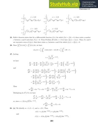
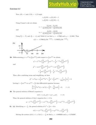
![t
x
50 100 150 200
−1
1
Exercises 5.3
(b)
32. (a) Letting t = L − x, the boundary-value problem becomes
d2
θ
dt2
+ α2
tθ = 0, θ
(0) = 0, θ(L) = 0,
where α2
= δg/EI. This is Airy’s differential equation, so by Problem 30 its solution is
y = c1t1/2
J1/3
2
3
αt3/2
+ c2t1/2
J−1/3
2
3
αt3/2
= c1θ1(t) + c2θ2(t).
(b) Looking at the series forms of θ1 and θ2 we see that θ
1(0) = 0, while θ
2(0) = 0. Thus, the boundary
condition θ
(0) = 0 implies c1 = 0, and so
θ(t) = c2
√
t J−1/3
2
3
αt3/2
.
From θ(L) = 0 we have
c2
√
L J−1/3
2
3
αL3/2
= 0,
so either c2 = 0, in which case θ(t) = 0, or J−1/3(2
3 αL3/2
) = 0. The column will just start to bend when
L is the length corresponding to the smallest positive zero of J−1/3. Using Mathematica, the first positive
root of J−1/3(x) is x1 ≈ 1.86635. Thus 2
3 αL3/2
= 1.86635 implies
L =
3(1.86635)
2α
2/3
=
9EI
4δg
(1.86635)2
1/3
=
9(2.6 × 10⁷
)π(0.05)4
/4
4(0.28)π(0.05)2
(1.86635)2
1/3
≈ 76.9 in.
33. Setting y =
√
x J1(2
√
x ) and differentiating we obtain
y
=
√
x J
1(2
√
x )
2
2
√
x
+
1
2
√
x
J1(2
√
x ) = J
1(2
√
x ) +
1
2
√
x
J1(2
√
x )
and
y
= J
1 (2
√
x )
2
2
√
x
+
1
2
√
x
J
1(2
√
x )
2
2
√
x
−
1
4x3/2
J1(2
√
x )
=
1
√
x
J
1 (2
√
x ) +
1
2x
J
1(2
√
x ) −
1
4x3/2
J1(2
√
x ).
Substituting into the differential equation and letting t = 2
√
x we have
xy
+ y =
√
x J
1 (2
√
x ) +
1
2
J
1(2
√
x ) −
1
4
√
x
J1(2
√
x ) +
√
x J1(2
√
x )
=
1
√
x
xJ
1 (2
√
x ) +
√
x
2
J
1(2
√
x ) +
x −
1
4
J1(2
√
x )
=
2
t
t2
4
J
1 (t) +
t
4
J
1(t) +
t2
4
−
1
4
J1(t)
=
1
2t
[ t2
J
1 (t) + tJ
1(t) + (t2
− 1)J1(t)].
253](https://image.slidesharecdn.com/advancedengineeringmathematicssolutionsmanual-230807162553-1916df96/85/Advanced-Engineering-Mathematics-Solutions-Manual-pdf-253-320.jpg)
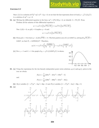

![Chapter 5 Review Exercises
Chapter 5 Review Exercises
1. The interval of convergence is centered at 4. Since the series converges at −2, it converges at least on the interval
[−2, 10). Since it diverges at 13, it converges at most on the interval [−5, 13). Thus at 10 it might converge; at
7 it does converge; at −7 it does not converge: and at 11 it might converge.
2. We have
f(x) =
sin x
cos x
=
x −
x3
6
+
x5
120
− · · ·
1 −
x2
2
+
x4
24
− · · ·
= x +
x3
3
+
2x5
15
+ · · · .
3. Solving x2
− 2x + 10 = 0 we obtain x = 1 ±
√
11 , which are singular points. Thus, the minimum radius of
convergence is |1 −
√
11 | =
√
11 − 1.
4. Setting 1 − sin x = 0 we see the singular points closest to 0 are −3π/2 and π/2. Thus, the minimum radius of
convergence is π/2.
5. The differential equation (x3
−x2
)y
+y
+y = 0 has a regular singular point at x = 1 and an irregular singular
point at x = 1.
6. The differential equation (x − 1)(x + 3)y
+ y = 0 has regular singular points at x = 1 and x = −3.
7. Substituting y =
∞
n=0 cnxn+r
into the differential equation we obtain
2xy
+ y
+ y = 2r2
− r c0xr−1
+
∞
k=1
[2(k + r)(k + r − 1)ck + (k + r)ck + ck−1]xk+r−1
= 0
which implies
2r2
− r = r(2r − 1) = 0
and
(k + r)(2k + 2r − 1)ck + ck−1 = 0.
The indicial roots are r = 0 and r = 1/2. For r = 0 the recurrence relation is
ck = −
ck−1
k(2k − 1)
, k = 1, 2, 3, . . . ,
so
c1 = −c0, c2 =
1
6
c0, c3 = −
1
90
c0.
For r = 1/2 the recurrence relation is
ck = −
ck−1
k(2k + 1)
, k = 1, 2, 3, . . . ,
so
c1 = −
1
3
c0, c2 =
1
30
c0, c3 = −
1
630
c0.
Two linearly independent solutions are
y1 = C1
1 − x +
1
6
x2
−
1
90
x3
+ · · ·
and
y2 = C2x1/2
1 −
1
3
x +
1
30
x2
−
1
630
x3
+ · · ·
.
256](https://image.slidesharecdn.com/advancedengineeringmathematicssolutionsmanual-230807162553-1916df96/85/Advanced-Engineering-Mathematics-Solutions-Manual-pdf-256-320.jpg)
![Chapter 5 Review Exercises
8. Substituting y =
∞
n=0 cnxn
into the differential equation we have
y
− xy
− y =
∞
n=2
n(n − 1)cnxn−2
k=n−2
−
∞
n=1
ncnxn
k=n
−
∞
n=0
cnxn
k=n
=
∞
k=0
(k + 2)(k + 1)ck+2xk
−
∞
k=1
kckxk
−
∞
k=0
ckxk
= 2c2 − c0 +
∞
k=1
[(k + 2)(k + 1)ck+2 − (k + 1)ck]xk
= 0.
Thus
2c2 − c0 = 0
(k + 2)(k + 1)ck+2 − (k + 1)ck = 0
and
c2 =
1
2
c0
ck+2 =
1
k + 2
ck, k = 1, 2, 3, . . . .
Choosing c0 = 1 and c1 = 0 we find
c2 =
1
2
c3 = c5 = c7 = · · · = 0
c4 =
1
8
c6 =
1
48
and so on. For c0 = 0 and c1 = 1 we obtain
c2 = c4 = c6 = · · · = 0
c3 =
1
3
c5 =
1
15
c7 =
1
105
and so on. Thus, two solutions are
y1 = 1 +
1
2
x2
+
1
8
x4
+
1
48
x6
+ · · ·
and
y2 = x +
1
3
x3
+
1
15
x5
+
1
105
x7
+ · · · .
9. Substituting y =
∞
n=0 cnxn
into the differential equation we obtain
(x − 1)y
+ 3y = (−2c2 + 3c0) +
∞
k=3
(k − 1)(k − 2)ck−1 − k(k − 1)ck + 3ck−2]xk−2
= 0
which implies c2 = 3c0/2 and
ck =
(k − 1)(k − 2)ck−1 + 3ck−2
k(k − 1)
, k = 3, 4, 5, . . . .
257](https://image.slidesharecdn.com/advancedengineeringmathematicssolutionsmanual-230807162553-1916df96/85/Advanced-Engineering-Mathematics-Solutions-Manual-pdf-257-320.jpg)
![Chapter 5 Review Exercises
Choosing c0 = 1 and c1 = 0 we find
c2 =
3
2
, c3 =
1
2
, c4 =
5
8
and so on. For c0 = 0 and c1 = 1 we obtain
c2 = 0, c3 =
1
2
, c4 =
1
4
and so on. Thus, two solutions are
y1 = C1
1 +
3
2
x2
+
1
2
x3
+
5
8
x4
+ · · ·
and
y2 = C2
x +
1
2
x3
+
1
4
x4
+ · · ·
.
10. Substituting y =
∞
n=0 cnxn
into the differential equation we obtain
y
− x2
y
+ xy = 2c2 + (6c3 + c0)x +
∞
k=1
[(k + 3)(k + 2)ck+3 − (k − 1)ck]xk+1
= 0
which implies c2 = 0, c3 = −c0/6, and
ck+3 =
k − 1
(k + 3)(k + 2)
ck, k = 1, 2, 3, . . . .
Choosing c0 = 1 and c1 = 0 we find
c3 = −
1
6
c4 = c7 = c10 = · · · = 0
c5 = c8 = c11 = · · · = 0
c6 = −
1
90
and so on. For c0 = 0 and c1 = 1 we obtain
c3 = c6 = c9 = · · · = 0
c4 = c7 = c10 = · · · = 0
c5 = c8 = c11 = · · · = 0
and so on. Thus, two solutions are
y1 = c0
1 −
1
6
x3
−
1
90
x6
− · · ·
and y2 = c1x.
11. Substituting y =
∞
n=0 cnxn+r
into the differential equation and collecting terms, we obtain
xy
+ (x − 6)y
− 3y = (r2
− 7r)c0xr−1
+
∞
k=1
(k + r)(k + r − 1)ck + (k + r − 1)ck−1
− 6(k + r)ck − 3ck−1 xk+r−1
= 0,
which implies
r2
− 7r = r(r − 7) = 0
and
(k + r)(k + r − 7)ck + (k + r − 4)ck−1 = 0.
258](https://image.slidesharecdn.com/advancedengineeringmathematicssolutionsmanual-230807162553-1916df96/85/Advanced-Engineering-Mathematics-Solutions-Manual-pdf-258-320.jpg)
![Chapter 5 Review Exercises
The indicial roots are r1 = 7 and r2 = 0. For r2 = 0 the recurrence relation is
k(k − 7)ck + (k − 4)ck−1 = 0, k = 1, 2, 3, . . . .
Then
−6c1 − 3c0 = 0
−10c2 − 2c1 = 0
−12c3 − c2 = 0
−12c4 + 0c3 = 0 =⇒ c4 = 0
−10c5 + c4 = 0 =⇒ c5 = 0
−6c6 + 2c5 = 0 =⇒ c6 = 0
0c7 + 3c6 = 0 =⇒ c7 is arbitrary
and
ck = −
k − 4
k(k − 7)
ck−1 k = 8, 9, 10, . . . .
Taking c0 = 0 and c7 = 0 we obtain
c1 = −
1
2
c0
c2 =
1
10
c0
c3 = −
1
120
c0
c4 = c5 = c6 = · · · = 0.
Taking c0 = 0 and c7 = 0 we obtain
c1 = c2 = c3 = c4 = c5 = c6 = 0
c8 = −
1
2
c7
c9 =
5
36
c7
c10 = −
1
36
c7.
In this case we obtain the two solutions
y1 = 1 −
1
2
x +
1
10
x2
−
1
120
x3
and y2 = x7
−
1
2
x8
+
5
36
x9
−
1
36
x10
+ · · · .
12. Substituting y =
∞
n=0 cnxn
into the differential equation we have
(cos x)y
+ y =
1 −
1
2
x2
+
1
24
x4
−
1
720
x6
+ · · ·
(2c2 + 6c3x + 12c4x2
+ 20c5x3
+ 30c6x4
+ · · ·)
+
∞
n=0
cnxn
=
2c2 + 6c3x + (12c4 − c2)x2
+ (20c5 − 3c3)x3
+
30c6 − 6c4 +
1
12
c2
x4
+ · · ·
+ [c0 + c1x + c2x2
+ c3x3
+ c4x4
+ · · · ]
= (c0 + 2c2) + (c1 + 6c3)x + 12c4x2
+ (20c5 − 2c3)x3
+
30c6 − 5c4 +
1
12
c2
x4
+ · · ·
= 0.
259](https://image.slidesharecdn.com/advancedengineeringmathematicssolutionsmanual-230807162553-1916df96/85/Advanced-Engineering-Mathematics-Solutions-Manual-pdf-259-320.jpg)
![Chapter 5 Review Exercises
Thus
c0 + 2c2 = 0
c1 + 6c3 = 0
12c4 = 0
20c5 − 2c3 = 0
30c6 − 5c4 +
1
12
c2 = 0
and
c2 = −
1
2
c0
c3 = −
1
6
c1
c4 = 0
c5 =
1
10
c3
c6 =
1
6
c4 −
1
360
c2.
Choosing c0 = 1 and c1 = 0 we find
c2 = −
1
2
, c3 = 0, c4 = 0, c5 = 0, c6 =
1
720
and so on. For c0 = 0 and c1 = 1 we find
c2 = 0, c3 = −
1
6
, c4 = 0, c5 = −
1
60
, c6 = 0
and so on. Thus, two solutions are
y1 = 1 −
1
2
x2
+
1
720
x6
+ · · · and y2 = x −
1
6
x3
−
1
60
x5
+ · · · .
13. Substituting y =
∞
n=0 cnxn
into the differential equation we have
y
+ xy
+ 2y =
∞
n=2
n(n − 1)cnxn−2
k=n−2
+
∞
n=1
ncnxn
k=n
+ 2
∞
n=0
cnxn
k=n
=
∞
k=0
(k + 2)(k + 1)ck+2xk
+
∞
k=1
kckxk
+ 2
∞
k=0
ckxk
= 2c2 + 2c0 +
∞
k=1
[(k + 2)(k + 1)ck+2 + (k + 2)ck]xk
= 0.
Thus
2c2 + 2c0 = 0
(k + 2)(k + 1)ck+2 + (k + 2)ck = 0
and
c2 = −c0
ck+2 = −
1
k + 1
ck, k = 1, 2, 3, . . . .
260](https://image.slidesharecdn.com/advancedengineeringmathematicssolutionsmanual-230807162553-1916df96/85/Advanced-Engineering-Mathematics-Solutions-Manual-pdf-260-320.jpg)
![Chapter 5 Review Exercises
Choosing c0 = 1 and c1 = 0 we find
c2 = −1
c3 = c5 = c7 = · · · = 0
c4 =
1
3
c6 = −
1
15
and so on. For c0 = 0 and c1 = 1 we obtain
c2 = c4 = c6 = · · · = 0
c3 = −
1
2
c5 =
1
8
c7 = −
1
48
and so on. Thus, the general solution is
y = c0
1 − x2
+
1
3
x4
−
1
15
x6
+ · · ·
+ c1
x −
1
2
x3
+
1
8
x5
−
1
48
x7
+ · · ·
and
y
= c0
−2x +
4
3
x3
−
2
5
x5
+ · · ·
+ c1
1 −
3
2
x2
+
5
8
x4
−
7
48
x6
+ · · ·
.
Setting y(0) = 3 and y
(0) = −2 we find c0 = 3 and c1 = −2. Therefore, the solution of the initial-value problem
is
y = 3 − 2x − 3x2
+ x3
+ x4
−
1
4
x5
−
1
5
x6
+
1
24
x7
+ · · · .
14. Substituting y =
∞
n=0 cnxn
into the differential equation we have
(x + 2)y
+ 3y =
∞
n=2
n(n − 1)cnxn−1
k=n−1
+ 2
∞
n=2
n(n − 1)cnxn−2
k=n−2
+ 3
∞
n=0
cnxn
k=n
=
∞
k=1
(k + 1)kck+1xk
+ 2
∞
k=0
(k + 2)(k + 1)ck+2xk
+ 3
∞
k=0
ckxk
= 4c2 + 3c0 +
∞
k=1
[(k + 1)kck+1 + 2(k + 2)(k + 1)ck+2 + 3ck]xk
= 0.
Thus
4c2 + 3c0 = 0
(k + 1)kck+1 + 2(k + 2)(k + 1)ck+2 + 3ck = 0
and
c2 = −
3
4
c0
ck+2 = −
k
2(k + 2)
ck+1 −
3
2(k + 2)(k + 1)
ck, k = 1, 2, 3, . . . .
261](https://image.slidesharecdn.com/advancedengineeringmathematicssolutionsmanual-230807162553-1916df96/85/Advanced-Engineering-Mathematics-Solutions-Manual-pdf-261-320.jpg)

![Chapter 5 Review Exercises
17. Substituting y =
∞
n=0 cnxn
into the differential equation we have
y
+ x2
y
+ 2xy =
∞
n=2
n(n − 1)cnxn−2
k=n−2
+
∞
n=1
ncnxn+1
k=n+1
+ 2
∞
n=0
cnxn+1
k=n+1
=
∞
k=0
(k + 2)(k + 1)ck+2xk
+
∞
k=2
(k − 1)ck−1xk
+ 2
∞
k=1
ck−1xk
= 2c2 + (6c3 + 2c0)x +
∞
k=2
[(k + 2)(k + 1)ck+2 + (k + 1)ck−1]xk
= 5 − 2x + 10x3
.
Thus
2c2 = 5
6c3 + 2c0 = −2
12c4 + 3c1 = 0
20c5 + 4c2 = 10
(k + 2)(k + 1)ck+2 + (k + 1)ck−1 = 0, k = 4, 5, 6, . . . ,
and
c2 =
5
2
c3 = −
1
3
c0 −
1
3
c4 = −
1
4
c1
c5 =
1
2
−
1
5
c2 =
1
2
−
1
5
5
2
= 0
ck+2 = −
1
k + 2
ck−1.
Using the recurrence relation, we find
c6 = −
1
6
c3 =
1
3 · 6
(c0 + 1) =
1
32 · 2!
c0 +
1
32 · 2!
c7 = −
1
7
c4 =
1
4 · 7
c1
c8 = c11 = c14 = · · · = 0
c9 = −
1
9
c6 = −
1
33 · 3!
c0 −
1
33 · 3!
c10 = −
1
10
c7 = −
1
4 · 7 · 10
c1
c12 = −
1
12
c9 =
1
34 · 4!
c0 +
1
34 · 4!
c13 = −
1
13
c0 =
1
4 · 7 · 10 · 13
c1
263](https://image.slidesharecdn.com/advancedengineeringmathematicssolutionsmanual-230807162553-1916df96/85/Advanced-Engineering-Mathematics-Solutions-Manual-pdf-263-320.jpg)

![Chapter 5 Review Exercises
Now
4t
dw
dt
+ w = 4t
d
dt
[c1J1/4(t) + c2J−1/4(t)] + c1J1/4(t) + c2J−1/4(t)
= 4t
c1
J−3/4(t) −
1
4t
J1/4(t)
+ c2
−
1
4t
J−1/4(t) − J3/4(t)
+ c1J1/4(t) + c2J−1/4(t)
= 4c1tJ−3/4(t) − 4c2tJ3/4(t)
= 2c1x2
J−3/4
1
2
x2
− 2c2x2
J3/4
1
2
x2
,
so
y = −
2c1x2
J−3/4(1
2 x2
) − 2c2x2
J3/4(1
2 x2
)
2x[c1J1/4(1
2 x2) + c2J−1/4(1
2 x2)]
= x
−c1J−3/4(1
2 x2
) + c2J3/4(1
2 x2
)
c1J1/4(1
2 x2) + c2J−1/4(1
2 x2)
.
Letting c = c1/c2 we have
y = x
J3/4(1
2 x2
) − cJ−3/4(1
2 x2
)
cJ1/4(1
2 x2) + J−1/4(1
2 x2)
.
19. Let
y2 =
1
2
x[ln(1 + x) − ln(1 − x)] − 1
so that
y
2 =
1
2
x
1
1 + x
+
1
1 − x
+
1
2
[ln(1 + x) − ln(1 − x)]
and
y
2 =
1
2
x
−
1
(1 + x)2
+
1
(1 − x)2
+
1
2
1
1 + x
+
1
1 − x
+
1
2
1
1 + x
+
1
1 − x
=
1
2
x
−
1
(1 + x)2
+
1
(1 − x)2
+
1
1 + x
+
1
1 − x
.
Then
(1 − x)(1 + x)y
2 − 2xy
2 + 2y2 = 0.
20. n = 0: P0(x) = 1
n = 1: P1(x) =
1
2
d
dx
(x2
− 1) = x
n = 2: P2(x) =
1
8
d2
dx2
(x2
− 1)2
=
1
8
d2
dx2
(x4
− 2x2
+ 1) =
1
8
(12x2
− 4) =
3
2
x2
−
1
2
n = 3: P3(x) =
1
48
d3
dx3
(x2
− 1)3
=
1
48
d3
dx3
(x6
− 3x4
+ 3x2
− 3) =
1
48
(120x3
− 72x) =
5
2
x3
−
3
2
x
265](https://image.slidesharecdn.com/advancedengineeringmathematicssolutionsmanual-230807162553-1916df96/85/Advanced-Engineering-Mathematics-Solutions-Manual-pdf-265-320.jpg)
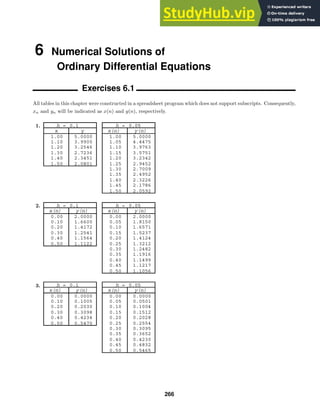
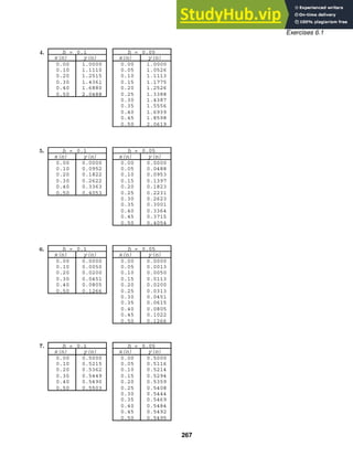
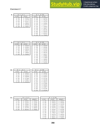


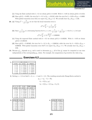
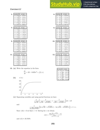
![0 1 2 3 4 5
t
10
20
30
40
50
A(t)
t (days) 1 2 3 4 5
A (observed) 2.78 13.53 36.30 47.50 49.40
A (approximated) 1.93 12.50 36.46 47.23 49.00
A (exact) 1.95 12.64 36.63 47.32 49.02
Exercises 6.2
14. (a) See the table in part (c) of this problem.
(b) From the graph we estimate A(1) ≈ 1.68, A(2) ≈ 13.2, A(3) ≈ 36.8, A(4) ≈ 46.9, and A(5) ≈ 48.9.
(c) Let α = 2.128 and β = 0.0432. Separating variables we obtain
dA
A(α − βA)
= dt
1
α
1
A
+
β
α − βA
dA = dt
1
α
[ln A − ln(α − βA)] = t + c
ln
A
α − βA
= α(t + c)
A
α − βA
= eα(t+c)
A = αeα(t+c)
− βAeα(t+c)
1 + βeα(t+c)
A = αeα(t+c)
.
Thus
A(t) =
αeα(t+c)
1 + βeα(t+c)
=
α
β + e−α(t+c)
=
α
β + e−αce−αt
.
From A(0) = 0.24 we obtain
0.24 =
α
β + e−αc
so that e−αc
= α/0.24 − β ≈ 8.8235 and
A(t) ≈
2.128
0.0432 + 8.8235e−2.128t
.
273](https://image.slidesharecdn.com/advancedengineeringmathematicssolutionsmanual-230807162553-1916df96/85/Advanced-Engineering-Mathematics-Solutions-Manual-pdf-273-320.jpg)
![x
y
2
−5
5
x(n) y(n) x(n) y(n)
0.0 0.0000 1.0 4.2147
0.1 0.1440 1.1 3.8033
0.2 0.5448 1.2 3.1513
0.3 1.1409 1.3 2.3076
0.4 1.8559 1.4 1.3390
0.5 2.6049 1.5 0.3243
0.6 3.3019 1.6 -0.6530
0.7 3.8675 1.7 -1.5117
0.8 4.2356 1.8 -2.1809
0.9 4.3593 1.9 -2.6061
1.0 4.2147 2.0 -2.7539
x
y
2
−5
5
Exercises 6.3
19. (a) Using y(5)
=
24
(x + 1)5
we see that the local truncation error is
y(5)
(c)
h5
120
=
1
(c + 1)5
h5
5
.
(b) Since
1
(x + 1)5
is a decreasing function for 0 ≤ x ≤ 0.5,
1
(c + 1)5
≤
1
(0 + 1)5
= 1 for 0 ≤ c ≤ 0.5 and
y(5)
(c)
h5
5
≤ (1)
(0.1)5
5
= 0.000002.
(c) Using the fourth-order Runge-Kutta method with h = 0.1 we obtain y(0.5) ≈ 0.405465168. With h = 0.05
we obtain y(0.5) ≈ 0.405465111.
20. (a) For y
+ y = 10 sin 3x an integrating factor is ex
so that
d
dx
[ex
y] = 10ex
sin 3x =⇒ ex
y = ex
sin 3x − 3ex
cos 3x + c
=⇒ y = sin 3x − 3 cos 3x + ce−x
.
When x = 0, y = 0, so 0 = −3 + c and c = 3. The solution is y = sin 3x − 3 cos 3x + 3e−x
.
Using Newton’s method we find that x = 1.53235 is the only positive root in [0, 2].
(b) Using the fourth-order Runge-Kutta method with h = 0.1 we obtain the table of values shown. These values
are used to obtain an interpolating function in Mathematica. The graph of the interpolating function is
shown. Using Mathematica’s root finding capability we see that the only positive root in [0, 2] is x = 1.53236.
Exercises 6.3
1. For y
− y = x − 1 an integrating factor is e− dx
= e−x
, so that
d
dx
[e−x
y] = (x − 1)e−x
and
y = ex
(−xe−x
+ c) = −x + cex
.
From y(0) = 1 we find c = 1 and y = −x + ex
. Comparing exact values with approximations obtained in
Example 1, we find y(0.2) ≈ 1.02140276 compared to y1 = 1.02140000, y(0.4) ≈ 1.09182470 compared to
275](https://image.slidesharecdn.com/advancedengineeringmathematicssolutionsmanual-230807162553-1916df96/85/Advanced-Engineering-Mathematics-Solutions-Manual-pdf-275-320.jpg)
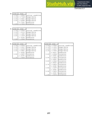
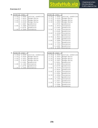
![x(n) y(n) x(n) y(n)
0.00 1.0000 initial condition 0.00 1.0000 initial condition
0.20 1.2337 Runge-Kutta 0.10 1.1079 Runge-Kutta
0.40 1.5531 Runge-Kutta 0.20 1.2337 Runge-Kutta
0.60 1.9961 Runge-Kutta 0.30 1.3807 Runge-Kutta
2.6180 predictor 1.5530 predictor
0.80 2.6214 corrector 0.40 1.5531 corrector
3.5151 predictor 1.7560 predictor
1.00 3.5208 corrector 0.50 1.7561 corrector
1.9960 predictor
0.60 1.9961 corrector
2.2811 predictor
0.70 2.2812 corrector
2.6211 predictor
0.80 2.6213 corrector
3.0289 predictor
0.90 3.0291 corrector
3.5203 predictor
1.00 3.5207 corrector
Exercises 6.4
8.
Exercises 6.4
1. The substitution y
= u leads to the iteration formulas
yn+1 = yn + hun, un+1 = un + h(4un − 4yn).
The initial conditions are y0 = −2 and u0 = 1. Then
y1 = y0 + 0.1u0 = −2 + 0.1(1) = −1.9
u1 = u0 + 0.1(4u0 − 4y0) = 1 + 0.1(4 + 8) = 2.2
y2 = y1 + 0.1u1 = −1.9 + 0.1(2.2) = −1.68.
The general solution of the differential equation is y = c1e2x
+ c2xe2x
. From the initial conditions we find
c1 = −2 and c2 = 5. Thus y = −2e2x
+ 5xe2x
and y(0.2) ≈ 1.4918.
2. The substitution y
= u leads to the iteration formulas
yn+1 = yn + hun, un+1 = un + h
2
x
un −
2
x2
yn
.
The initial conditions are y0 = 4 and u0 = 9. Then
y1 = y0 + 0.1u0 = 4 + 0.1(9) = 4.9
u1 = u0 + 0.1
2
1
u0 −
2
1
y0
= 9 + 0.1[2(9) − 2(4)] = 10
y2 = y1 + 0.1u1 = 4.9 + 0.1(10) = 5.9.
The general solution of the Cauchy-Euler differential equation is y = c1x + c2x2
. From the initial conditions we
find c1 = −1 and c2 = 5. Thus y = −x + 5x2
and y(1.2) = 6.
3. The substitution y
= u leads to the system
y
= u, u
= 4u − 4y.
Using formula (4) in the text with x corresponding to t, y corresponding to x, and u corresponding to y, we
obtain
279](https://image.slidesharecdn.com/advancedengineeringmathematicssolutionsmanual-230807162553-1916df96/85/Advanced-Engineering-Mathematics-Solutions-Manual-pdf-279-320.jpg)
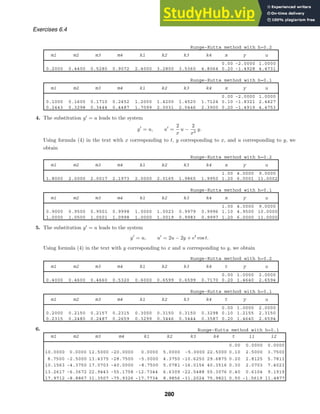
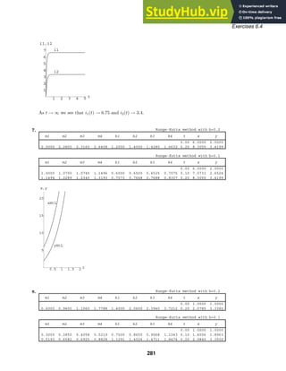
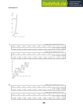
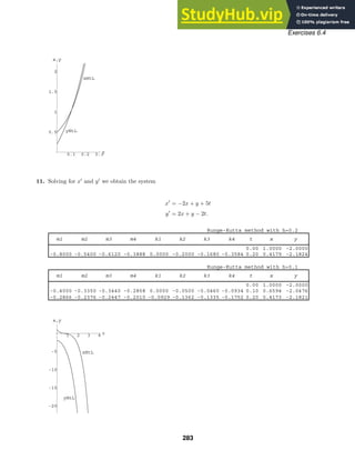
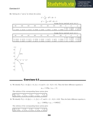
![x 0.0 0.2 0.4 0.6 0.8 1.0
y 0.0000 -0.2259 -0.3356 -0.3308 -0.2167 0.0000
x 0.0 0.2 0.4 0.6 0.8 1.0
y 1.0000 1.9600 3.8800 7.7200 15.4000 0.0000
x 0.0000 0.1667 0.3333 0.5000 0.6667 0.8333 1.0000
y 3.0000 3.3751 3.6306 3.6448 3.2355 2.1411 0.0000
x 1.0000 1.1667 1.3333 1.5000 1.6667 1.8333 2.0000
y 1.0000 -0.5918 -1.1626 -1.3070 -1.2704 -1.1541 -1.0000
x 1.000 1.125 1.250 1.375 1.500 1.625 1.750 1.875 2.000
y 5.0000 3.8842 2.9640 2.2064 1.5826 1.0681 0.6430 0.2913 0.0000
x 1.000 1.125 1.250 1.375 1.500 1.625 1.750 1.875 2.000
y 0.0000 -0.1988 -0.4168 -0.6510 -0.8992 -1.1594 -1.4304 -1.7109 -2.0000
Exercises 6.5
3. We identify P(x) = 2, Q(x) = 1, f(x) = 5x, and h = (1 − 0)/5 = 0.2. Then the finite difference equation is
1.2yi+1 − 1.96yi + 0.8yi−1 = 0.04(5xi).
The solution of the corresponding linear system gives
4. We identify P(x) = −10, Q(x) = 25, f(x) = 1, and h = (1 − 0)/5 = 0.2. Then the finite difference equation is
−yi + 2yi−1 = 0.04.
The solution of the corresponding linear system gives
5. We identify P(x) = −4, Q(x) = 4, f(x) = (1 + x)e2x
, and h = (1 − 0)/6 = 0.1667. Then the finite difference
equation is
0.6667yi+1 − 1.8889yi + 1.3333yi−1 = 0.2778(1 + xi)e2xi
.
The solution of the corresponding linear system gives
6. We identify P(x) = 5, Q(x) = 0, f(x) = 4
√
x , and h = (2 − 1)/6 = 0.1667. Then the finite difference equation
is
1.4167yi+1 − 2yi + 0.5833yi−1 = 0.2778(4
√
xi ).
The solution of the corresponding linear system gives
7. We identify P(x) = 3/x, Q(x) = 3/x2
, f(x) = 0, and h = (2 − 1)/8 = 0.125. Then the finite difference equation
is
1 +
0.1875
xi
yi+1 +
−2 +
0.0469
x2
i
yi +
1 −
0.1875
xi
yi−1 = 0.
The solution of the corresponding linear system gives
8. We identify P(x) = −1/x, Q(x) = x−2
, f(x) = ln x/x2
, and h = (2 − 1)/8 = 0.125. Then the finite difference
equation is
1 −
0.0625
xi
yi+1 +
−2 +
0.0156
x2
i
yi +
1 +
0.0625
xi
yi−1 = 0.0156 ln xi.
The solution of the corresponding linear system gives
9. We identify P(x) = 1 − x, Q(x) = x, f(x) = x, and h = (1 − 0)/10 = 0.1. Then the finite difference equation is
[1 + 0.05(1 − xi)]yi+1 + [−2 + 0.01xi]yi + [1 − 0.05(1 − xi)]yi−1 = 0.01xi.
The solution of the corresponding linear system gives
285](https://image.slidesharecdn.com/advancedengineeringmathematicssolutionsmanual-230807162553-1916df96/85/Advanced-Engineering-Mathematics-Solutions-Manual-pdf-285-320.jpg)
![x 0.0 0.1 0.2 0.3 0.4 0.5 0.6
y 0.0000 0.2660 0.5097 0.7357 0.9471 1.1465 1.3353
0.7 0.8 0.9 1.0
1.5149 1.6855 1.8474 2.0000
x 0.0 0.1 0.2 0.3 0.4 0.5 0.6
y 1.0000 0.8929 0.7789 0.6615 0.5440 0.4296 0.3216
0.7 0.8 0.9 1.0
0.2225 0.1347 0.0601 0.0000
x 0.000 0.125 0.250 0.375 0.500 0.625 0.750 0.875 1.000
y 0.0000 0.3492 0.7202 1.1363 1.6233 2.2118 2.9386 3.8490 5.0000
r 1.0 1.5 2.0 2.5 3.0 3.5 4.0
u 50.0000 72.2222 83.3333 90.0000 94.4444 97.6190 100.0000
Exercises 6.5
10. We identify P(x) = x, Q(x) = 1, f(x) = x, and h = (1 − 0)/10 = 0.1. Then the finite difference equation is
(1 + 0.05xi)yi+1 − 1.99yi + (1 − 0.05xi)yi−1 = 0.01xi.
The solution of the corresponding linear system gives
11. We identify P(x) = 0, Q(x) = −4, f(x) = 0, and h = (1 − 0)/8 = 0.125. Then the finite difference equation is
yi+1 − 2.0625yi + yi−1 = 0.
The solution of the corresponding linear system gives
12. We identify P(r) = 2/r, Q(r) = 0, f(r) = 0, and h = (4 − 1)/6 = 0.5. Then the finite difference equation is
1 +
0.5
ri
ui+1 − 2ui +
1 −
0.5
ri
ui−1 = 0.
The solution of the corresponding linear system gives
13. (a) The difference equation
1 +
h
2
Pi
yi+1 + (−2 + h2
Qi)yi +
1 −
h
2
Pi
yi−1 = h2
fi
is the same as the one derived on page 383 in the text. The equations are the same because the derivation
was based only on the differential equation, not the boundary conditions. If we allow i to range from 0 to
n − 1 we obtain n equations in the n + 1 unknowns y−1, y0, y1, . . . , yn−1. Since yn is one of the given
boundary conditions, it is not an unknown.
(b) Identifying y0 = y(0), y−1 = y(0 − h), and y1 = y(0 + h) we have from (5) in the text
1
2h
[y1 − y−1] = y
(0) = 1 or y1 − y−1 = 2h.
The difference equation corresponding to i = 0,
1 +
h
2
P0
y1 + (−2 + h2
Q0)y0 +
1 −
h
2
P0
y−1 = h2
f0
becomes, with y−1 = y1 − 2h,
1 +
h
2
P0
y1 + (−2 + h2
Q0)y0 +
1 −
h
2
P0
(y1 − 2h) = h2
f0
or
2y1 + (−2 + h2
Q0)y0 = h2
f0 + 2h − P0.
286](https://image.slidesharecdn.com/advancedengineeringmathematicssolutionsmanual-230807162553-1916df96/85/Advanced-Engineering-Mathematics-Solutions-Manual-pdf-286-320.jpg)
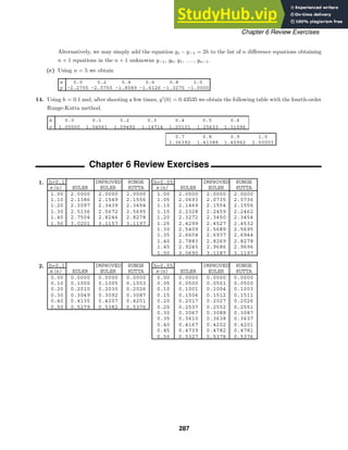
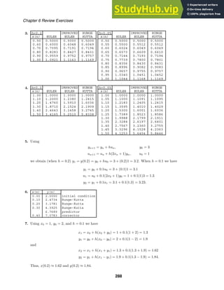
![x 0.0 0.1 0.2 0.3 0.4 0.5 0.6
y 0.0000 4.1987 8.1049 11.3840 13.7038 14.7770 14.4083
0.7 0.8 0.9 1.0
12.5396 9.2847 4.9450 0.0000
Chapter 6 Review Exercises
8. We identify P(x) = 0, Q(x) = 6.55(1 + x), f(x) = 1, and h = (1 − 0)/10 = 0.1. Then the finite difference
equation is
yi+1 + [−2 + 0.0655(1 + xi)]yi + yi−1 = 0.001
or
yi+1 + (0.0655xi − 1.9345)yi + yi−1 = 0.001.
The solution of the corresponding linear system gives
289](https://image.slidesharecdn.com/advancedengineeringmathematicssolutionsmanual-230807162553-1916df96/85/Advanced-Engineering-Mathematics-Solutions-Manual-pdf-289-320.jpg)
![Exercises 7.1
(b) θ = tan−1
0.6 ≈ 31◦
.
46. Since w + F1 + F2 = 0,
−200j + F1 cos 20◦
i + F1 sin 20◦
j − F2 cos 15◦
i + F2 sin 15◦
j = 0
or (F1 cos 20◦
− F2 cos 15◦
)i + (F1 sin 20◦
+ F2 sin 15◦
− 200)j = 0.
Thus, F1 cos 20◦
− F2 cos 15◦
= 0; F1 sin 20◦
+ F2 sin 15◦
− 200 = 0. Solving this system for F1 and
F2, we obtain
F1 =
200 cos 15◦
sin 15◦ cos 20◦ + cos 15◦ sin 20◦
=
200 cos 15◦
sin(15◦ + 20◦)
=
200 cos 15◦
sin 35◦
≈ 336.8 lb
and
F2 =
200 cos 20◦
sin 15◦ cos 20◦ + cos 15◦ sin 20◦
=
200 cos 20◦
sin 35◦
≈ 327.7 lb.
47. Since y/2a(L2
+ y2
)3/2
is an odd function on [−a, a], Fy = 0. Now, using the fact that L/(L2
+ y2
)3/2
is an
even function, we have
a
−a
L dy
2a(L2 + y2)3/2
=
L
a
a
0
dy
(L2 + y2)3/2
y = L tan θ, dy = L sec2
θ dθ
=
L
a
tan−1
a/L
0
L sec2
θ dθ
L3(1 + tan2
θ)3/2
=
1
La
tan−1
a/L
0
sec2
θ dθ
sec3 θ
=
1
La
tan−1
a/L
0
cos θ dθ =
1
La
sin θ
tan−1
a/L
0
=
1
La
a
√
L2 + a2
=
1
L
√
L2 + a2
.
Then Fx = qQ/4π0L
√
L2 + a2 and F = (qQ/4π0L
√
L2 + a2 )i.
48. Place one corner of the parallelogram at the origin and let two adja-
cent sides be
−
−
→
OP1 and
−
−
→
OP2. Let M be the midpoint of the diagonal
connecting P1 and P2 and N be the midpoint of the other diagonal.
By Problem 37,
−
−
→
OM = 1
2 (
−
−
→
OP1 +
−
−
→
OP2). Since
−
−
→
OP1 +
−
−
→
OP2 is the main diagonal of the parallelogram and N is
its midpoint,
−
−
→
ON = 1
2 (
−
−
→
OP1 +
−
−
→
OP2). Thus,
−
−
→
OM =
−
−
→
ON and the diagonals bisect each other.
49. By Problem 39,
−
−
→
AB +
−
−
→
BC +
−
→
CA = 0 and
−
−
→
AD +
−
−
→
DE +
−
−
→
EC +
−
→
CA = 0. From the first equation,
−
−
→
AB +
−
−
→
BC = −
−
→
CA. Since D and E are midpoints,
−
−
→
AD = 1
2
−
−
→
AB and
−
−
→
EC = 1
2
−
−
→
BC. Then,
1
2
−
−
→
AB +
−
−
→
DE + 1
2
−
−
→
BC +
−
→
CA = 0 and
−
−
→
DE = −
−
→
CA −
1
2
(
−
−
→
AB +
−
−
→
BC) = −
−
→
CA −
1
2
(−
−
→
CA) = −
1
2
−
→
CA.
Thus, the line segment joining the midpoints D and E is parallel to the side AC and half its length.
50. We have
−
→
OA = 150 cos 20◦
i+150 sin 20◦
j,
−
−
→
AB = 200 cos 113◦
i+200 sin 113◦
j,
−
−
→
BC = 240 cos 190◦
i+240 sin 190◦
j.
Then
r = (150 cos 20◦
+ 200 cos 113◦
+ 240 cos 190◦
)i + (150 sin 20◦
+ 200 sin 113◦
+ 240 sin 190◦
)j
≈ −173.55i + 193.73j
and r ≈ 260.09 miles.
292](https://image.slidesharecdn.com/advancedengineeringmathematicssolutionsmanual-230807162553-1916df96/85/Advanced-Engineering-Mathematics-Solutions-Manual-pdf-292-320.jpg)

![Exercises 7.3
43. b + 2(a − 3c) = −1, 1, 1 + 2−5, −21, −25 = −11, −41, −49
44. 4(a + 2c) − 6b = 45, 9, 20 − −6, 6, 6 = 26, 30, 74
45. a + c = 3, 3, 11 =
√
9 + 9 + 121 =
√
139
46. c2b = (
√
4 + 36 + 81 )(2)(
√
1 + 1 + 1 ) = 22
√
3
47.
a
a
+ 5
b
|b
=
1
a
a + 5
1
b
b = 1 + 5 = 6
48. ba + ab =
√
1 + 1 + 1 1, −3, 2 +
√
1 + 9 + 4 −1, 1, 1 =
√
3 , −3
√
3 , 2
√
3 + −
√
14 ,
√
14 ,
√
14
=
√
3 −
√
14 , −3
√
3 +
√
14 , 2
√
3 +
√
14
49. a =
√
100 + 25 + 100 = 15; u = −
1
15
10, −5, 10 = −2/3, 1/3, −2/3
50. a =
√
1 + 9 + 4 =
√
14 ; u =
1
√
14
(i − 3j + 2k) =
1
√
14
i −
3
√
14
j +
2
√
14
k
51. b = 4a = 4i − 4j + 4k
52. a =
√
36 + 9 + 4 = 7; b = −
1
2
1
7
−6, 3, −2 =
3
7
, −
3
14
,
1
7
53.
Exercises 7.3
1. a · b = 10(5) cos(π/4) = 25
√
2 2. a · b = 6(12) cos(π/6) = 36
√
3
3. a · b = 2(−1) + (−3)2 + 4(5) = 12 4. b · c = (−1)3 + 2(6) + 5(−1) = 4
5. a · c = 2(3) + (−3)6 + 4(−1) = −16 6. a · (b + c) = 2(2) + (−3)8 + 4(4) = −4
7. a · (4b) = 2(−4) + (−3)8 + 4(20) = 48 8. b · (a − c) = (−1)(−1) + 2(−9) + 5(5) = 8
9. a · a = 22
+ (−3)2
+ 42
= 29 10. (2b) · (3c) = (−2)9 + 4(18) + 10(−3) = 24
11. a · (a + b + c) = 2(4) + (−3)5 + 4(8) = 25
12. (2a) · (a − 2b) = 4(4) + (−6)(−7) + 8(−6) = 10
13.
a · b
b · b
b =
2(−1) + (−3)2 + 4(5)
(−1)2 + 22 + 52
−1, 2, 5 =
12
30
−1, 2, 5 = −2/5, 4/5, 2
14. (c · b)a = [3(−1) + 6(2) + (−1)5]2, −3, 4 = 42, −3, 4 = 8, −12, 16
15. a and f, b and e, c and d
16. (a) a · b = 2 · 3 + (−c)2 + 3(4) = 0 =⇒ c = 9
295](https://image.slidesharecdn.com/advancedengineeringmathematicssolutionsmanual-230807162553-1916df96/85/Advanced-Engineering-Mathematics-Solutions-Manual-pdf-295-320.jpg)
![Exercises 7.4
17. (a) b × c =
i j k
2 1 1
3 1 1
=
1 1
1 1
i −
2 1
3 1
j +
2 1
3 1
k = j − k
a × (b × c) =
i j k
1 −1 2
0 1 −1
=
−1 2
1 −1
i −
1 2
0 −1
j +
1 −1
0 1
k = −i + j + k
(b) a · c = (i − j + 2k) · (3i + j + k) = 4; (a · c)b = 4(2i + j + k) = 8i + 4j + 4k
a · b = (i − j + 2k) · (2i + j + k) = 3; (a · b)c = 3(3i + j + k) = 9i + 3j + 3k
a × (b × c) = (a · c)b − (a · b)c = (8i + 4j + 4k) − (9i + 3j + 3k) = −i + j + k
18. (a) b × c =
i j k
1 2 −1
−1 5 8
=
2 −1
5 8
i −
1 −1
−1 8
j +
1 2
−1 5
k = 21i − 7j + 7k
a × (b × c) =
i j k
3 0 −4
21 −7 7
=
0 −4
−7 7
i −
3 −4
21 7
j +
3 0
21 −7
k = −28i − 105j − 21k
(b) a · c = (3i − 4k) · (−i + 5j + 8k) = −35; (a · c)b = −35(i + 2j − k) = −35i − 70j + 35k
a · b = (3i − 4k) · (i + 2j − k) = 7; (a · b)c = 7(−i + 5j + 8k) = −7i + 35j + 56k
a × (b × c) = (a · c)b − (a · b)c = (−35i − 70j + 35k) − (−7i + 35j + 56k) = −28i − 105j − 21k
19. (2i) × j = 2(i × j) = 2k
20. i × (−3k) = −3(i × k) = −3(−j) = 3j
21. k × (2i − j) = k × (2i) + k × (−j) = 2(k × i) − (k × j) = 2j − (−i) = i + 2j
22. i × (j × k) = i × i = 0
23. [(2k) × (3j)] × (4j) = [2 · 3(k × j) × (4j)] = 6(−i) × 4j = (−6)(4)(i × j) = −24k
24. (2i − j + 5k) × i = (2i × i) + (−j × i) + (5k × i) = 2(i × i) + (i × j) + 5(k × i) = 5j + k
25. (i + j) × (i + 5k) = [(i + j) × i] + [(i + j) × 5k] = (i × i) + (j × i) + (i × 5k) + (j × 5k)
= −k + 5(−j) + 5i = 5i − 5j − k
26. i × k − 2(j × i) = −j − 2(−k) = −j + 2k
27. k · (j × k) = k · i = 0
28. i · [j × (−k)] = i · [−(j × k)] = i · (−i) = −(i · i) = −1
29. 4j − 5(i × j) = 4j − 5k =
√
41
30. (i × j) · (3j × i) = k · (−3k) = −3(k · k) = −3
31. i × (i × j) = i × k = −j 32. (i × j) × i = k × i = j
33. (i × i) × j = 0 × j = 0 34. (i · i)(i × j) = 1(k) = k
35. 2j · [i × (j − 3k)] = 2j · [(i × j) + (i × (−3k)] = 2j · [k + 3(k × i)] = 2j · (k + 3j) = 2j · k + 2j · 3j
= 2(j · k) + 6(j · j) = 2(0) + 6(1) = 6
36. (i × k) × (j × i) = (−j) × (−k) = (−1)(−1)(j × k) = j × k = i
37. a × (3b) = 3(a × b) = 3(4i − 3j + 6k) = 12i − 9j + 18k
38. b × a = −a × b = −(a × b) = −4i + 3j − 6k
39. (−a) × b = −(a × b) = −4i + 3j − 6k
300](https://image.slidesharecdn.com/advancedengineeringmathematicssolutionsmanual-230807162553-1916df96/85/Advanced-Engineering-Mathematics-Solutions-Manual-pdf-300-320.jpg)

![Exercises 7.4
51. b × c =
i j k
−1 4 0
2 2 2
=
4 0
2 2
i −
−1 0
2 2
j +
−1 4
2 2
k = 8i + 2j − 10k
v = |a · (b × c)| = |(i + j) · (8i + 2j − 10k)| = |8 + 2 + 0| = 10 cu. units
52. b × c =
i j k
1 4 1
1 1 5
=
4 1
1 5
i −
1 1
1 5
j +
1 4
1 1
k = 19i − 4j − 3k
v = |a · (b × c)| = |(3i + j + k) · (19i − 4j − 3k)| = |57 − 4 − 3| = 50 cu. units
53. b × c =
i j k
−2 6 −6
5/2 3 1/2
=
6 −6
3 2/2
i −
−2 −6
5/2 1/2
j +
−2 6
5/2 3
k = 21i − 14j − 21k
a · (b × c) = (4i + 6j) · (21i − 14j − 21k) = 84 − 84 + 0 = 0. The vectors are coplanar.
54. The four points will be coplanar if the three vectors
−
−
−
→
P1P2 = 3, −1, −1,
−
−
−
→
P2P3 = −3, −5, 13, and
−
−
−
→
P3P4 =
−8, 7, −6 are coplanar.
−
−
−
→
P2P3 ×
−
−
−
→
P3P4 =
i j k
−3 −5 13
−8 7 −6
=
−5 13
7 −6
i −
−3 13
−8 −6
j +
−3 −5
−8 7
k = −61, −122, −61
−
−
−
→
P1P2 · (
−
−
−
→
P2P3 ×
−
−
−
→
P3P4) = 3, −1, −1 · −61, −122, −61 = −183 + 122 + 61 = 0
The four points are coplanar.
55. (a) Since θ = 90◦
, a × b = a b | sin 90◦
| = 6.4(5) = 32.
(b) The direction of a × b is into the fourth quadrant of the xy-plane or to the left of the plane determined by
a and b as shown in Figure 6.54 in the text. It makes an angle of 30◦
with the positive x-axis.
(c) We identify n = (
√
3 i − j)/2. Then a × b = 32n = 16
√
3 i − 16j.
56. Using Definition 7.4, a × b =
√
27 (8) sin 120◦
n = 24
√
3 (
√
3/2)n = 36n. By the right-hand rule, n = j or
n = −j. Thus, a × b = 36j or −36j.
57. (a) We note first that a × b = k, b × c = 1
2 (i − k), c × a = 1
2 (j − k), a · (b × c) = 1
2 , b · (c × a) = 1
2 , and
c · (a × b) = 1
2 . Then
A =
1
2 (i − k)
1
2
= i − k, B =
1
2 (j − k)
1
2
= j − k, and C =
k
1
2
= 2k.
(b) We need to compute A · (B × C). Using formula (10) in the text we have
B × C =
(c × a) × (a × b)
[b · (c × a)][c · (a × b)]
=
[(c × a) · b]a − [(c × a) · a]b
[b · (c × a)][c · (a × b)]
=
a
c · (a × b)
since (c × a) · a = 0.
Then
A · (B × C) =
b × c
a · (b × c)
·
a
c · (a × b)
=
1
c · (a × b)
and the volume of the unit cell of the reciprocal latrice is the reciprocal of the volume of the unit cell of
the original lattice.
302](https://image.slidesharecdn.com/advancedengineeringmathematicssolutionsmanual-230807162553-1916df96/85/Advanced-Engineering-Mathematics-Solutions-Manual-pdf-302-320.jpg)
![Exercises 7.4
58. a × (b + c) =
a2 a3
b2 + c2 b3 + c3
i −
a1 a3
b1 + c1 b3 + c3
j +
a1 a2
b1 + c1 b2 + c2
k
= (a2b3 − a3b2)i + (a2c3 − a3c2)i − [(a1b3 − a3b1)j + (a1c3 − a3c1)j] + (a1b2 − a2b1)k + (a1c2 − a2c1)k
= (a2b3 − a3b2)i − (a1b3 − a3b1)j + (a1b2 − a2b1)k + (a2c3 − a3c2)i − (a1c3 − a3c1)j + (a1c2 − a2c1)k
= a × b + a × c
59. b × c = (b2c3 − b3c2)i − (b1c3 − b3c1)j + (b1c2 − b2c1)k
a × (b × c) = [a2(b1c2 − b2c1) + a3(b1c3 − b3c1)]i − [a1(b1c2 − b2c1) − a3(b2c3 − b3c2)]j
+ [−a1(b1c3 − b3c1) − a2(b2c3 − b3c2)]k
= (a2b1c2 − a2b2c1 + a3b1c3 − a3b3c1)i − (a1b1c2 − a1b2c1 − a3b2c3 + a3b3c2)j
− (a1b1c3 − a1b3c1 + a2b2c3 − a2b3c2)k
(a · c)b − (a · b)c = (a1c1 + a2c2 + a3c3)(b1i + b2j + b3k) − (a1b1 + a2b2 + a3b3)(c1i + c2j + c3k)
= (a2b1c2 − a2b2c1 + a3b1c3 − a3b3c1)i − (a1b1c2 − a1b2c1 − a3b2c3 + a3b3c2)j
− (a1b1c3 − a1b3c1 + a2b2c3 − a2b3c2)k
60. The statement is false since i × (i × j) = i × k = −j and (i × i) × j = 0 × j = 0.
61. Using equation 9 in the text,
a · (b × c) =
a1 a2 a3
b1 b2 b3
c1 c2 c3
and (a × b) · c = c · (a × b) =
c1 c2 c3
a1 a2 a3
b1 b2 b3
.
The second determinant can be obtained from the first by an interchange of the second and third rows followed by
an interchange of the new first and second rows. Using Theorem 8.11 in the text, we see that a·(b×c) = (a×b)·c.
62. a × (b × c) + b × (c × a) + c × (a × b)
= (a · c)b − (a · b)c + (b · a)c − (b · c)a + (c · b)a − (c · a)b
= [(a · c)b − (c · a)b] + [(b · a)c − (a · b)c] + [(c · b)a − (b · c)a] = 0
63. Since
a × b2
= (a2b3 − a3b2)2
+ (a1b3 − a3b1)2
+ (a1b2 − a2b1)2
= a2
2b2
3 − 2a2b3a3b2 + a2
3b2
2 + a2
1b2
3 − 2a1b3a3b1 + a2
3b2
1 + a2
1b2
2 − 2a1b2a2b1 + a2
2b2
1
and
a2
b2
− (a · b)2
= (a2
1 + a2
2 + a2
3)(b2
1 + b2
2 + b2
3) − (a1b1 + a2b2 + a3b3)2
= a2
1a2
2 + a2
1b2
2 + a2
1b2
3 + a2
2b2
1 + a2
2b2
2 + a2
2b2
3 + a2
3b2
1 + a2
3b2
2 + a2
3b2
3
− a2
1b2
1 − a2
2b2
2 − a2
3b2
3 − 2a1b1a2b2 − 2a1b1a3b3 − 2a2b2a3b3
= a2
1b2
2 + a2
1b2
3 + a2
2b2
1 + a2
2b2
3 + a2
3b2
1 + a2
3b2
2 − 2a1a2b1b2 − 2a1a3b1b3 − 2a2a3b2b3
we see that a × b2
= a2
b2
− (a · b)2
.
64. No. For example i × (i + j) = i × j by the distributive law (iii) in the text, and the fact that i × i = 0. But i + j
does not equal j.
65. By the distributive law (iii) in the text:
(a + b) × (a − b) = (a + b) × a − (a + b) × b = a × a + b × a − a × b − b × b = 2b × a
since a × a = 0, b × b = 0, and −a × b = b × a.
303](https://image.slidesharecdn.com/advancedengineeringmathematicssolutionsmanual-230807162553-1916df96/85/Advanced-Engineering-Mathematics-Solutions-Manual-pdf-303-320.jpg)


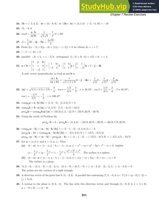
![Chapter 7 Review Exercises
41. The direction vectors are −2, 3, 1 and 2, 1, 1. Since −2, 3, 1 · 2, 1, 1 = 0, the lines are orthogonal. Solving
1 − 2t = x = 1 + 2s, 3t = y = −4 + s, we obtain t = −1 and s = 1. The point (3, −3, 0) obtained by letting
t = −1 and s = 1 is common to the two lines, so they do intersect.
42. Vectors in the plane are 2, 3, 1 and 1, 0, 2. A normal vector is 2, 3, 1×1, 0, 2 = 6, −3, −3 = 32, −1, −1.
An equation of the plane is 2x − y − z = 0
43. The lines are parallel with direction vector 1, 4, −2. Since (0, 0, 0) is on the first line and (1, 1, 3) is on the second
line, the vector 1, 1, 3 is in the plane. A normal vector to the plane is thus 1, 4, −2 × 1, 1, 3 = 14, −5, −3.
An equation of the plane is 14x − 5y − 3z = 0.
44. Letting z = t in the equations of the plane and solving −x + y = 4 + 8t, 3x − y = −2t, we obtain x = 2 + 3t,
y = 6 + 11t, z = t. Thus, a normal to the plane is 3, 11, 1 and an equation of the plane is
3(x − 1) + 11(y − 7) + (z + 1) = 0 or 3x + 11y + z = 79.
45. F = 10
a
a
=
10
√
2
(i + j) = 5
√
2 i + 5
√
2 j; d = 7, 4, 0 − 4, 1, 0 = 3i + 3j
W = F · d = 15
√
2 + 15
√
2 = 30
√
2 N-m
46. F = 5
√
2 i + 5
√
2 j + 50i = (5
√
2 + 50)i + 5
√
2 j; d = 3i + 3j
W = 15
√
2 + 150 + 15
√
2 = 30
√
2 + 150 N-m ≈ 192.4 N-m
47. Since F2 = 200(i + j)/
√
2 = 100
√
2 i + 100
√
2 j, F3 = F2 − F1 = (100
√
2 − 200)i + 100
√
2 j and
F3 =
(100
√
2 − 200)2 + (100
√
2)2 = 200
2 −
√
2 ≈ 153 lb.
48. Let F1 = F1 and F2 = F2. Then F1 = F1[(cos 45◦
)i + (sin 45◦
)j] and F2 = F2[(cos 120◦
)i + (sin 120◦
)j], or
F1 = F1( 1
√
2
i + 1
√
2
j) and F2 = F2(−1
2 i +
√
3
2 j). Since w + F1 + F2 = 0,
F1(
1
√
2
i +
1
√
2
j) + F2(−
1
2
i +
√
3
2
j) = 50j, (
1
√
2
F1 −
1
2
F2)i + (
1
√
2
F1 +
√
3
2
F2)j = 50j
and
1
√
2
F1 −
1
2
F2 = 0,
1
√
2
F1 +
√
3
2
F2 = 50.
Solving, we obtain F1 = 25(
√
6 −
√
2 ) ≈ 25.9 lb and F2 = 50(
√
3 − 1) ≈ 36.6 lb.
49. Not a vector space. Axiom (viii) is not satisfied.
50. The vectors are linearly independent. The only solution of the system
c1 = 0, c1 + 2c2 + c3 = 0, 2c1 + 3c2 − c3 = 0
is c1 = 0, c2 = 0, c3 = 0.
51. Let p1 and p2 be in Pn such that
d2
p1
dx2
= 0 and
d2
p2
dx2
= 0. Since
0 =
d2
p1
dx2
+
d2
p2
dx2
=
d2
dx2
(p1 + p2) and 0 = k
d2
p1
dx2
=
d2
dx2
(kp1)
we conclude that the set of polynomials with the given property is a subspace of Pn. A basis for the subspace
is 1, x.
52. The intersection W1 ∩ W2 is a subspace of V . If x and y are in W1 ∩ W2 then x and y are in each subspace
and so x + y is in each subspace. That is, x + y is in W1 ∩ W2. Similarly, if x is in W1 ∩ W2 then x is in each
subspace and so kx is in each subspace. That is, kx is in W1 ∩ W2 for any scalar k.
The union W1 ∪W2 is generally not a subspace. For example, W1 = {x, y
y = x} and W2 = {x, y
y = 2x}
are subspaces of R2
. Now 1, 1 is in W1 and 1, 2 is in W2 but 1, 1 + 1, 2 = 2, 3 is not in W1 ∪ W2.
312](https://image.slidesharecdn.com/advancedengineeringmathematicssolutionsmanual-230807162553-1916df96/85/Advanced-Engineering-Mathematics-Solutions-Manual-pdf-312-320.jpg)
![Exercises 8.1
(b) BA =
−4 + 30 − 24 −16 + 60 − 36
1 − 15 + 16 4 − 30 + 24
=
2 8
2 −2
19. (a) BC =
9 24
3 8
(b) A(BC) =
1 −2
−2 4
9 24
3 8
=
3 8
−6 −16
(c) C(BA) =
0 2
3 4
0 0
0 0
=
0 0
0 0
(d) A(B + C) =
1 −2
−2 4
6 5
5 5
=
−4 −5
8 10
20. (a) AB = [ 5 −6 7 ]
3
4
−1
= (−16)
(b) BA =
3
4
−1
[ 5 −6 7 ] =
15 −18 21
20 −24 28
−5 6 −7
(c) (BA)C =
15 −18 21
20 −24 28
−5 6 −7
1 2 4
0 1 −1
3 2 1
=
78 54 99
104 72 132
−26 −18 −33
(d) Since AB is 1 × 1 and C is 3 × 3 the product (AB)C is not defined.
21. (a) AT
A = [ 4 8 −10 ]
4
8
−10
= (180)
(b) BT
B =
2
4
5
[ 2 4 5 ] =
4 8 10
8 16 20
10 20 25
(c) A + BT
=
4
8
−10
+
2
4
5
=
6
12
−5
22. (a) A + BT
=
1 2
2 4
+
−2 5
3 7
=
−1 7
5 11
(b) 2AT
− BT
=
2 4
4 8
−
−2 5
3 7
=
4 −1
1 1
(c) AT
(A − B) =
1 2
2 4
3 −1
−3 −3
=
−3 −7
−6 −14
23. (a) (AB)T
=
7 10
38 75
T
=
7 38
10 75
314](https://image.slidesharecdn.com/advancedengineeringmathematicssolutionsmanual-230807162553-1916df96/85/Advanced-Engineering-Mathematics-Solutions-Manual-pdf-314-320.jpg)
![Exercises 8.1
(b) BT
AT
=
5 −2
10 −5
3 8
4 1
=
7 38
10 75
24. (a) AT
+ B =
5 −4
9 6
+
−3 11
−7 2
=
2 7
2 8
(b) 2A + BT
=
10 18
−8 12
+
−3 −7
11 2
=
7 11
3 14
25.
−4
8
−
4
16
+
−6
9
=
−14
1
26.
6
3
−3
+
−5
−5
15
+
−6
−8
10
=
−5
−10
22
27.
−19
18
−
19
20
=
−38
−2
28.
−7
17
−6
+
−1
1
4
−
2
8
−6
=
−10
10
4
29. 4 × 5 30. 3 × 2
31. AT
=
2 −3
4 2
; (AT
)T
=
2 4
−3 2
= A 32. (A + B)T
=
6 −6
14 10
= AT
+ BT
33. (AB)T
=
16 40
−8 −20
T
=
16 −8
40 −20
; BT
AT
=
4 2
10 5
2 −3
4 2
=
16 −8
40 −20
34. (6A)T
=
12 −18
24 12
= 6AT
35. B = AAT
=
2 1
6 3
2 5
2 6 2
1 3 5
=
5 15 9
15 39 27
9 27 29
= BT
36. Using Problem 33 we have (AAT
)T
= (AT
)T
AT
= AAT
, so that AAT
is symmetric.
37. Let A =
1 0
0 0
and B =
0 0
0 1
. Then AB = 0.
38. We see that A = B, but AC =
2 3 4
4 6 8
6 9 12
= BC.
39. Since (A+B)2
= (A+B)(A+B) = A2
+AB+BA+B2
, and AB = BA in general, (A+B)2
= A2
+2AB+B2
.
40. Since (A + B)(A − B) = A2
− AB + BA − B2
, and AB = BA in general, (A + B)(A − B) = A2
− B2
.
41. a11x1 + a12x2 = b1; a21x1 + a22x2 = b2
42.
2 6 1
1 2 −1
5 7 −4
x1
x2
x3
=
7
−1
9
43. [ x y ]
a b/2
b/2 c
x
y
= [ ax + by/2 bx/2 + cy ]
x
y
= [ ax2
+ bxy/2 + bxy/2 + cy2
] = [ ax2
+ bxy + cy2
]
44.
0 −∂/∂z ∂/∂y
∂/∂z 0 −∂/∂x
−∂/∂y ∂/∂x 0
P
Q
R
=
−∂Q/∂z + ∂R/∂y
∂P/∂z − ∂R/∂x
−∂P/∂y + ∂Q/∂x
= curl F
315](https://image.slidesharecdn.com/advancedengineeringmathematicssolutionsmanual-230807162553-1916df96/85/Advanced-Engineering-Mathematics-Solutions-Manual-pdf-315-320.jpg)
![Exercises 8.1
45. (a) MY
x
y
z
=
cos γ sin γ 0
− sin γ cos γ 0
0 0 1
x
y
z
=
x cos γ + y sin γ
−x sin γ + y cos γ
z
=
xY
yY
zY
(b) MR =
cos β 0 − sin β
0 1 0
sin β 0 cos β
; MP
1 0 0
0 cos α sin α
0 − sin α cos α
(c) MP
1
1
1
=
1 0 0
0 cos 30◦
sin 30◦
0 − sin 30◦
cos 30◦
1
1
1
=
1 0 0
0
√
3
2
1
2
0 −1
2
√
3
2
1
1
1
=
1
1
2 (
√
3 + 1)
1
2 (
√
3 − 1)
MRMP
1
1
1
=
cos 45◦
0 − sin 45◦
0 1 0
sin 45◦
0 cos 45◦
1
1
2 (
√
3 + 1)
1
2 (
√
3 − 1)
=
√
2
2 0 −
√
2
2
0 1 0
√
2
2 0
√
2
2
1
1
2 (
√
3 + 1)
1
2 (
√
3 − 1)
=
1
4 (3
√
2 −
√
6 )
1
2 (
√
3 + 1)
1
4 (
√
2 +
√
6 )
MY MRMP
1
1
1
=
cos 60◦
sin 60◦
0
− sin 60◦
cos 60◦
0
0 0 1
1
4 (3
√
2 −
√
6 )
1
2 (
√
3 + 1)
1
4 (
√
2 +
√
6 )
=
1
2
√
3
2 0
−
√
3
2
1
2 0
0 0 1
1
4 (3
√
2 −
√
6 )
1
2 (
√
3 + 1)
1
4 (
√
2 +
√
6 )
=
1
8 (3
√
2 −
√
6 + 6 + 2
√
3 )
1
8 (−3
√
6 + 3
√
2 + 2
√
3 + 2)
1
4 (
√
2 +
√
6 )
46. (a) LU =
1 0
1
2 1
2 −2
0 3
=
2 −2
1 2
= A
(b) LU =
1 0
2
3 1
6 2
0 −1
3
=
6 2
4 1
= A
(c) LU =
1 0 0
0 1 0
2 10 1
1 −2 1
0 1 2
0 0 −21
=
1 −2 1
0 1 2
2 6 1
= A
(d) LU =
1 0 0
3 1 0
1 1 1
1 1 1
0 −2 −1
0 0 1
=
1 1 1
3 1 2
1 −1 1
= A
47. (a) AB =
A11 A12
A21 A22
B1
B2
=
A11B1 + A12B2
A21B1 + A22B2
=
17 43
3 75
−14 51
since
A11B1 + A12B2 =
13 25
−9 49
+
4 18
12 26
=
17 43
3 75
and
A21B1 + A22B2 = [ −24 34 ] + [ 10 17 ] = [ −14 51 ] .
316](https://image.slidesharecdn.com/advancedengineeringmathematicssolutionsmanual-230807162553-1916df96/85/Advanced-Engineering-Mathematics-Solutions-Manual-pdf-316-320.jpg)

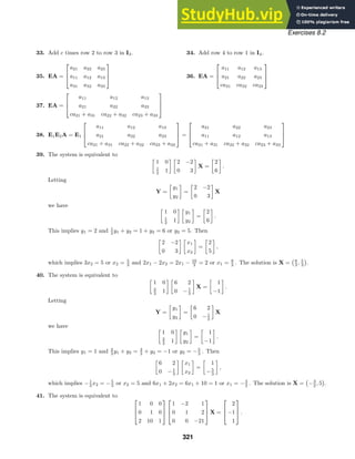
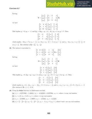


![Exercises 8.8
be stochastic matrices. Then
AB =
a11b11 + a12b21 a11b12 + a12b22
a21b11 + a22b21 a21b12 + a22b22
.
The sums of the rows are
a11b11 + a12b21 + a11b12 + a12b22 = a11(b11 + b12) + a12(b21 + b22)
= a11(1) + a12(1) = a11 + a12 = 1
a21b11 + a22b21 + a21b12 + a22b22 = a21(b11 + b12) + a22(b21 + b22)
= a21(1) + a22(1) = a21 + a22 = 1.
Thus, the product matrix AB is stochastic. It follows that any power of a 2 × 2 matrix is stochastic. The
proof in the case of an n × n matrix is very similar.
Exercises 8.9
1. The characteristic equation is λ2
− 6λ + 13 = 0. Then
A2
− 6A + 13I =
−7 −12
24 17
−
6 −12
24 30
+
13 0
0 13
=
0 0
0 0
.
2. The characteristic equation is −λ3
+ λ2
+ 4λ − 1. Then
−A3
+ A2
+ A − I = −
2 6 13
4 5 17
1 5 9
+
1 2 5
0 4 5
1 1 4
+ 4
0 1 2
1 0 3
0 1 1
+
1 0 0
0 1 0
0 0 1
=
0 0 0
0 0 0
0 0 0
.
3. The characteristic equation is λ2
− 3λ − 10 = 0, with eigenvalues −2 and 5. Substituting the eigenvalues into
λm
= c0 + c1λ generates
(−2)m
= c0 − 2c1
5m
= c0 + 5c1.
Solving the system gives
c0 =
1
7
[5(−2)m
+ 2(5)m
], c1 =
1
7
[−(−2)m
+ 5m
].
Thus
Am
= c0I + c1A =
1
7 [3(−1)m
2m+1
+ 5m
] 3
7 [−(−2)m
+ 5m
]
2
7 [−(−2)m
+ 5m
] 1
7 [(−2)m
+ 6(5)m
]
and
A3
=
11 57
38 106
.
4. The characteristic equation is λ2
− 10λ + 16 = 0, with eigenvalues 2 and 8. Substituting the eigenvalues into
λm
= c0 + c1λ generates
2m
= c0 + 2c1
8m
= c0 + 8c1.
Solving the system gives
c0 =
1
3
(2m+2
− 8m
), c1 =
1
6
(−2m
+ 8m
).
342](https://image.slidesharecdn.com/advancedengineeringmathematicssolutionsmanual-230807162553-1916df96/85/Advanced-Engineering-Mathematics-Solutions-Manual-pdf-342-320.jpg)
![Exercises 8.9
Thus
Am
= c0I + c1A =
1
2 (2m
+ 8m
) 1
2 (2m
− 8m
)
1
2 (2m
− 8m
) 1
2 (2m
+ 8m
)
and
A4
=
2056 −2040
−2040 2056
.
5. The characteristic equation is λ2
− 8λ − 20 = 0, with eigenvalues −2 and 10. Substituting the eigenvalues into
λm
= c0 + c1λ generates
(−2)m
= c0 − 2c1
10m
= c0 + 10c1.
Solving the system gives
c0 =
1
6
[5(−2)m
+ 10m
], c1 =
1
12
[−(−2)m
+ 10m
].
Thus
Am
= c0I + c1A =
1
6 [(−2)m
+ 2m
5m+1
] 5
12 [−(−2)m
+ 10m
]
1
3 [−(−2)m
+ 10m
] 1
6 [5(−2)m
+ 10m
]
and
A5
=
83328 41680
33344 16640
.
6. The characteristic equation is λ2
+ 4λ + 3 = 0, with eigenvalues −3 and −1. Substituting the eigenvalues into
λm
= c0 + c1λ generates
(−3)m
= c0 − 3c1
(−1)m
= c0 − c1.
Solving the system gives
c0 =
1
2
[−(−3)m
+ 3(−1)m
], c1 =
1
2
[−(−3)m
+ (−1)m
].
Thus
Am
= c0I + c1A =
(−1)m
−(−3)m
+ (−1)m
0 (−3)m
and
A6
=
1 −728
0 729
.
7. The characteristic equation is −λ3
+2λ2
+λ−2 = 0, with eigenvalues −1, 1, and 2. Substituting the eigenvalues
into λm
= c0 + c1λ + c2λ2
generates
(−1)m
= c0 − c1 + c2
1 = c0 + c1 + c2
2m
= c0 + 2c1 + 4c2.
343](https://image.slidesharecdn.com/advancedengineeringmathematicssolutionsmanual-230807162553-1916df96/85/Advanced-Engineering-Mathematics-Solutions-Manual-pdf-343-320.jpg)
![Exercises 8.9
Solving the system gives
c0 =
1
3
[3 + (−1)m
− 2m
],
c1 =
1
2
[1 − (−1)m
],
c2 =
1
6
[−3 + (−1)m
+ 2m+1
].
Thus
Am
= c0I + c1A + c2A2
=
1 −1 + 2m
−1 + 2m
0 1
3 [(−1)m
+ 2m+1
] −2
3 [(−1)m
− 2m
]
0 1
3 [−(−1)m
+ 2m
] 1
3 [2(−1)m
+ 2m
]
and
A10
=
1 1023 1023
0 683 682
0 341 342
.
8. The characteristic equation is −λ3
− λ2
+ 2λ + 2 = 0, with eigenvalues −1, −
√
2 , and
√
2 . Substituting the
eigenvalues into λm
= c0 + c1λ + c2λ2
generates
(−1)m
= c0 − c1 + c2
(−
√
2 )m
= c0 −
√
2c1 + 2c2
(
√
2 )m
= c0 +
√
2c1 + 2c2.
Solving the system gives
c0 = [2 − (
√
2 )m−1
− (
√
2 )m−2
](−1)m
+ (
√
2 − 1)(
√
2 )m−2
,
c1 =
1
2
[1 − (−1)m
](
√
2 )m−1
,
c2 = (−1)m+1
+
1
2
(1 +
√
2 )(−1)m
(
√
2 )m−1
+
1
2
(
√
2 − 1)(
√
2 )m−1
.
Thus Am
= c0I + c1A + c2A2
and
A6
=
1 0 7
7 8 −7
0 0 8
.
9. The characteristic equation is −λ3
+3λ2
+6λ−8 = 0, with eigenvalues −2, 1, and 4. Substituting the eigenvalues
into λm
= c0 + c1λ + c2λ2
generates
(−2)m
= c0 − 2c1 + 4c2
1 = c0 + c1 + c2
4m
= c0 + 4c1 + 16c2.
Solving the system gives
c0 =
1
9
[8 + (−1)m
2m+1
− 4m
],
c1 =
1
18
[4 − 5(−2)m
+ 4m
],
c2 =
1
18
[−2 + (−2)m
+ 4m
].
344](https://image.slidesharecdn.com/advancedengineeringmathematicssolutionsmanual-230807162553-1916df96/85/Advanced-Engineering-Mathematics-Solutions-Manual-pdf-344-320.jpg)
![Exercises 8.9
Thus
Am
= c0I + c1A + c2A2
=
1
9 [(−2)m
+ (−1)m
2m+1
+ 3 · 22m+1
] 1
3 [−(−2)m
+ 4m
] 0
−2
3 [(−2)m
− 4m
] 1
3 [(−1)m
2m+1
+ 4m
] 0
1
3 [−3 + (−2)m
+ 22m+1
] 1
3 [−(−2)m
+ 4m
] 1
and
A10
=
699392 349184 0
698368 350208 0
699391 349184 1
.
10. The characteristic equation is −λ3
− 3
2 λ2
+ 3
2 λ + 1 = 0, with eigenvalues −2, −1
2 , and 1. Substituting the
eigenvalues into λm
= c0 + c1λ + c2λ2
generates
(−2)m
= c0 − 2c1 + 4c2
−
1
2
m
= c0 −
1
2
c1 +
1
4
c2
1 = c0 + c1 + c2.
Solving the system gives
c0 =
1
9
[2−m
[(−4)m
+ 8(−1)m
+ 2m+1
− (−1)m
22m+1
],
c1 = −
1
9
2−m
[(−4)m
+ 4(−1)m
− 5 · 2m
],
c2 =
2
9
[1 + (−2)m
− (−1)m
2m−1
].
Thus
Am
= c0I + c1A + c2A2
=
1
3 2−m
[2(−1)m
+ 2m
] 1
3 [
−1 + −1
2
m
0
2
3
−1 + −1
2
m 1
3
2 + −1
2
m
0
−1
9 2−m
[7(−4)m
− 6(−1)m
− 3 · 2m
+ (−1)m
22m+1
] 1
3
−1 + −1
2
m 1
3 [(−2)m
+ (−1)m
2m+1
]
and
A8
=
43
128 − 85
256 0
− 85
128
171
256 0
−32725
128 − 85
256 256
.
11. The characteristic equation is λ2
− 8λ + 16 = 0, with eigenvalues 4 and 4. Substituting the eigenvalues into
λm
= c0 + c1λ generates
4m
= c0 + 4c1
4m−1
m = c1.
Solving the system gives
c0 = −4m
(m − 1), c1 = 4m−1
m.
Thus
345](https://image.slidesharecdn.com/advancedengineeringmathematicssolutionsmanual-230807162553-1916df96/85/Advanced-Engineering-Mathematics-Solutions-Manual-pdf-345-320.jpg)
![Exercises 8.9
Am
= c0I + c1A =
4m−1
(3m + 4) 3 · 4m−1
m
−3 · 4m−1
m 4m−1
(−3m + 4)
and
A6
=
22528 18432
−18432 −14336
.
12. The characteristic equation is −λ3
− λ2
+ 21λ + 45 = 0, with eigenvalues −3, −3, and 5. Substituting the
eigenvalues into λm
= c0 + c1λ + c2λ2
generates
(−3)m
= c0 − 3c1 + 9c2
(−3)m−1
m = c1 − 6c2
5m
= c0 + 5c1 + 25c2.
Solving the system gives
c0 =
1
64
[73(−3)m
− 2(−1)m
3m+2
+ 9 · 5m
− 40(−3)m
m],
c1 =
1
96
[−(−1)m
3m+2
+ 9 · 5m
− 8(−3)m
m],
c2 =
1
64
[−(−3)m
+ 5m
− 8(−3)m−1
m].
Thus
Am
= c0I + c1A + c2A2
=
1
32
[31(−3)m
− (−1)m
3m+1
+ 4 · 5m
] 1
16
[−(−3)m
− (−1)m
3m+1
+ 4 · 5m
] 1
32
[(−3)m
+ (−1)m
3m+1
− 4 · 5m
]
1
16
[−(−3)m
− (−1)m
3m+1
+ 4 · 5m
] 1
8
[7(−3)m
− (−1)m
3m+1
+ 4 · 5m
] 1
16
[(−3)m
+ (−1)m
3m+1
− 4 · 5m
]
3
32
[(−3)m
+ (−1)m
3m+1
− 4 · 5m
] 3
16
[(−3)m
+ (−1)m
3m+1
− 4 · 5m
] 1
32
[29(−3)m
− (−1)m
3m+2
+ 12 · 5m
]
and
A5
=
178 842 −421
842 1441 −842
−1263 −2526 1020
.
13. (a) The characteristic equation is λ2
− 4λ = λ(λ − 4) = 0, so 0 is an eigenvalue. Since the matrix satisfies the
characteristic equation, A2
= 4A, A3
= 4A2
= 42
A, A4
= 42
A2
= 43
A, and, in general,
Am
= 4m
A =
4m
4m
3(4)m
3(4)m
.
(b) The characteristic equation is λ2
= 0, so 0 is an eigenvalue. Since the matrix satisfies the characteristic
equation, A2
= 0, A3
= AA2
= 0, and, in general, Am
= 0.
(c) The characteristic equation is −λ3
+ 5λ2
− 6λ = 0, with eigenvalues 0, 2, and 3. Substituting λ = 0 into
λm
= c0 + c1λ + c2λ2
we find that c0 = 0. Using the nonzero eigenvalues, we find
2m
= 2c1 + 4c2
3m
= 3c1 + 9c2.
Solving the system gives
c1 =
1
6
[9(2)m
− 4(3)m
], c2 =
1
6
[−3(2)m
+ 2(3)m
].
346](https://image.slidesharecdn.com/advancedengineeringmathematicssolutionsmanual-230807162553-1916df96/85/Advanced-Engineering-Mathematics-Solutions-Manual-pdf-346-320.jpg)
![Exercises 8.9
Thus Am
= c1A + c2A2
and
Am
=
2(3)m−1
3m−1
3m−1
1
6 [9(2)m
− 4(3)m
] 1
6 [3(2)m
− 2(3)m
] 1
6 [−3(2)m
− 2(3)m
]
1
6 [−9(2)m
+ 8(3)m
] 1
6 [−3(2)m
+ 4(3)m
] 1
6 [3(2)m
+ 4(3)m
]
.
14. (a) Let
Xn−1 =
xn−1
yn−1
and A =
1 1
0 1
.
Then
Xn = AXn−1 =
1 1
1 0
xn−1
yn−1
=
xn−1 + yn−1
xn−1
.
(b) The characteristic equation of A is λ2
− λ − 1 = 0, with eigenvalues λ1 = 1
2 (1 −
√
5 ) and λ2 = 1
2 (1 +
√
5 ).
From λm
= c0 + c1λ we get λm
1 = c0 + c1λ1 and λm
2 = c0 + c1λ2. Solving this system gives
c0 = (λ2λm
1 − λ1λm
2 )/(λ2 − λ1) and c1 = (λm
2 − λm
1 )/(λ2 − λ1).
Thus
Am
= c0I + c1A
=
1
2m+1
√
5
(1 +
√
5 )m+1
− (1 −
√
5 )m+1
2(1 +
√
5 )m
− 2(1 −
√
5 )m
2(1 +
√
5 )m
− 2(1 −
√
5 )m
(1 +
√
5 )(1 −
√
5 )m
− (1 −
√
5 )(1 +
√
5 )m
.
(c) From part (a), X2 = AX1, X3 = AX2 = A2
X1, X4 = AX3 = A3
X1, and, in general, Xn = An−1
X1.
With
X1 =
1
1
we have X12 = A11
X1 =
144 89
89 55
1
1
=
233
144
,
so the number of adult pairs is 233. With
X1 =
1
0
we have A11
X1 =
144 89
89 55
1
0
=
144
89
,
so the number of baby pairs is 144. With
X1 =
2
1
we have A11
X1 =
144 89
89 55
2
1
=
377
233
,
so the total number of pairs is 377.
15. The characteristic equation of A is λ2
− 5λ + 10 = 0, so A2
− 5A + 10I = 0 and I = − 1
10 A2
+ 1
2 A. Multiplying
by A−1
we find
A−1
= −
1
10
A +
1
2
I = −
1
10
2 −4
1 3
+
1
2
1 0
0 1
=
3
10
2
5
− 1
10
1
5
.
16. The characteristic equation of A is −λ3
+2λ2
+λ−2 = 0, so −A3
+2A2
+A−2I = 0 and I = −1
2 A3
+A2
+ 1
2 A.
Multiplying by A−1
we find
A−1
= −
1
2
A2
+ A +
1
2
I =
3
2
1
2 −5
2
1
2
1
2 −1
2
1
2
1
2 −3
2
.
347](https://image.slidesharecdn.com/advancedengineeringmathematicssolutionsmanual-230807162553-1916df96/85/Advanced-Engineering-Mathematics-Solutions-Manual-pdf-347-320.jpg)
![Exercises 8.9
17. (a) Since
A2
=
1 0
−1 0
we see that Am
=
1 0
−1 0
for all integers m ≥ 2. Thus A is not nilpotent.
(b) Since A2
= 0, the matrix is nilpotent with index 2.
(c) Since A3
= 0, the matrix is nilpotent with index 3.
(d) Since A2
= 0, the matrix is nilpotent with index 2.
(e) Since A4
= 0, the matrix is nilpotent with index 4.
(f) Since A4
= 0, the matrix is nilpotent with index 4.
18. (a) If Am
= 0 for some m, then (det A)m
= det Am
= det 0 = 0, and A is a singular matrix.
(b) By (1) of Section 8.8 we have AK = λK, A2
K = λAK = λ2
K, A3
K = λ2
AK = λ3
K, and, in general,
Am
K = λm
K. If A is nilpotent with index m, then Am
= 0 and λm
= 0.
Exercises 8.10
1. (a)–(b)
0 0 −4
0 −4 0
−4 0 15
0
1
0
=
0
−4
0
= −4
0
1
0
; λ1 = −4
0 0 −4
0 −4 0
−4 0 15
4
0
1
=
−4
0
1
= (−1)
4
0
1
; λ2 = −1
0 0 −4
0 −4 0
−4 0 15
1
0
−4
=
16
0
−64
= 16
1
0
−4
; λ3 = 16
(c) KT
1 K2 = [ 0 1 0 ]
4
0
1
= 0; KT
1 K3 = [ 0 1 0 ]
1
0
−4
= 0; KT
2 K3 = [ 4 0 1 ]
1
0
−4
= 4 − 4 = 0
2. (a)–(b)
1 −1 −1
−1 1 −1
−1 −1 1
−2
1
1
=
−4
2
2
= 2
−2
1
1
; λ1 = 2
1 −1 −1
−1 1 −1
−1 −1 1
0
1
−1
=
0
2
−2
= 2
0
1
−1
; λ2 = 2
1 −1 −1
−1 1 −1
−1 −1 1
1
1
1
=
−1
−1
−1
= (−1)
1
1
1
; λ3 = −1
(c) KT
1 K2 = [ −2 1 1 ]
0
1
−1
= 1 − 1 = 0; KT
1 K3 = [ −2 1 1 ]
1
1
1
= −2 + 1 + 1 = 0
348](https://image.slidesharecdn.com/advancedengineeringmathematicssolutionsmanual-230807162553-1916df96/85/Advanced-Engineering-Mathematics-Solutions-Manual-pdf-348-320.jpg)
![Exercises 8.10
KT
2 K3 = [ 0 1 −1 ]
1
1
1
= 1 − 1 = 0
3. (a)–(b)
5 13 0
13 5 0
0 0 −8
√
2
2
√
2
2
0
=
9
√
2
9
√
2
0
= 18
√
2
2
√
2
2
0
; λ1 = 18
5 13 0
13 5 0
0 0 −8
√
3
3
−
√
3
3
√
3
3
=
−8
√
2
3
8
√
3
3
−8
√
3
3
= (−8)
√
3
3
−
√
3
3
√
3
3
; λ2 = −8
5 13 0
13 5 0
0 0 −8
√
6
6
−
√
6
6
−
√
6
3
=
−8
√
6
6
8
√
6
6
8
√
6
3
= (−8)
√
6
6
−
√
6
6
−
√
6
3
; λ3 = −8
(c) KT
1 K2 = [
√
2
2
√
2
2 0 ]
√
3
3
−
√
3
3
√
3
3
=
√
6
6
−
√
6
6
= 0; KT
1 K3 = [
√
2
2
√
2
2 0 ]
√
6
6
−
√
6
6
−
√
6
3
=
√
12
12
−
√
12
12
= 0
KT
2 K3 = [
√
3
3 −
√
3
3
√
3
3 ]
√
6
6
−
√
6
6
−
√
6
3
=
√
18
18
+
√
18
18
−
√
18
9
= 0
4. (a)–(b)
3 2 2
2 2 0
2 0 4
−2
2
1
=
0
0
0
= 0
−2
2
1
; λ1 = 0
3 2 2
2 2 0
2 0 4
1
2
−2
=
3
6
−6
= 3
1
2
−2
; λ2 = 3
3 2 2
2 2 0
2 0 4
2
1
2
=
12
6
12
= 6
2
1
2
; λ3 = 6
(c) KT
1 K2 = [ −2 2 1 ]
1
2
−2
= −2 + 4 − 2 = 0; KT
1 K3 = [ −2 2 1 ]
2
1
2
= −4 + 2 + 2 = 0
KT
2 K3 = [ 1 2 −2 ]
2
1
2
= 2 + 2 − 4 = 0
5. Orthogonal. Columns form an orthonormal set.
6. Not orthogonal. Columns one and three are not unit vectors.
7. Orthogonal. Columns form an orthonormal set.
8. Not orthogonal. The matrix is singular.
349](https://image.slidesharecdn.com/advancedengineeringmathematicssolutionsmanual-230807162553-1916df96/85/Advanced-Engineering-Mathematics-Solutions-Manual-pdf-349-320.jpg)


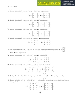
![Exercises 8.12
P =
− 1
√
2
0 1
2
1
2
0 − 1
√
2
−1
2
1
2
1
√
2
0 1
2
1
2
0 1
√
2
−1
2
1
2
, D =
0 0 0 0
0 0 0 0
0 0 −2 0
0 0 0 2
31. The given equation can be written as XT
AX = 24: [ x y ]
5 −1
−1 5
x
y
= 24. Using
λ1 = 6, λ2 = 4, K1 =
1
−1
, K2 =
1
1
, P =
1
√
2
1
√
2
− 1
√
2
1
√
2
and X = PX
we find
[ X Y ]
6 0
0 4
X
Y
= 24 or 6X2
+ 4Y 2
= 24.
The conic section is an ellipse. Now from X
= PT
X we see that the XY -coordinates of (1, −1) and (1, 1)
are (
√
2 , 0) and (0,
√
2 ), respectively. From this we conclude that the X-axis and Y -axis are as shown in the
accompanying figure.
32. The given equation can be written as XT
AX = 288: [ x y ]
13 −5
−5 13
x
y
= 288. Using
λ1 = 8, λ2 = 18, K1 =
1
1
, K2 =
−1
1
, P =
1
√
2
− 1
√
2
1
√
2
1
√
2
and X = PX
we find
[ X Y ]
8 0
0 18
X
Y
= 288 or 8X2
+ 18Y 2
= 288.
The conic section is an ellipse. Now from X
= PT
X we see that the XY -coordinates of (1, 1) and (1, −1) are
(
√
2 , 0) and (0, −
√
2 ), respectively. From this we conclude that the X-axis and Y -axis are as shown in the
accompanying figure.
33. The given equation can be written as XT
AX = 20: [ x y ]
−3 4
4 3
x
y
= 20. Using
λ1 = 5, λ2 = −5, K1 =
1
2
, K2 =
−2
1
, P =
1
√
5
− 2
√
5
2
√
5
1
√
5
and X = PX
we find
[ X Y ]
5 0
0 −5
X
Y
= 20 or 5X2
− 5Y 2
= 20.
The conic section is a hyperbola. Now from X
= PT
X we see that the XY -coordinates of (1, 2) and (−2, 1)
are (
√
5 , 0) and (0,
√
5 ), respectively. From this we conclude that the X-axis and Y -axis are as shown in the
accompanying figure.
34. The given equation can be written as XT
AX = 288:
[ x y ]
16 12
12 9
x
y
+ [ −3 4 ]
x
y
= 0.
Using λ1 = 25, λ2 = 0, K1 =
4
3
, K2 =
−3
4
, P =
4
5
3
5
3
5 −4
5
and X = PX
we find
[ X Y ]
25 0
0 0
X
Y
+ [ 0 5 ]
X
Y
= 0 or 25X2
+ 5Y = 0.
360](https://image.slidesharecdn.com/advancedengineeringmathematicssolutionsmanual-230807162553-1916df96/85/Advanced-Engineering-Mathematics-Solutions-Manual-pdf-360-320.jpg)

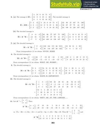
![Exercises 8.13
From correspondence (1) we obtain: DAD I NEED MONEY TODAY.
12. (a) MT
=
22 8 19 27 21 3 3 27 21 18 21
13 3 21 22 3 25 27 6 7 14 23
2 27 21 7 27 5 21 17 2 25 7
(b) BT
= M =
1 1 0
1 0 1
1 1 −1
=
37 38 61 56 51 33 51 50 30 57 51
24 35 40 34 48 8 24 44 23 43 28
11 −24 0 15 −24 20 6 −11 5 −11 16
(c) BA−1
= B
−1 1 1
2 −1 −1
1 0 −1
= M
13. (a) B
=
15 22 20 8 23 6 21 22
10 22 18 23 25 2 23 25
3 26 26 14 23 16 26 12
(b) Using correspondence (1) the encoded message is: OVTHWFUVJVRWYBWYCZZNWPZL.
(c) M
A−1
B
=
1 4 −3
2 3 −2
−2 −4 3
B
=
46 32 14 58 54 −34 35 86
54 58 42 57 75 −14 59 95
−61 −54 −34 −66 −77 28 −56 −108
M = M
mod 27 =
19 5 14 4 0 20 8 5
0 4 15 3 21 13 5 14
20 0 20 15 4 1 25 0
.
Using correspondence (1) the encoded message is: SEND THE DOCUMENT TODAY.
Exercises 8.14
1. [ 0 1 1 0 ] 2. [ 1 1 1 1 ]
3. [ 0 0 0 1 1 ] 4. [ 1 0 1 0 0 ]
5. [ 1 0 1 0 1 0 0 1 ] 6. [ 0 1 1 0 1 0 1 0 ]
7. [ 1 0 0 ] 8. [ 0 0 1 ]
9. Parity error 10. [ 1 0 1 0 ]
11. [ 1 0 0 1 1 ] 12. Parity error
364](https://image.slidesharecdn.com/advancedengineeringmathematicssolutionsmanual-230807162553-1916df96/85/Advanced-Engineering-Mathematics-Solutions-Manual-pdf-364-320.jpg)
![Exercises 8.14
In Problems 13-18 D = [ c1 c2 c3 ] and P =
1 1 0 1
1 0 1 1
0 1 1 1
.
13. DT
= P [ 1 1 1 0 ]
T
= [ 0 0 0 ]
T
; C = [ 0 0 1 0 1 1 0 ]
14. DT
= P [ 0 0 1 1 ]
T
= [ 1 0 0 ]
T
; C = [ 1 0 0 0 0 1 1 ]
15. DT
= P [ 0 1 0 1 ]
T
= [ 0 1 0 ]
T
; C = [ 0 1 0 0 1 0 1 ]
16. DT
= P [ 0 0 0 1 ]
T
= [ 1 1 1 ]
T
; C = [ 1 1 0 1 0 0 1 ]
17. DT
= P [ 0 1 1 0 ]
T
= [ 1 1 0 ]
T
; C = [ 1 1 0 0 1 1 0 ]
18. DT
= P [ 1 1 0 0 ]
T
= [ 0 1 1 ]
T
; C = [ 0 1 1 1 1 0 0 ]
In Problems 19-28 W represents the correctly decoded message.
19. S = HRT
= H [ 0 0 0 0 0 0 0 ] = [ 0 0 0 ]
T
; a code word. W = [ 0 0 0 0 ]
20. S = HRT
= H [ 1 1 0 0 0 0 0 ] = [ 0 1 1 ]
T
; not a code word. The error is in the third bit.
W = [ 1 0 0 0 ]
21. S = HRT
= H [ 1 1 0 1 1 0 1 ] = [ 1 0 1 ]
T
; not a code word. The error is in the fifth bit.
W = [ 0 0 0 1 ]
22. S = HRT
= H [ 0 1 0 1 0 1 0 ] = [ 0 0 0 ]
T
; a code word. W = [ 0 0 1 0 ]
23. S = HRT
= H [ 1 1 1 1 1 1 1 ] = [ 0 0 0 ]
T
; a code word. W = [ 1 1 1 1 ]
24. S = HRT
= H [ 1 1 0 0 1 1 0 ] = [ 0 0 0 ]
T
; a code word. W = [ 0 1 1 0 ]
25. S = HRT
= H [ 0 1 1 1 0 0 1 ] = [ 0 1 0 ]
T
; not a code word. The error is in the second bit.
W = [ 1 0 0 1 ]
26. S = HRT
= H [ 1 0 0 1 0 0 1 ] = [ 0 1 0 ]
T
; not a code word. The error is in the second bit.
W = [ 0 0 0 1 ]
27. S = HRT
= H [ 1 0 1 1 0 1 1 ] = [ 1 1 1 ]
T
; not a code word. The error is in the seventh bit.
W = [ 1 0 1 0 ]
28. S = HRT
= H [ 0 0 1 0 0 1 1 ] = [ 0 1 0 ]
T
; not a code word. The error is in the second bit.
W = [ 1 0 1 1 ]
29. (a) 27
= 128
(b) 24
= 16
(c) [ 0 0 0 0 0 0 0 ], [ 1 1 0 1 0 0 1 ], [ 0 1 0 1 0 1 0 ], [ 1 0 0 0 0 1 1 ],
[ 1 0 0 1 1 0 0 ], [ 0 1 0 0 1 0 1 ], [ 1 1 0 0 1 1 0 ], [ 0 0 0 1 1 1 1 ],
[ 1 1 1 0 0 0 0 ], [ 0 0 1 1 0 0 1 ], [ 1 0 1 1 0 1 0 ], [ 0 1 1 0 0 1 1 ],
[ 0 1 1 1 1 0 0 ], [ 1 0 1 0 1 0 1 ], [ 0 0 1 0 1 1 0 ], [ 1 1 1 1 1 1 1 ]
30. (a) c4 = 0, c3 = 1, c2 = 1, c1 = 0; [ 0 1 1 0 0 1 1 0 ]
(b) H =
0 0 0 0 1 1 1 1
0 0 1 1 0 0 1 1
0 1 0 1 0 1 0 1
1 1 1 1 1 1 1 1
(c) S = HRT
= H [ 0 0 1 1 1 1 0 0 ]
T
= [ 0 0 0 0 ]
T
365](https://image.slidesharecdn.com/advancedengineeringmathematicssolutionsmanual-230807162553-1916df96/85/Advanced-Engineering-Mathematics-Solutions-Manual-pdf-365-320.jpg)
![Exercises 8.15
Exercises 8.15
1. We have YT
= [ 1 2 3 2 ] and AT
=
2 3 4 5
1 1 1 1
.
Now AT
A =
54 14
14 4
and (AT
A)−1
=
1
20
4 −14
−14 54
so X = (AT
A)−1
AT
Y =
2
5
3
5
and the least squares line is y = 0.4x + 0.6.
2. We have YT
= [ −1 3 5 7 ] and AT
=
0 1 2 3
1 1 1 1
.
Now AT
A =
14 6
6 4
and (AT
A)−1
=
1
20
4 −6
−6 14
so X = (AT
A)−1
AT
Y =
13
5
−2
5
and the least squares line is y = 2.6x − 0.4.
3. We have YT
= [ 1 1.5 3 4.5 5 ] and AT
=
1 2 3 4 5
1 1 1 1 1
.
Now AT
A =
55 15
15 5
and (AT
A)−1
=
1
50
5 −15
−15 55
so X = (AT
A)−1
AT
Y =
1.1
−0.3
and the least squares line is y = 1.1x − 0.3.
4. We have YT
= [ 0 1.5 3 4.5 5 ] and AT
=
0 2 3 4 5
1 1 1 1 1
.
Now AT
A =
54 14
14 5
and (AT
A)−1
=
1
74
5 −14
−14 54
so X = (AT
A)−1
AT
Y =
1.06757
−0.189189
and the least squares line is y = 1.06757x − 0.189189.
5. We have YT
= [ 2 3 5 5 9 8 10 ] and AT
=
0 1 2 3 4 5 6
1 1 1 1 1 1 1
.
Now AT
A =
91 21
21 7
and (AT
A)−1
=
1
196
7 −21
−21 91
so X = (AT
A)−1
AT
Y =
19
14
27
14
and the least squares line is y = 1.35714x + 1.92857.
6. We have YT
= [ 2 2.5 1 1.5 2 3.2 5 ] and AT
=
1 2 3 4 5 6 7
1 1 1 1 1 1 1
.
Now AT
A =
140 28
28 7
and (AT
A)−1
=
1
196
7 −28
−28 140
so X = (AT
A)−1
AT
Y =
0.407143
0.828571
and the least squares line is y = 0.407143x + 0.828571.
366](https://image.slidesharecdn.com/advancedengineeringmathematicssolutionsmanual-230807162553-1916df96/85/Advanced-Engineering-Mathematics-Solutions-Manual-pdf-366-320.jpg)
![Exercises 8.16
7. We have YT
= [ 220 200 180 170 150 135 ] and AT
=
20 40 60 80 100 120
1 1 1 1 1 1
.
Now AT
A =
36400 420
420 6
and (AT
A)−1
=
1
42000
6 −420
−420 36400
so X = (AT
A)−1
AT
Y =
−117
140
703
3
and the least squares line is v = −0.835714T + 234.333. At T = 140,
v ≈ 117.333 and at T = 160, v ≈ 100.619.
8. We have YT
= [ 0.47 0.90 2.0 3.7 7.5 15 ] and AT
=
400 450 500 550 600 650
1 1 1 1 1 1
.
Now AT
A =
1697500 3150
3150 6
and (AT
A)−1
=
1
262500
6 −3150
−3150 1697500
so X = (AT
A)−1
AT
Y =
0.0538
−23.3167
and the least squares line is R = 0.0538T − 23.3167. At T = 700,
R ≈ 14.3433.
Exercises 8.16
In Problems 1-5 we use the fact that the element τij in the transfer matrix T is the rate of transfer from compartment
j to compartment i, and the fact that the sum of each column in T is 1.
1. (a) The initial state and the transfer matrix are
X0 =
90
60
and T =
0.8 0.4
0.2 0.6
.
(b) We have
X1 = TX0 =
0.8 0.4
0.2 0.6
90
60
=
96
54
and
X2 = TX1 =
0.8 0.4
0.2 0.6
96
54
=
98.4
51.6
.
(c) From TX̂ − X̂ = (T − I)X̂ = 0 and the fact that the system is closed we obtain
−0.2x1 + 0.4x2 = 0
x1 + x2 = 150.
The solution is x1 = 100, x2 = 50, so the equilibrium state is X̂ =
100
50
.
2. (a) The initial state and the transfer matrix are
X0 =
100
200
150
and T =
0.7 0 0.5
0.3 0.8 0
0 0.2 0.5
.
367](https://image.slidesharecdn.com/advancedengineeringmathematicssolutionsmanual-230807162553-1916df96/85/Advanced-Engineering-Mathematics-Solutions-Manual-pdf-367-320.jpg)
![Year Phytoplankton Water Zooplankton
0 0.00 100.00 0.00
1 2.00 97.00 1.00
2 3.70 94.26 2.04
3 5.14 91.76 3.10
4 6.36 89.47 4.17
5 7.39 87.37 5.24
6 8.25 85.46 6.30
7 8.97 83.70 7.33
8 9.56 82.10 8.34
9 10.06 80.62 9.32
10 10.46 79.28 10.26
11 10.79 78.04 11.17
12 11.06 76.90 12.04
Chapter 8 Review Exercises
5. (a) The initial state and the transfer matrix are
X0 =
0
100
0
and T =
0.88 0.02 0
0.06 0.97 0.05
0.06 0.01 0.95
.
(b)
6. From TX̂ = 1X̂ we see that the equilibrium state vector X̂ is the eigenvector of the transfer matrix T corre-
sponding to the eigenvalue 1. It has the properties that its components add up to the sum of the components
of the initial state vector.
Chapter 8 Review Exercises
1.
2 3 4
3 4 5
4 5 6
5 6 7
2. 4 × 3
3. AB =
3 4
6 8
; BA = [ 11 ]
4. A−1
= −
1
2
4 −2
−3 1
=
−2 1
3
2 −1
2
5. False; consider A =
1 0
0 1
and B =
0 1
1 0
6. True
7. det 1
2 A = 1
2
3
(5) = 5
8 ; det(−AT
) = (−1)3
(5) = −5
8. det AB−1
= det A/ det B = 6/2 = 3
9. 0
10. det C = (−1)3
/ det B = −1/103
(2) = −1/2000
11. False; an eigenvalue can be 0.
369](https://image.slidesharecdn.com/advancedengineeringmathematicssolutionsmanual-230807162553-1916df96/85/Advanced-Engineering-Mathematics-Solutions-Manual-pdf-369-320.jpg)
![Chapter 8 Review Exercises
12. True
13. True
14. True, since complex roots of real polynomials occur in conjugate pairs.
15. False; if the characteristic equation of an n×n matrix has repeated roots, there may not be n linearly independent
eigenvectors.
16. True
17. True
18. True
19. False; A is singular and thus not orthogonal.
20. True
21. A = 1
2 (A + AT
) + 1
2 (A − AT
) where 1
2 (A + AT
) is symmetric and 1
2 (A − AT
) is skew-symmetric.
22. Since det A2
= (det A)2
≥ 0 and det
0 1
1 0
= −1, there is no A such that A2
=
0 1
1 0
.
23. (a)
1 1
−1 −1
is nilpotent.
(b) Since det An
= (det A)n
= 0 we see that det A = 0 and A is singular.
24. (a) σxσy =
i 0
0 −i
= −σyσx; σxσz =
0 −1
1 0
= −σzσx; σyσz =
0 i
i 0
= −σzσy
(b) We first note that for anticommuting matrices AB = −BA, so C = 2AB. Then Cxy =
2i 0
0 −2i
,
Cyz =
0 2i
2i 0
, and Czx =
0 2
−2 0
.
25.
5 −1 1 −9
2 4 0 27
1 1 5 9
R13
−
−
−
−
−
−→
1 1 5 9
2 4 0 27
5 −1 1 −9
row
−
−
−
−
−
−→
operations
1 1 5 9
0 1 −5 9
2
0 0 1 1
2
row
−
−
−
−
−
−→
operations
1 0 0 −1
2
0 1 0 7
0 0 1 1
2
.
The solution is X = [ −1
2 7 1
2 ]
T
.
26.
1 1 1 6
1 −2 3 2
2 0 −3 3
row
−
−
−
−
−
−→
operations
1 1 1 6
0 1 −2
3
4
3
0 0 1 1
row
−
−
−
−
−
−→
operations
1 0 0 3
0 1 0 2
0 0 1 1
.
The solution is x1 = 3, x2 = 2, x3 = 1.
27. Multiplying the second row by abc we obtain the third row. Thus the determinant is 0.
28. Expanding along the first row we see that the result is an expression of the form ay + bx2
+ cx + d = 0, which
is a parabola since, in this case a = 0 and b = 0. Letting x = 1 and y = 2 we note that the first and second
rows are the same. Similarly, when x = 2 and y = 3, the first and third rows are the same; and when x = 3
and y = 5, the first and fourth rows are the same. In each case the determinant is 0 and the points lie on the
parabola.
29. 4(−2)(3)(−1)(2)(5) = 240
30. (−3)(6)(9)(1) = −162
370](https://image.slidesharecdn.com/advancedengineeringmathematicssolutionsmanual-230807162553-1916df96/85/Advanced-Engineering-Mathematics-Solutions-Manual-pdf-370-320.jpg)
![Chapter 8 Review Exercises
31. Since
1 −1 1
5 1 −1
1 2 1
= 18 = 0, the system has only the trivial solution.
32. Since
1 −1 −1
5 1 −1
1 2 1
= 0, the system has infinitely many solutions.
33. From x1I2 + x2HNO3 → x3HIO3 + x4NO2 + x5H2O we obtain the system 2x1 = x3, x2 = x3 + 2x5, x2 = x4,
3x2 = 3x3 +2x4 +x5. Letting x4 = x2 in the fourth equation we obtain x2 = 3x3 +x5. Taking x1 = t we see that
x3 = 2t, x2 = 2t + 2x5, and x2 = 6t + x5. From the latter two equations we get x5 = 4t. Taking t = 1 we have
x1 = 1, x2 = 10, x3 = 2, x4 = 10, and x5 = 4. The balanced equation is I2 +10HNO3 → 2HIO3 +10NO2 +4H2O.
34. From x1Ca + x2H3PO4 → x3Ca3P2O8 + x4H2 we obtain the system x1 = 3x3, 3x2 = 2x4, x2 = 2x3, 4x2 = 8x3.
Letting x3 = t we see that x1 = 3t, x2 = 2t, and x4 = 3t. Taking t = 1 we obtain the balanced equation
3Ca + 2H3PO4 → Ca3P2O8 + 3H2.
35. det A = −84, det A1 = 42, det A2 = −21, det A3 = −56; x1 =
42
−84
= −
1
2
, x2 =
−21
−84
=
1
4
, x3 =
−56
−84
=
2
3
36. det = 4, det A1 = 16, det A2 = −4, det A3 = 0; x1 =
16
4
= 4, x2 =
−4
4
= −1, x3 =
0
4
= 0
37. det A = cos2
θ + sin2
θ, det A1 = X cos θ − Y sin θ, det A2 = Y cos θ + X sin θ;
x1 = X cos θ − Y sin θ, y = Y cos θ + X sin θ
38. (a) i1 − i2 − i3 − i4 = 0, i2R1 = E, i2R1 − i3R2 = 0, i3R2 − i4R3 = 0
(b) det A =
1 −1 −1 −1
0 R1 0 0
0 R1 −R2 0
0 0 R2 −R3
= R1R2R3;
det A1 =
0 −1 −1 −1
E R1 0 0
0 R1 −R2 0
0 0 R2 −R3
= −E[−R2R3 − R1(R3 + R2)] = E(R2R3 + R1R3 + R1R2);
i1 =
det A1
det A
=
E(R2R3 + R1R3 + R1R2)
R1R2R3
= E
1
R1
+
1
R2
+
1
R3
39. AX = B is
2 3 −1
1 −2 0
−2 0 1
x1
x2
x3
=
6
−3
9
. Since A−1
= −
1
3
−2 −3 −2
−1 0 −1
−4 −6 −7
, we have
X = A−1
B =
7
5
23
.
40. (a) A−1
B =
3
2 −1
4 −9
4
−1 1
2
3
2
1
2 −1
4 −1
4
1
1
1
=
−1
1
0
(b) A−1
B =
3
2 −1
4 −9
4
−1 1
2
3
2
1
2 −1
4 −1
4
−2
1
3
=
−10
7
−2
371](https://image.slidesharecdn.com/advancedengineeringmathematicssolutionsmanual-230807162553-1916df96/85/Advanced-Engineering-Mathematics-Solutions-Manual-pdf-371-320.jpg)
![Chapter 8 Review Exercises
41. From the characteristic equation λ2
− 4λ − 5 = 0 we see that the eigenvalues are λ1 = −1 and λ2 = 5. For
λ1 = −1 we have 2k1 +2k2 = 0, 4k14k2 = 0 and K1 =
−1
1
. For λ2 = 5 we have −4k1 +2k2 = 0, 4k1 −2k2 = 0
and K2 =
1
2
.
42. From the characteristic equation λ2
= 0 we see that the eigenvalues are λ1 = λ2 = 0. For λ1 = λ2 = 0 we have
4k1 = 0 and K1 =
0
1
is a single eigenvector.
43. From the characteristic equation −λ3
+ 6λ2
+ 15λ + 8 = −(λ + 1)2
(λ − 8) = 0 we see that the eigenvalues are
λ1 = λ2 = −1 and λ3 = 8. For λ1 = λ2 = −1 we have
4 2 4 0
2 1 2 0
4 2 4 0
row
−
−
−
−
−
−→
operations
1 1
2 1 0
0 0 0 0
0 0 0 0
.
Thus K1 = [ 1 −2 0 ]
T
and K2 = [ 1 0 −1 ]
T
. For λ3 = 8 we have
−5 2 4 0
2 −8 2 0
4 2 −5 0
row
−
−
−
−
−
−→
operations
1 −2
5 −4
5 0
0 1 −1
2 0
0 0 0 0
.
Thus K3 = [ 2 1 2 ]
T
.
44. From the characteristic equation −λ3
+18λ2
−99λ+162 = −(λ−9)(λ−6)(λ−3) = 0 we see that the eigenvalues
are λ1 = 9, λ2 = 6, and λ3 = 3. For λ1 = 9 we have
−2 −2 0 0
−2 −3 2 0
0 2 −4 0
row
−
−
−
−
−
−→
operations
1 1 0 0
0 1 −2 0
0 0 0 0
.
Thus K1 = [ −2 2 1 ]
T
. For λ2 = 6 we have
1 −2 0 0
−2 0 2 0
0 2 −1 0
row
−
−
−
−
−
−→
operations
1 −2 0 0
0 1 −1
2 0
0 0 0 0
.
Thus K2 = [ 2 1 2 ]
T
. For λ3 = 3 we have
4 −2 0 0
−2 3 2 0
0 2 2 0
row
−
−
−
−
−
−→
operations
1 −1
2 0 0
0 1 1 0
0 0 0 0
.
Thus K3 = [ 1 2 −2 ]
T
.
45. From the characteristic equation −λ3
− λ2
+ 21λ + 45 = −(λ + 3)2
(λ − 5) = 0 we see that the eigenvalues are
λ1 = λ2 = −3 and λ3 = 5. For λ1 = λ2 = −3 we have
1 2 −3 0
2 4 −6 0
−1 −2 3 0
row
−
−
−
−
−
−→
operations
1 2 −3 0
0 0 0 0
0 0 0 0
.
Thus K1 = [ −2 1 0 ]
T
and K2 = [ 3 0 1 ]
T
. For λ3 = 5 we have
−7 2 −3 0
2 −4 −6 0
−1 −2 −5 0
row
−
−
−
−
−
−→
operations
1 −2
7
3
7 0
0 1 2 0
0 0 0 0
.
372](https://image.slidesharecdn.com/advancedengineeringmathematicssolutionsmanual-230807162553-1916df96/85/Advanced-Engineering-Mathematics-Solutions-Manual-pdf-372-320.jpg)
![Chapter 8 Review Exercises
Thus K3 = [ −1 −2 1 ]
T
.
46. From the characteristic equation −λ3
+ λ2
+ 2λ = −λ(λ + 1)(λ − 2) = 0 we see that the eigenvalues are λ1 = 0,
λ2 = −1, and λ3 = 2. For λ1 = 0 we have k3 = 0, 2k1 + 2k2 + k3 = 0 and K1 = [ 1 −1 0 ]
T
. For λ2 = −1 we
have
1 0 0 0
0 1 1 0
2 2 2 0
row
−
−
−
−
−
−→
operations
1 0 0 0
0 1 1 0
0 0 0 0
.
Thus K2 = [ 0 1 −1 ]
T
. For λ3 = 2 we have
−2 0 0 0
0 −2 1 0
2 2 −1 0
row
−
−
−
−
−
−→
operations
1 0 0 0
0 1 −1
2 0
0 0 0 0
.
Thus K3 = [ 0 1 2 ]
T
.
47. Let X1 = [ a b c ]
T
be the first column of the matrix. Then XT
1 [ − 1
√
2
0 1
√
2
]
T
= 1
√
2
(c − a) = 0 and
XT
1 [ 1
√
3
1
√
3
1
√
3
]
T
= 1
√
3
(a + b + c) = 0. Also XT
1 X1 = a2
+ b2
+ c2
= 1. We see that c = a and b = −2a from
the first two equations. Then a2
+ 4a2
+ a2
= 6a2
= 1 and a = 1
√
6
. Thus X1 = [ 1
√
6
− 2
√
6
1
√
6
]
T
.
48. (a) Eigenvalues are λ1 = λ2 = 0 and λ3 = 5 with corresponding eigenvectors K1 = [ 0 1 0 ]
T
, K2 =
[ 2 0 1 ]
T
, and K3 = [ −1 0 2 ]
T
. Since K1 = 1, K2 =
√
5 , and K3 =
√
5 , we have
P =
0 2
√
5
− 1
√
5
1 0 0
0 1
√
5
2
√
5
and P−1
= PT
=
0 1 0
2
√
5
0 1
√
5
− 1
√
5
0 2
√
5
.
(b) P−1
AP =
0 0 0
0 0 0
0 0 5
49. We identify A =
1 3
2
3
2 1
. Eigenvalues are λ1 = −1
2 and λ2 = 5
2 so D =
−1
2 0
0 5
2
and the equation becomes
[ X Y ] D
X
Y
= −1
2 X2
+ 5
2 Y 2
= 1. The graph is a hyperbola.
50. We measure years in units of 10, with 0 corresponding to 1890. Then Y = [ 63 76 92 106 123 ]
T
and
A =
0 1 2 3 4
1 1 1 1 1
T
, so AT
A =
30 10
10 5
. Thus
X = (AT
A)−1
AT
Y =
1
50
5 −10
−10 30
AT
Y =
15
62
,
and the least squares line is y = 15t + 62. At t = 5 (corresponding to 1940) we have y = 137. The error in the
predicted population is 5 million or 3.7%.
51. The encoded message is
B = AM =
10 1
9 1
19 1 20 5 12 12 9 20 5 0 12 1 21
14 3 8 5 4 0 15 14 0 6 18 9 0
=
204 13 208 55 124 120 105 214 50 6 138 19 210
185 12 188 50 112 108 96 194 45 6 126 18 189
.
373](https://image.slidesharecdn.com/advancedengineeringmathematicssolutionsmanual-230807162553-1916df96/85/Advanced-Engineering-Mathematics-Solutions-Manual-pdf-373-320.jpg)
![Chapter 8 Review Exercises
52. The encoded message is
B = AM =
10 1
9 1
19 5 3 0 1 7 14 20 0 1 18
18 22 19 0 20 21 5 19 0 1 13
=
208 72 49 0 30 91 145 219 0 11 193
189 67 46 0 29 84 131 199 0 10 175
.
53. The decoded message is
M = A−1
B =
−3 2 −1
1 0 0
2 −1 1
19 0 15 14 0 20
35 10 27 53 1 54
5 15 −3 48 2 39
=
8 5 12 16 0 9
19 0 15 14 0 20
8 5 0 23 1 25
.
From correspondence (1) we obtain: HELP IS ON THE WAY.
54. The decoded message is
M = A−1
B =
−3 2 −1
1 0 0
2 −1 1
5 2 21
27 17 40
21 13 −2
=
18 15 19
5 2 21
4 0 0
.
From correspondence (1) we obtain: ROSEBUD .
55. (a) The parity is even so the decoded message is [ 1 1 0 0 1 ]
(b) The parity is odd; there is a parity error.
56. From
c1
c2
c3
1 1 0 1
1 0 1 1
0 1 1 1
1
0
0
1
=
0
0
1
we obtain the codeword [ 0 0 1 1 0 0 1 ].
374](https://image.slidesharecdn.com/advancedengineeringmathematicssolutionsmanual-230807162553-1916df96/85/Advanced-Engineering-Mathematics-Solutions-Manual-pdf-374-320.jpg)
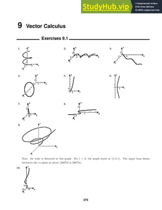
![Exercises 9.1
11. x = t, y = t, z = t2
+ t2
= 2t2
; r(t) = ti + tj + 2t2
k
12. x = t, y = 2t, z = ±
√
t2 + 4t2 + 1 = ±
√
5t2 − 1 ; r(t) = ti + 2tj ±
√
5t2 − 1 k
13. x = 3 cos t, z = 9 − 9 cos2
t = 9 sin2
t, y = 3 sin t; r(t) = 3 cos ti + 3 sin tj + 9 sin2
tk
14. x = sin t, z = 1, y = cos t; r(t) = sin ti + cos tj + k
15. r(t) =
sin 2t
t
i + (t − 2)5
j +
ln t
1/t
k. Using L’Hôpital’s Rule,
lim
t→0+
r(t) =
2 cos 2t
1
i + (t − 2)5
j +
1/t
−1/t2
k
= 2i − 32j.
16. (a) limt→α[−4r1(t) + 3r2(t)] = −4(i − 2j + k) + 3(2i + 5j + 7k) = 2i + 23j + 17k
(b) limt→α r1(t) · r2(t) = (i − 2j + k) · (2i + 5j + 7k) = −1
17. r
(t) =
1
t
i −
1
t2
j; r
(t) = −
1
t2
i +
2
t3
j
18. r
(t) = −t sin t, 1 − sin t; r
(t) = −t cos t − sin t, − cos t
376](https://image.slidesharecdn.com/advancedengineeringmathematicssolutionsmanual-230807162553-1916df96/85/Advanced-Engineering-Mathematics-Solutions-Manual-pdf-376-320.jpg)
![Exercises 9.1
19. r
(t) = 2te2t
+ e2t
, 3t2
, 8t − 1; r
(t) = 4te2t
+ 4e2t
, 6t, 8
20. r
(t) = 2ti + 3t2
j +
1
1 + t2
k; r
(t) = 2i + 6tj −
2t
(1 + t2)2
k
21. r
(t) = −2 sin ti + 6 cos tj
r
(π/6) = −i + 3
√
3 j
22. r
(t) = 3t2
i + 2tj
r
(−1) = 3i − 2j
23. r
(t) = j −
8t
(1 + t2)2
k
r
(1) = j − 2k
24. r
(t) = −3 sin ti + 3 cos tj + 2k
r
(π/4) =
−3
√
2
2
i +
3
√
2
2
j + 2k
25. r(t) = ti +
1
2
t2
j +
1
3
t3
k; r(2) = 2i + 2j +
8
3
k; r
(t) = i + tj + t2
k; r
(2) = i + 2j + 4k
Using the point (2, 2, 8/3) and the direction vector r
(2), we have x = 2 + t, y = 2 + 2t, z = 8/3 + 4t.
26. r(t) = (t3
−t)i+
6t
t + 1
j+(2t+1)2
k; r(1) = 3j+9k; r
(t) = (3t2
−1)i+
6
(t + 1)2
j+(8t+4)k; r
(1) = 2i+
3
2
j+12k.
Using the point (0, 3, 9) and the direction vector r
(1), we have x = 2t, y = 3 + 3
2 t, z = 9 + 12t.
27.
d
dt
[r(t) × r
(t)] = r(t) × r
(t) + r
(t) × r
(t) = r(t) × r
(t)
28.
d
dt
[r(t) · (tr(t))] = r(t) ·
d
dt
(tr(t)) + r
(t) · (tr(t)) = r(t) · (tr
(t) + r(t)) + r
(t) · (tr(t))
= r(t) · (tr
(t)) + r(t) · r(t) + r
(t) · (tr(t)) = 2t(r(t) · r
(t)) + r(t) · r(t)
29.
d
dt
[r(t) · (r
(t) × r
(t))] = r(t) ·
d
dt
(r
(t) × r
(t)) + r
(t) · (r
(t) × r
(t))
= r(t) · (r
(t) × r
(t) + r
(t) × r
(t)) + r
(t) · (r
(t) × r
(t))
= r(t) · (r
(t) × r
(t))
30.
d
dt
[r1(t) × (r2(t) × r3(t))] = r1(t) ×
d
dt
(r2(t) × r3(t)) + r
1(t) × (r2(t) × r3(t))
= r1(t) × (r2(t) × r
3(t) + r
2(t) × r3(t)) + r
1(t) × (r2(t) × r3(t))
= r1(t) × (r2(t) ×r
3(t)) + r1(t) ×(r
2(t) ×r3(t)) + r1(t) ×(r2(t) ×r3(t))
31.
d
dt
r1(2t) + r2
1
t
= 2r
1(2t) −
1
t2
r
2
1
t
377](https://image.slidesharecdn.com/advancedengineeringmathematicssolutionsmanual-230807162553-1916df96/85/Advanced-Engineering-Mathematics-Solutions-Manual-pdf-377-320.jpg)
![Exercises 9.1
32.
d
dt
[t3
r(t2
)] = t3
(2t)r
(t2
) + 3t2
r(t2
) = 2t4
r
(t2
) + 3t2
r(t2
)
33.
2
−1
r(t) dt =
2
−1
t dt
i +
2
−1
3t2
dt
j +
2
−1
4t3
dt
k =
1
2
t2
2
−1
i + t3
2
−1
j + t4
2
−1
k =
3
2
i + 9j + 15k
34.
4
0
r(t) dt =
4
0
√
2t + 1 dt
i +
4
0
−
√
t dt
j +
4
0
sin πt dt
k
=
1
3
(2t + 1)3/2
4
0
i −
2
3
t3/2
4
0
j −
1
π
cos πt
4
0
k =
26
3
i −
16
3
j
35.
r(t) dt =
tet
dt
i +
−e−2t
dt
j +
tet2
dt
k
= [tet
− et
+ c1]i +
1
2
e−2t
+ c2
j +
1
2
et2
+ c3
k = et
(t − 1)i +
1
2
e−2t
j +
1
2
et2
k + c,
where c = c1i + c2j + c3k.
36.
r(t) dt =
1
1 + t2
dt
i +
t
1 + t2
dt
j +
t2
1 + t2
dt
k
= [tan−1
t + c1]i +
1
2
ln(1 + t2
) + c2
j +
1 −
1
1 + t2
dt
k
= [tan−1
t + c1]i +
1
2
ln(1 + t2
) + c2
j + [t − tan−1
t + c3]k
= tan−1
ti +
1
2
ln(1 + t2
)j + (t − tan−1
t)k + c,
where c = c1i + c2j + c3k.
37. r(t) =
r
(t) dt =
6 dt
i +
6t dt
j +
3t2
dt
k = [6t + c1]i + [3t2
+ c2]j + [t3
+ c3]k
Since r(0) = i − 2j + k = c1i + c2j + c3k, c1 = 1, c2 = −2, and c3 = 1. Thus,
r(t) = (6t + 1)i + (3t2
− 2)j + (t3
+ 1)k.
38. r(t) =
r
(t) dt =
t sin t2
dt
i +
− cos 2t dt
j = −[
1
2
cos t2
+ c1]i + [−
1
2
sin 2t + c2]j
Since r(0) = 3
2 i = (−1
2 + c1)i + c2j, c1 = 2 and c2 = 0. Thus,
r(t) =
−
1
2
cos t2
+ 2
i −
1
2
sin 2tj.
39. r
(t) =
r
(t) dt =
12t dt
i +
−3t−1/2
dt
j +
2 dt
k = [6t2
+ c1]i + [−6t1/2
+ c2]j + [2t + c3]k
Since r
(1) = j = (6 + c1)i + (−6 + c2)j + (2 + c3)k, c1 = −6, c2 = 7, and c3 = −2. Thus,
r
(t) = (6t2
− 6)i + (−6t1/2
+ 7)j + (2t − 2)k.
r(t) =
r
(t) dt =
(6t2
− 6) dt
i +
(−6t1/2
+ 7) dt
j +
(2t − 2) dt
k
= [2t3
− 6t + c4]i + [−4t3/2
+ 7t + c5]j + [t2
− 2t + c6]k.
Since
r(1) = 2i − k = (−4 + c4)i + (3 + c5)j + (−1 + c6)k,
c4 = 6, c5 = −3, and c6 = 0. Thus,
r(t) = (2t3
− 6t + 6)i + (−4t3/2
+ 7t − 3)j + (t2
− 2t)k.
378](https://image.slidesharecdn.com/advancedengineeringmathematicssolutionsmanual-230807162553-1916df96/85/Advanced-Engineering-Mathematics-Solutions-Manual-pdf-378-320.jpg)
![Exercises 9.1
40. r
(t) =
r
(t) dt =
sec2
t dt
i +
cos t dt
j +
− sin t dt
k
= [tan t + c1]i + [sin t + c2]j + [cos t + c3]k
Since r
(0) = i + j + k = c1i + c2j + (1 + c3)k, c1 = 1, c2 = 1, and c3 = 0. Thus,
r
(t) = (tan t + 1)i + (sin t + 1)j + cos tk.
r(t) =
r
(t) dt =
(tan t + 1) dt
i +
(sin t + 1) dt
j +
cos t dt
k
= [ln | sec t| + t + c4]i + [− cos t + t + c5]j + [sin t + c6]k.
Since r(0) = −j + 5k = c4i + (−1 + c5)j + c6k, c4 = 0, c5 = 0, and c6 = 5. Thus,
r(t) = (ln | sec t| + t)i + (− cos t + t)j + (sin t + 5)k.
41. r
(t) = −a sin ti + a cos tj + ck; r
(t) = (−a sin t)2 + (a cos t)2 + c2 =
√
a2 + c2
s =
2π
0
a2 + c2 dt = a2 + c2 t
2π
0
= 2π a2 + c2
42. r
(t) = i + (cos t − t sin t)j + (sin t + t cos t)k
r
(t) = 12 + (cos t − t sin t)2 + (sin t + t cos t)2 =
√
2 + t2
s =
π
0
2 + t2 dt =
t
2
2 + t2 + ln t + 2 + t2
π
0
=
π
2
2 + π2 + ln(π + 2 + π2 ) − ln
√
2
43. r
(t) = (−2et
sin 2t + et
cos 2t)i + (2et
cos 2t + et
sin 2t)j + et
k
r
(t) = 5e2t cos2 2t + 5e2t sin2
2t + e2t =
√
6e2t =
√
6 et
s =
3π
0
√
6 et
dt =
√
6 et
3π
0
=
√
6 (e3π
− 1)
44. r
(t) = 3i + 2
√
3 tj + 2t2
k; r
(t) = 32 + (2
√
3 t)2 + (2t2)2 =
√
9 + 12t2 + 4t4 = 3 + 2t2
s =
1
0
(3 + 2t2
) dt = (3t +
2
3
t3
)
1
0
= 3 +
2
3
=
11
3
45. r
(t) = −a sin ti + a cos tj; r
(t) = a2 sin2
t + a2 cos2 t = a, a 0; s =
t
0
a du = at
r(s) = a cos(s/a)i + a sin(s/a)j; r
(s) = − sin(s/a)i + cos(s/a)j
r
(s) = sin2
(s/a) + cos2(s/a) = 1
46. r
(s) = −
2
√
5
sin(s/
√
5 )i +
2
√
5
cos(s/
√
5 )j +
1
√
5
k
r
(s) =
4
5
sin2
(s/
√
5 ) +
4
5
cos2(s/
√
5 ) +
1
5
=
4
5
+
1
5
= 1
47. Since
d
dt
(r · r) =
d
dt
r 2
=
d
dt
c2
= 0 and
d
dt
(r · r) = r · r
+ r
· r = 2r · r
, we have r · r
= 0. Thus,
r
is perpendicular to r.
48. Since r(t) is the length of r(t), r(t) = c represents a curve lying on a sphere of radius c centered at the
origin.
379](https://image.slidesharecdn.com/advancedengineeringmathematicssolutionsmanual-230807162553-1916df96/85/Advanced-Engineering-Mathematics-Solutions-Manual-pdf-379-320.jpg)
![Exercises 9.1
49. Let r1(t) = x(t)i + y(t)j. Then
d
dt
[u(t)r1(t)] =
d
dt
[u(t)x(t)i + u(t)y(t)j] = [u(t)x
(t) + u
(t)x(t)]i + [u(t)y
(t) + u
(t)y(t)]j
= u(t)[x
(t)i + y
(t)j] + u
(t)[x(t)i + y(t)j] = u(t)r
1(t) + u
(t)r1(t).
50. Let r1(t) = x1(t)i + y1(t)j and r2(t) = x2(t)i + y2(t)j. Then
d
dt
[r1(t) · r2(t)] =
d
dt
[x1(t)x2(t) + y1(t)y2(t)] = x1(t)x
2(t) + x
1(t)x2(t) + y1(t)y
2(t) + y
1(t)y2(t)
= [x1(t)x
2(t) + y1(t)y
2(t)] + [x
1(t)x2(t) + y
1(t)y2(t)] = r1(t) · r
2(t) + r
1(t) · r2(t).
51.
d
dt
[r1(t) × r2(t)] = lim
h→0
r1(t + h) × r2(t + h) − r1(t) × r2(t)
h
= lim
h→0
r1(t + h) × r2(t + h) − r1(t + h) × r2(t) + r1(t + h) × r2(t) − r1(t) × r2(t)
h
= lim
h→0
r1(t + h) × [r2(t + h) − r2(t)]
h
+ lim
h→0
[r1(t + h) − r1(t)] × r2(t)
h
= r1(t) × lim
h→0
r2(t + h) − r2(t)
h
+ lim
h→0
r1(t + h) − r1(t)
h
× r2(t)
= r1(t) × r
2(t) + r
1(t) × r2(t)
52. Let v = ai + bj and r(t) = x(t)i + y(t)j. Then
b
a
v · r(t) dt =
b
a
[ax(t) + by(t)] dt = a
b
a
x(t) dt + b
b
a
y(t) dt = v ·
b
a
r(t) dt.
Exercises 9.2
1. v(t) = 2ti + t3
j; v(1) = 2i + j; v(1) =
√
4 + 1 =
√
5 ;
a(t) = 2i + 3t2
j; a(1) = 2i + 3j
2. v(t) = 2ti −
2
t3
j; v(1) = 2i − 2j; v(1) =
√
4 + 4 = 2
√
2 ;
a(t) = 2i +
6
t4
j; a(1) = 2i + 6j
3. v(t) = −2 sinh 2ti+2 cosh 2tj; v(0) = 2j; v(0) = 2;
a(t) = −4 cosh 2ti + 4 sinh 2tj; a(0) = −4i
4. v(t) = −2 sin ti + cos tj; v(π/3) = −
√
3 i +
1
2
j; v(π/3) = 3 + 1/4 =
√
13/2;
a(t) = −2 cos ti − sin tj; a(π/3) = −i −
√
3
2
j
380](https://image.slidesharecdn.com/advancedengineeringmathematicssolutionsmanual-230807162553-1916df96/85/Advanced-Engineering-Mathematics-Solutions-Manual-pdf-380-320.jpg)
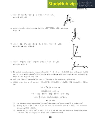
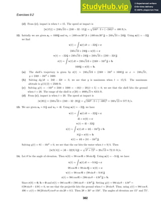
![Exercises 9.2
15. Let s be the initial speed. Then v(0) = s cos 45◦
i + s sin 45◦
j =
s
√
2
2
i +
s
√
2
2
j. Using a(t) = −32j, we have
v(t) =
a(t) dt = −32tj + c
s
√
2
2
i +
s
√
2
2
j = v(0) = c
v(t) =
s
√
2
2
i +
s
√
2
2
− 32t
j
r(t) =
s
√
2
2
ti +
s
√
2
2
t − 16t2
j + b.
Since r(0) = 0, b = 0 and
r(t) =
s
√
2
2
ti +
s
√
2
2
t − 16t2
j.
Setting y(t) = s
√
2 t/2 − 16t2
= t(s
√
2/2 − 16t) = 0 we see that the ball hits the ground when t =
√
2 s/32.
Thus, using x(t) = s
√
2 t/2 and the fact that 100 yd = 300 ft, 300 = x(t) =
s
√
2
2
(
√
2 s/32) =
s2
32
and
s =
√
9600 ≈ 97.98 ft/s.
16. Let s be the initial speed and θ the initial angle. Then v(0) = s cos θi + s sin θj. Using a(t) = −32j, we have
v(t) =
a(t) dt = −32tj + c
s cos θi + s sin θj = v(0) = c
v(t) = s cos θi + (s sin θ − 32t)j
r(t) = st cos θi + (st sin θ − 16t2
)j + b.
Since r(0) = 0, b = 0 and r(t) = st cos θi + (st sin θ − 16t2
)j. Setting y(t) = st sin θ − 16t2
= t(s sin θ − 16t) = 0,
we see that the ball hits the ground when t = (s sin θ)/16. Using x(t) = st cos θi, we see that the range of the
ball is
x
s sin θ
16
=
s2
sin θ cos θ
16
=
s2
sin 2θ
32
.
For θ = 30◦
, the range is s2
sin 60◦
/32 =
√
3 s2
/64 and for θ = 60◦
the range is s2
sin 120◦
/32 =
√
3 s2
/64. In
general, when the angle is 90◦
− θ the range is
[s2
sin 2(90◦
− θ)]/32 = s2
[sin(180◦
− 2θ)]/32 = s2
(sin 2θ)/32.
Thus, for angles θ and 90◦
− θ, the range is the same.
383](https://image.slidesharecdn.com/advancedengineeringmathematicssolutionsmanual-230807162553-1916df96/85/Advanced-Engineering-Mathematics-Solutions-Manual-pdf-383-320.jpg)
![Exercises 9.2
Since y
(t) = −g 0,
H = y
v0 sin θ
g
= −
1
2
g
v2
0 sin2
θ
g2
+ v0 sin θ
v0 sin θ
g
=
v2
0 sin2
θ
2g
is the maximum height. To find the range we solve y(t) = −1
2 gt2
+ (v0 sin θ)t = t(v0 sin θ − 1
2 gt) = 0. The
positive solution of this equation is t = (2v0 sin θ)/g. The range is thus
x(t) = (v0 cos θ)
2v0 sin θ
g
=
v2
0 sin 2θ
g
.
25. Letting r(t) = x(t)i + y(t)j + z(t)k, the equation dr/dt = v is equivalent to dx/dt = 6t2
x, dy/dt = −4ty2
,
dz/dt = 2t(z + 1). Separating variables and integrating, we obtain dx/x = 6t2
dt, dy/y2
= −4t dt, dz/(z + 1) =
2t dt, and ln x = 2t3
+ c1, −1/y = −2t2
+ c2, ln(z + 1) = t2
+ c3. Thus,
r(t) = k1e2t3
i +
1
2t2 + k2
j + (k3et2
− 1)k.
26. We require the fact that dr/dt = v. Then
dL
dt
=
d
dt
(r × p) = r ×
dp
dt
+
dr
dt
× p = τ
τ
τ + v × p = τ
τ
τ + v × mv = τ
τ
τ + m(v × v) = τ
τ
τ + 0 = τ
τ
τ.
27. (a) Since F is directed along r we have F = cr for some constant c. Then
τ
τ
τ = r × F = r × (cr) = c(r × r) = 0.
(b) If τ
τ
τ = 0 then dL/dt = 0 and L is constant.
28. (a) Using Problem 27, F = −k(Mm/r2
)u = ma. Then a = d2
r/dt = −k(M/r2
)u.
(b) Using u = r/r we have
r × r
= r × −k
M
r2
u = −
kM
r2
r × (
1
r
r)
= −
kM
r3
(r × r) = 0.
(c) From Theorem 9.4 (iv) we have
d
dt
(r × v) = r ×
dv
dt
+
dr
dt
× v = r × r
+ v × v = 0 + 0 = 0.
(d) Since r = ru we have c = r × v = ru × ru
= r2
(u × u
).
(e) Since u = (1/r)r is a unit vector, u · u = 1 and
d
dt
(u · u) = u ·
du
dt
+
du
dt
· u = 2u ·
du
dt
=
d
dt
(1) = 0.
Thus, u · u
= 0.
(f)
d
dt
(v × c) = v ×
dc
dt
+
dv
dt
× c = v × 0 + a × c = −
kM
r2
u × c = −
kM
r2
u × [r2
(u × u
)]
= −kM[u × (u × u
)] = −kM = −kM[(u · u
)u − (u · u)u
] by (10) of 7.4
= −kM[0 − u
] = kMu
= kM
du
dt
(g) Since
r · (v × c) = (r × v) · c by Problem 61 in 7.4
= c · c = c2
where c = c
385](https://image.slidesharecdn.com/advancedengineeringmathematicssolutionsmanual-230807162553-1916df96/85/Advanced-Engineering-Mathematics-Solutions-Manual-pdf-385-320.jpg)
![Exercises 9.2
and
(kMu + d) · r = (kMu + d) · ru = kMru · u + rd · u
= kMr + rd cos θ where d = d
we have c2
= kMr + rd cos θ or r =
c2
kM + d cos θ
=
c2
/kM
1 + (d/kM) cos θ
.
(h) First note that c 0 (otherwise there is no orbit) and d 0 (since the orbit is not a circle). We recognize
the equation in (g) to be that of a conic section with eccentricity e = d/kM. Since the orbit of the planet
is closed it must be an ellipse.
(i) At perihelion c = c = r × v = r0v0 sin(π/r) = r0v0. Since r is minimum at this point, we want the
denominator in the equation r0 = [c2
/kM]/[1 + (d/kM) cos θ] to be maximum. This occurs when θ = 0. In
this case
r0 =
r2
0v2
0/kM
1 + d/kM
and d = r0v2
0 − kM.
Exercises 9.3
1. r
(t) = −t sin ti + t cos tj + 2tk; |r
(t)| = t2 sin2
t + t2 cos2 t + 4t2 =
√
5 t;
T(t) = −
sin t
√
5
i +
cos t
√
5
j +
2
√
5
k
2. r
(t) = et
(− sin t + cos t)i + et
(cos t + sin t)j +
√
2 et
k,
|r
(t)| = [e2t
(sin2
t − 2 sin t cos t + cos2
t) + e2t
(cos2
t + 2 sin t cos t + sin2
t) + 2e2t
]1/2
=
√
4e2t = 2et
;
T(t) =
1
2
(− sin t + cos t)i +
1
2
(cos t + sin t)j +
√
2
2
k
3. We assume a 0. r
(t) = −a sin ti + a cos tj + ck; |r
(t)| = a2 sin2
t + a2 cos2 t + c2 =
√
a2 + c2 ;
T(t) = −
a sin t
√
a2 + c2
i +
a cos t
√
a2 + c2
j +
c
√
a2 + c2
k;
dT
dt
= −
a cos t
√
a2 + c2
i −
a sin t
√
a2 + c2
j,
dT
dt
=
a2 cos2 t
a2 + c2
+
a2 sin2
t
a2 + c2
=
a
√
a2 + c2
; N = − cos ti − sin tj;
B = T × N =
i j k
−
a sin t
√
a2 + c2
a cos t
√
a2 + c2
c
√
a2 + c2
− cos t − sin t 0
=
c sin t
√
a2 + c2
i −
c cos t
√
a2 + c2
j +
a
√
a2 + c2
k;
κ =
|dT/dt|
|r(t)|
=
a/
√
a2 + c2
√
a2 + c2
=
a
a2 + c2
4. r
(t) = i + tj + t2
k, r
(1) = i + j + k; |r
(t)| =
√
1 + t2 + t4 , |r
(1)| =
√
3 ;
T(t) = (1 + t2
+ t4
)−1/2
(i + tj + t2
k), T(1) =
1
√
3
(i + j + k);
dT
dt
= −
1
2
(1 + t2
+ t4
)−3/2
(2t + 4t3
)i + [(1 + t2
+ t4
)−1/2
−
t
2
(1 + t2
+ t4
)−3/2
(2t + 4t3
)]j
+ [2t(1 + t2
+ t4
)−1/2
−
t2
2
(1 + t2
+ t4
)−3/2
(2t + 4t3
)]k;
d
dt
T(1) = −
1
√
3
i +
1
√
3
k,
d
dt
T(1) =
1
3
+
1
3
=
√
2
√
3
; N(1) = −
1
√
2
(i − k);
386](https://image.slidesharecdn.com/advancedengineeringmathematicssolutionsmanual-230807162553-1916df96/85/Advanced-Engineering-Mathematics-Solutions-Manual-pdf-386-320.jpg)
![Exercises 9.3
16. v(t) = i + 2j + 4k, |v(t)| =
√
21 ; a(t) = 0; v · a = 0, v × a = 0, |v × a| = 0; aT = 0, aN = 0
17. v(t) = −a sin ti + b cos tj + ck, |v(t)| = a2 sin2
t + b2 cos2 t + c2 ; a(t) = −a cos ti − b sin tj;
v × a = bc sin ti − ac cos tj + abk, |v × a| = b2c2 sin2
t + a2c2 cos2 t + a2b2
κ =
|v × a|
|v|3
=
b2c2 sin2
t + a2c2 cos2 t + a2b2
(a2 sin2
t + b2 cos2 t + c2)3/2
;
18. (a) v(t) = −a sin ti + b cos tj, |v(t)| = a2 sin2
t + b2 cos2 t ; a(t) = −a cos ti − b sin tj;
v × a = abk; |v × a| = ab; κ =
ab
(a2 sin2
t + b2 cos2 t)3/2
(b) When a = b, |v(t)| = a, |v × a| = a2
, and κ = a2
/a3
= 1/a.
19. The equation of a line is r(t) = b + tc, where b and c are constant vectors.
v(t) = c, |v(t)| = |c|; a(t) = 0; v × a = 0, |v × a| = 0; κ = |v × a|/|v|3
= 0
20. v(t) = a(1 − cos t)i + a sin tj; v(π) = 2ai, |v(π)| = 2a; a(t) = a sin ti + a cos tj, a(π) = −aj;
|v × a| =
i j k
2a 0 0
0 −a 0
= −2a2
k; |v × a| = 2a2
; κ =
|v × a|
|v|3
=
2a2
8a3
=
1
4a
21. v(t) = f
(t)i + g
(t)j, |v(t)| = [f(t)]2 + [g(t)]2 ; a(t) = f
(t)i + g
(t)j;
v × a = [f
(t)g
(t) − g
(t)f
(t)]k, |v × a| = |f
(t)g
(t) − g
(t)f
(t)|;
κ =
|v × a|
|v|3
=
|f
(t)g
(t) − g
(t)f
(t)|
([f(t)]2 + [g(t)]2)3/2
22. For y = F(x), r(x) = xi + F(x)j. We identify f(x) = x and g(x) = F(x) in Problem 21. Then f
(x) = 1,
f
(x) = 0, g
(x) = F
(x), g
(x) = F
(x), and κ = |F
(x)|/(1 + [F
(x)]2
)3/2
.
23. F(x) = x2
, F(0) = 0, F(1) = 1; F
(x) = 2x, F
(0) = 0, F
(1) = 2; F
(x) = 2, F
(0) = 2, F
(1) = 2;
κ(0) =
2
(1 + 02)3/2
= 2; ρ(0) =
1
2
; κ(1) =
2
(1 + 22)3/2
=
2
5
√
5
≈ 0.18;
ρ(1) =
5
√
5
2
≈ 5.59; Since 2 2/5
√
5 , the curve is “sharper” at (0, 0).
24. F(x) = x3
, F(−1) = −1, F(1/2) = 1/8; F
(x) = 3x2
, F
(−1) = 3, F
(1/2) = 3/4; F
(x) = 6x,
F
(−1) = −6, F
(1/2) = 3; κ(−1) =
| − 6|
(1 + 32)3/2
=
6
10
√
10
=
3
5
√
10
≈ 0.19;
ρ(−1) =
5
√
10
3
≈ 5.27; κ(
1
2
) =
3
[1 + (3/4)2]3/2
=
3
125/64
=
192
125
≈ 1.54; ρ(
1
2
) =
125
192
≈ 0.65
Since 1.54 0.19, the curve is “sharper” at (1/2, 1/8).
25. At a point of inflection (x0, F(x0)), if F
(x0) exists then F
(x0) = 0. Thus, assuming that limx→x0
F
(x)
exists, F
(x) and hence κ is near 0 for x near x0.
26. We use the fact that T · N = 0 and T · T = N · N = 1. Then
|a(t)|2
= a · a = (aN N + aT T) · (aN N + aT T) = a2
N N · N + 2aN aT N · T + a2
T T · T = a2
N + a2
T .
388](https://image.slidesharecdn.com/advancedengineeringmathematicssolutionsmanual-230807162553-1916df96/85/Advanced-Engineering-Mathematics-Solutions-Manual-pdf-388-320.jpg)
![Exercises 9.4
17. zx =
2
√
x (3y2 + 1)
; zy = −
24y
√
x
(3y2 + 1)2
18. zx = 12x2
− 10x + 8; zy = 0
19. zx = −(x3
− y2
)−2
(3x2
) = −3x2
(x3
− y2
)−2
; zy = −(x3
− y2
)−2
(−2y) = 2y(x3
− y2
)−2
20. zx = 6(−x4
+ 7y2
+ 3y)5
(−4x3
) = −24x3
(−x4
+ 7y2
+ 3y)5
; zy = 6(−x4
+ 7y2
+ 3y)5
(14y + 3)
21. zx = 2(cos 5x)(− sin 5x)(5) = −10 sin 5x cos 5x; zy = 2(sin 5y)(cos 5y)(5) = 10 sin 5y cos 5y
22. zx = (2x tan−1
y2
)ex2
tan−1
y2
; zy =
2x2
y
1 + y4
ex2
tan−1
y2
23. fx = x(3x2
yex3
y
+ ex3
y
= (3x3
y + 1)ex3
y
; fy = x4
ex3
y
24. fθ = φ2
cos
θ
φ
1
φ
= φ cos
θ
φ
; fφ = φ2
cos
θ
φ
−
θ
φ2
+ 2φ sin
θ
φ
= −θ cos
θ
φ
+ 2φ sin
θ
φ
25. fx =
(x + 2y)3 − (3x − y)
(x + 2y)2
=
7y
(x + 2y)2
; fy =
(x + 2y)(−1) − (3x − y)(2)
(x + 2y)2
=
−7x
(x + 2y)2
26. fx =
(x2
− y2
)2
y − xy[2(x2
− y2
)2x]
(x2 − y2)4
=
−3x2
y − y3
(x2 − y2)3
;
fy =
(x2
− y2
)2
x − xy[2(x2
− y2
)(−2y)]
(x2 − y2)4
=
3xy2
+ x3
(x2 − y2)3
27. gu =
8u
4u2 + 5v3
; gv =
15v2
4u2 + 5v3
28. hr =
1
2s
√
r
+
√
s
r2
; hs = −
√
r
s2
−
1
2r
√
s
29. wx =
y
√
x
; wy = 2
√
x − y
1
z
ey/z
− ey/z
= 2
√
x −
y
z
+ 1
ey/z
; wz = −yey/z
−
y
z2
=
y2
z2
ey/z
30. wx = xy
1
x
+ (ln xz)y = y + y ln xz; wy = x ln xz; wz =
xy
z
31. Fu = 2uw2
− v3
− vwt2
sin(ut2
); Fv = −3uv2
+ w cos(ut2
);
Fx = 4(2x2
t)3
(4xt) = 16xt(2x2
t)3
= 128x7
t4
; Ft = −2uvwt sin(ut2
) + 64x8
t3
32. Gp = r4
s5
(p2
q3
)r4
s5
−1
(2pq3
) = 2pq3
r4
s5
(p2
q3
)r4
s5
−1
;
Gq = r4
s5
(p2
q3
)r4
s5
−1
(3p2
q2
) = 3p2
q2
r4
s5
(p2
q3
)r4
s5
−1
; Gr = (p2
q3
)r4
s5
(4r3
s5
) ln(p2
q3
);
Gs = (p2
q3
)r4
s5
(5r4
s4
) ln(p2
q3
)
33.
∂z
∂x
=
2x
x2 + y2
,
∂2
z
∂x2
=
(x2
+ y2
)2 − 2x(2x)
(x2 + y2)2
=
2y2
− 2x2
(x2 + y2)2
;
∂z
∂y
=
2y
x2 + y2
,
∂2
z
∂y2
=
(x2
+ y2
)2 − 2y(2y)
(x2 + y2)2
=
2x2
− 2y2
(x2 + y2)2
;
∂2
z
∂x2
+
∂2
z
∂y2
=
2y2
− 2x2
+ 2x2
− 2y2
(x2 + y2)2
= 0
34.
∂z
∂x
= ex2
−y2
(−2y sin 2xy) + 2xex2
−y2
cos 2xy
∂2
z
∂x2
= ex2
−y2
(−4y2
cos 2xy − 8xy sin 2xy + 4x2
cos 2xy + 2 cos 2xy)
∂z
∂y
= ex2
−y2
(−2x sin 2xy) − 2yex2
−y2
cos 2xy
∂2
z
∂y2
= ex2
−y2
(−4x2
cos 2xy + 8xy sin 2xy + 4y2
cos 2xy − 2 cos 2xy)
390](https://image.slidesharecdn.com/advancedengineeringmathematicssolutionsmanual-230807162553-1916df96/85/Advanced-Engineering-Mathematics-Solutions-Manual-pdf-390-320.jpg)
![Exercises 9.4
Adding the second partial derivatives gives
∂2
z
∂x2
+
∂2
z
∂y2
= [−4(y2
+ x2
) cos 2xy + 4(x2
+ y2
) cos 2xy] = 0.
35.
∂u
∂x
= cos at cos x,
∂2
u
∂x2
= − cos at sin x;
∂u
∂t
= −a sin at sin x,
∂2
u
∂t2
= −a2
cos at sin x;
a2 ∂2
u
∂x2
= a2
(− cos at sin x) =
∂2
u
∂t2
36.
∂u
∂x
= − sin(x + at) + cos(x − at),
∂2
u
∂x2
= − cos(x + at) − sin(x − at);
∂u
∂t
= −a sin(x + at) − a cos(x − at),
∂2
u
∂t2
= −a2
cos(x + at) − a2
sin(x − at);
a2 ∂2
u
∂x2
= −a2
cos(x + at) − a2
sin(x − at) =
∂2
u
∂t2
37.
∂C
∂x
= −
2x
kt
t−1/2
e−x2
/kt
,
∂2
C
∂x2
=
4x2
k2t2
t−1/2
e−x2
/kt
−
2
kt
t−1/2
e−x2
/kt
;
∂C
∂t
= t−1/2 x2
kt2
e−x2
/kt
−
t−3/2
2
e−x2
/kt
;
k
4
∂2
C
∂x2
=
x2
kt2
t−1/2
e−x2
/kt
−
t−1/2
2t
e−x2
/kt
=
∂C
∂t
38. (a) Pv = −k(T/V 2
)
(b) PV = kt, PVT = k, VT = k/P
(c) PV = kT, V = kTp, Tp = V/k
39. zx = v2
euv2
(3x2
) + 2uveuv2
(1) = 3x2
v2
euv2
+ 2uveuv2
; zy = v2
euv2
(0) + 2uveuv2
(−2y) = −4yuveuv2
40. zx = (2u cos 4v)(2xy3
) − (4u2
sin 4v)(3x2
) = 4xy3
u cos 4v − 12x2
u2
sin 4v
zy = (2u cos 4v)(3x2
y2
) − (4v2
sin 4v)(3y2
) = 6x2
y2
u cos 4v − 12y2
u2
sin 4v
41. zu = 4(4u3
) − 10y[2(2u − v)(2)] = 16u3
− 40(2u − v)y
zv = 4(−24v2
) − 10y[2(2u − v)(−1)] = −96v2
+ 20(2u − v)y
42. zu =
2y
(x + y)2
1
v
+
−2x
(x + y)2
−
v2
u2
=
2y
v(x + y)2
+
2xv2
u2(x + y)2
zv =
2y
(x + y)2
−
u
v2
+
−2x
(x + y)2
2v
u
= −
2yu
v2(x + y)2
−
4xv
u(x + y)2
43. wt =
3
2
(u2
+ v2
)1/2
(2u)(−e−t
sin θ) +
3
2
(u2
+ v2
)1/2
(2v)(−e−t
cos θ)
= −3u(u2
+ v2
)1/2
e−t
sin θ − 3v(u2
+ v2
)1/2
e−t
cos θ
wθ =
3
2
(u2
+ v2
)1/2
(2u)e−t
cos θ +
3
2
(u2
+ v2
)1/2
(2v)(−e−t
sin θ)
= 3u(u2
+ v2
)1/2
e−t
cos θ − 3v(u2
+ v2
)1/2
e−t
sin θ
44. wr =
v/2
√
uv
1 + uv
(2r) +
u/2
√
uv
1 + uv
(2rs2
) =
rv
√
uv (1 + uv)
+
rs2
u
√
uv (1 + uv)
ws =
v/2
√
uv
1 + uv
(−2s) +
u/2
√
uv
1 + uv
(2r2
s) =
−sv
√
uv (1 + uv)
+
r2
su
√
uv (1 + uv)
45. Ru = s2
t4
(ev2
) + 2rst4
(−2uve−u2
) + 4rs2
t3
(2uv2
eu2
v2
) = s2
t4
ev2
− 4uvrst4
e−u2
+ 8uv2
rs2
t3
eu2
v2
Rv = s2
t4
(2uvev2
) + 2rst4
(e−u2
) + 4rs2
t3
(2u2
veu2
v2
) = 2s2
t4
uvev2
+ 2rst4
e−u2
+ 8rs2
t3
u2
veu2
v2
46. Qx =
1
P
t2
√
1 − x2
+
1
q
1
t2
+
1
r
1/t
1 + (x/t)2
=
t2
p
√
1 − x2
+
1
qt2
+
t
r(t2 + x2)
391](https://image.slidesharecdn.com/advancedengineeringmathematicssolutionsmanual-230807162553-1916df96/85/Advanced-Engineering-Mathematics-Solutions-Manual-pdf-391-320.jpg)
![Exercises 9.4
Qt =
1
p
(2t sin−1
x) +
1
q
−
2x
t3
+
1
r
−x/t2
1 + (x/t)2
=
2t sin−1
x
p
−
2x
qt3
−
x
r(t2 + x2)
47. wt =
2x
2 x2 + y2
u
rs + tu
+
2y
2 x2 + y2
cosh rs
u
=
xu
x2 + y2 (rs + tu)
+
y cosh rs
u x2 + y2
wr =
2x
2 x2 + y2
s
rs + tu
+
2y
2 x2 + y2
st sinh rs
u
=
xs
x2 + y2 (rs + tu)
+
yst sinh rs
u x2 + y2
wu =
2x
2 x2 + y2
t
rs + tu
+
2y
2 x2 + y2
−t cosh rs
u2
=
xt
x2 + y2 (rs + tu)
−
yt cosh rs
u2 x2 + y2
48. sφ = 2pe3θ
+ 2q[− sin(φ + θ)] − 2rθ2
+ 4(2) = 2pe3θ
− 2q sin(φ + θ) − 2rθ2
+ 8
sθ = 2p(3φe3θ
) + 2q[− sin(φ + θ)] − 2r(2φθ) + 4(8) = 6pφe3θ
− 2q sin(φ + θ) − 4rφθ + 32
49.
dz
dt
=
2u
u2 + v2
(2t) +
2v
u2 + v2
(−2t−3
) =
4ut − 4vt−3
u2 + v2
50.
dz
dt
= (3u2
v − v4
)(−5e−5t
) + (u3
− 4uv3
)(5 sec 5t tan 5t) = −5(3u2
v − v4
)e−5t
+ 5(u3
− 4uv3
) sec 5t tan 5t
51.
dw
dt
= −3 sin(3u + 4v)(2) − 4 sin(3u + 4v)(−1); u(π) = 5π/2, v(π) = −5π/4
dw
dt π
= −6 sin
15π
2
− 5π + 4 sin
15π
2
− 5π = −2 sin
5π
2
= −2
52.
dw
dt
= yexy
−8
(2t + 1)2
+ xexy
(3); x(0) = 4, y(0) = 5;
dw
dt 0
= 5e20
(−8) + 4e20
(3) = −28e20
53. With x = r cos θ and y = r sin θ
∂u
∂r
=
∂u
∂x
∂x
∂r
+
∂u
∂y
∂y
∂r
=
∂u
∂x
cos θ +
∂u
∂y
sin θ
∂2
u
∂r2
=
∂2
u
∂x2
∂x
∂r
cos θ +
∂2
u
∂y2
∂y
∂r
sin θ =
∂2
u
∂x2
cos2
θ +
∂2
u
∂y2
sin2
θ
∂u
∂θ
=
∂u
∂x
∂x
∂θ
+
∂u
∂y
∂y
∂θ
=
∂u
∂x
(−r sin θ) +
∂u
∂y
(r cos θ)
∂2
u
∂θ2
=
∂u
∂x
(−r cos θ) +
∂2
u
∂x2
∂x
∂θ
(−r sin θ) +
∂u
∂y
(−r sin θ) +
∂2
u
∂y2
∂y
∂θ
(r cos θ)
= −r
∂u
∂x
cos θ + r2 ∂2
u
∂x2
sin2
θ − r
∂u
∂y
sin θ + r2 ∂2
u
∂y2
cos2
θ.
Using
∂2
u
∂x2
+
∂2
u
∂y2
= 0, we have
∂2
u
∂r2
+
1
r
∂u
∂r
+
1
r2
∂2
u
∂θ2
=
∂2
u
∂x2
cos2
θ +
∂2
u
∂y2
sin2
θ +
1
r
∂u
∂x
cos θ +
∂u
∂y
sin θ
+
1
r2
−r
∂u
∂x
cos θ + r2 ∂2
u
∂x2
sin2
θ − r
∂u
∂y
sin θ + r2 ∂2
u
∂y2
cos2
θ
=
∂2
u
∂x2
(cos2
θ + sin2
θ) +
∂2
u
∂y2
(sin2
θ + cos2
θ) +
∂u
∂x
1
r
cos θ −
1
r
cos θ
+
∂u
∂y
1
r
sin θ −
1
r
sin θ
=
∂2
u
∂x2
+
∂2
u
∂y2
= 0.
392](https://image.slidesharecdn.com/advancedengineeringmathematicssolutionsmanual-230807162553-1916df96/85/Advanced-Engineering-Mathematics-Solutions-Manual-pdf-392-320.jpg)
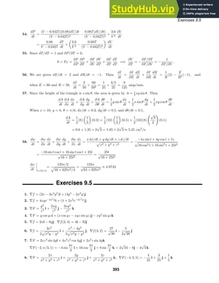

![Exercises 9.5
22. u = (−2i + 5j)/
√
29 ; ∇f = (3x2
− 5y)i − (5x − 2y)j; ∇f(1, 1) = −2i − 3j;
Duf(1, 1) =
4
√
29
−
15
√
29
= −
11
√
29
23. ∇f = 2e2x
sin yi + e2x
cos yj; ∇f(0, π/4) =
√
2 i +
√
2
2
j
The maximum Du is [(
√
2 )2
+ (
√
2/2)2
]1/2
= 5/2 in the direction
√
2 i + (
√
2/2)j.
24. ∇f = (xyex−y
+ yex−y
)i + (−xyex−y
+ xex−y
)j; ∇f(5, 5) = 30i − 20j
The maximum Du is [302
+ (−20)2
]1/2
= 10
√
13 in the direction 30i − 20j.
25. ∇F = (2x + 4z)i + 2z2
j + (4x + 4yz)k; ∇F(1, 2, −1) = −2i + 2j − 4k
The maximum Du is [(−2)2
+ 22
+ (−4)2
]1/2
= 2
√
6 in the direction −2i + 2j − 4k.
26. ∇F = yzi + xzj + xyk; ∇F(3, 1, −5) = −5i − 15j + 3k
The maximum Du is [(−5)2
+ (−15)2
+ 32
]1/2
=
√
259 in the direction −5i − 15j + 3k.
27. ∇f = 2x sec2
(x2
+ y2
)i + 2y sec2
(x2
+ y2
)j;
∇f( π/6 , π/6 ) = 2 π/6 sec2
(π/3)(i + j) = 8 π/6 (i + j)
The minimum Du is −8 π/6 (12
+ 12
)1/2
= −8 π/3 in the direction −(i + j).
28. ∇f = 3x2
i − 3y2
j; ∇f(2, −2) = 12i − 12j = 12(i − j)
The minimum Du is −12[12
+ (−1)2
]1/2
= −12
√
2 in the direction −(i − j) = −i + j.
29. ∇F =
√
z ey
2
√
x
i +
√
xz ey
j +
√
x
2
√
z
k; ∇F(16, 0, 9) =
3
8
i + 12j +
2
3
k. The minimum Du is
−[(3/8)2
+ 122
+ (2/3)2
]1/2
= −
√
83,281/24 in the direction −
3
8
i − 12j −
2
3
k.
30. ∇F =
1
x
i +
1
y
j −
1
z
k; ∇F(1/2, 1/6, 1/3) = 2i + 6j − 3k
The minimum Du is −[22
+ 62
+ (−3)2
]1/2
= −7 in the direction −2i − 6j + 3k.
31. Using implicit differentiation on 2x2
+ y2
= 9 we find y
= −2x/y. At (2, 1) the slope of the tangent line is
−2(2)/1 = −4. Thus, u = ±(i − 4j)/
√
17 . Now, ∇f = i + 2yj and ∇f(3, 4) = i + 8j. Thus,
Du = ±(1/
√
17 − 32
√
17 ) = ±31/
√
17 .
32. ∇f = (2x + y − 1)i + (x + 2y)j; Duf(x, y) =
2x + y − 1
√
2
+
x + 2y
√
2
=
3x + 3y − 1
√
2
Solving (3x + 3y − 1)/
√
2 = 0 we see that Du is 0 for all points on the line 3x + 3y = 1.
33. (a) Vectors perpendicular to 4i + 3j are ±(3i − 4j). Take u = ±
3
5
i −
4
5
j .
(b) u = (4i + 3j)/
√
16 + 9 =
4
5
i +
3
5
j
(c) u = −
4
5
i −
3
5
j
34. D−uf(a, b) = ∇f(a, b) · (−u) = −∇f(a, b) · u = −Duf(a, b) = −6
35. (a) ∇f = (3x2
− 6xy2
)i + (−6x2
y + 3y2
)j
Duf(x, y) =
3(3x2
− 6xy2
)
√
10
+
−6x2
y + 3y2
√
10
=
9x2
− 18xy2
− 6x2
y + 3y2
√
10
(b) F(x, y) =
3
√
10
(3x2
− 6xy2
− 2x2
y + y2
); ∇F =
3
√
10
[(6x − 6y2
− 4xy)i + (−12xy − 2x2
+ 2y)j]
395](https://image.slidesharecdn.com/advancedengineeringmathematicssolutionsmanual-230807162553-1916df96/85/Advanced-Engineering-Mathematics-Solutions-Manual-pdf-395-320.jpg)
![Exercises 9.5
DuF(x, y) =
3
√
10
3
√
10
(6x − 6y2
− 4xy) +
1
√
10
3
√
10
(−12xy − 2x2
+ 2y)
=
9
5
(3x − 3y2
− 2xy) +
3
5
(−6xy − x2
+ y) =
1
5
(27x − 27y2
− 36xy − 3x2
+ 3y)
36. ∇U =
Gmx
(x2 + y2)3/2
i +
Gmy
(x2 + y2)3/2
j =
Gm
(x2 + y2)3/2
(xi + yj)
The maximum and minimum values of DuU(x, y) are obtained when u is in the directions ∇U and −∇U,
respectively. Thus, at a point (x, y), not (0, 0), the directions of maximum and minimum increase in U are
xi + yj and −xi − yj, respectively. A vector at (x, y) in the direction ±(xi + yj) lies on a line through the origin.
37. ∇f = (3x2
− 12)i + (2y − 10)j. Setting |∇f| = [(3x2
− 12)2
+ (2y − 10)2
]1/2
= 0, we obtain 3x2
− 12 = 0 and
2y − 10 = 0. The points where |∇f| = 0 are (2, 5) and (−2, 5).
38. Let ∇f(a, b) = αi + βj. Then
Duf(a, b) = ∇f(a, b) · u =
5
13
α −
12
13
β = 7 and Dvf(a, b) = ∇f(a, b) · v =
5
13
α −
12
13
β = 3.
Solving for α and β, we obtain α = 13 and β = −13/6. Thus, ∇f(a, b) = 13i − (13/6)j.
39. ∇T = 4xi + 2yj; ∇T(4, 2) = 16i + 4j. The minimum change in temperature (that is, the maximum decrease
in temperature) is in the direction −∇T(4, 3) = −16i − 4j.
40. Let x(t)i + y(t)j be the vector equation of the path. At (x, y) on this curve, the direction of a tangent vector is
x
(t)i + y
(t)j. Since we want the direction of motion to be −∇T(x, y), we have x
(t)i + y
(t)j = −∇T(x, y) =
4xi + 2yj. Separating variables in dx/dt = 4x, we obtain dx/x = 4 dt, ln x = 4t + c1, and x = C1e4t
. Separating
variables in dy/dt = 2y, we obtain dy/y = 2 dt, ln y = 2t + c2, and y = C2e2t
. Since x(0) = 4 and y(0) = 2, we
have x = 4e4t
and y = 2e2t
. The equation of the path is 4e4t
i + 2e2t
j for t ≥ 0, or eliminating the parameter,
x = y2
, y ≥ 0.
41. Let x(t)i + y(t)j be the vector equation of the path. At (x, y) on this curve, the direction of a tangent vector
is x
(t)i + y
(t)j. Since we want the direction of motion to be ∇T(x, y), we have x
(t)i + y
(t)j = ∇T(x, y) =
−4xi − 2yj. Separating variables in dx/dt = −4x we obtain dx/x = −4 dt, ln x = −4t + c1 and x = C1e−4t
.
Separating variables in dy/dt = −2y we obtain dy/y = −2 dt, ln y = −2t + c2 and y = C2e−2t
. Since x(0) = 3
and y(0) = 4, we have x = 3e−4t
and y = 4e−2t
. The equation of the path is 3e−4t
i + 4e−2t
j, or eliminating the
parameter, 16x = 3y2
, y ≥ 0.
42. Substituting x = 0, y = 0, z = 1, and T = 500 into T = k/(x2
+ y2
+ z2
) we see that k = 500 and
T(x, y, z) = 500/(x2
+ y2
+ z2
) .
(a) u =
1
3
1, −2, −2 =
1
3
i −
2
3
j −
2
3
k
∇T = −
1000x
(x2 + y2 + z2)2
i −
1000y
(x2 + y2 + z2)2
j −
1000z
(x2 + y2 + z2)2
k
∇T(2, 3, 3) = −
500
121
i −
750
121
j −
750
121
k
DuT(2, 3, 3) =
1
3
−
500
121
−
2
3
−
750
121
−
2
3
−
750
121
=
2500
363
(b) The direction of maximum increase is ∇T(2, 3, 3) = −
500
121
i −
750
121
j −
750
121
k =
250
121
(−2i − 3j − 3k).
(c) The maximum rate of change of T is |∇T(2, 3, 3)| =
250
121
√
4 + 9 + 9 =
250
√
22
121
.
396](https://image.slidesharecdn.com/advancedengineeringmathematicssolutionsmanual-230807162553-1916df96/85/Advanced-Engineering-Mathematics-Solutions-Manual-pdf-396-320.jpg)
![Exercises 9.6
43. Since ∇f = fx(x, y)i + fy(x, y)j, we have ∂f/∂x = 3x2
+ y3
+ yexy
. Integrating, we obtain f(x, y) = x3
+ xy3
+
exy
+ g(y). Then fy = 3xy2
+ xexy
+ g
(y) = −2y2
+ 3xy2
+ xexy
. Thus, g
(y) = −2y2
, g(y) = −2
3 y3
+ c, and
f(x, y) = x3
+ xy3
+ exy
− 2
3 y3
+ C.
44. Let u = u1i + u2j and v = v1i + v2j. Dvf = (fxi + fyj) · v = v1fx + v2fy
DuDvf =
∂
∂x
(v1fx + v2fy)i +
∂
∂y
(v1fx + v2fy)j
· u = [(v1fxx + v2fyx)i + (v1fxy + v2fyy)j] · u
= u1v1fxx + u1v2fyx + u2v1fxy + u2v2fyy
Duf = (fxi + fyj) · u = u1fx + u2fy
DvDuf =
∂
∂x
(u1fx + u2fy)i +
∂
∂y
(u1fx + u2fy)j
· v = [(u1fxx + u2fyx)i + (u1fxy + u2fyy)j] · v
= u1v1fxx + u2v1fyx + u1v2fxy + u2v2fyy
Since the second partial derivatives are continuous, fxy = fyx and DuDvf = DvDuf. [Note that this result is
a generalization of fxy = fyx since DiDjf = fyx and DjDif = fxy.]
45. ∇(cf) =
∂
∂x
(cf)i +
∂
∂y
(cf)j = cfxi + cfyj = c(fxi + fyj) = c∇f
46. ∇(f + g) = (fx + gx)i + (fy + gy)j = (fxi + fyj) + (gxi + gyj) = ∇f + ∇g
47. ∇(fg) = (fgx + fxg)i + (fgy + fyg)j = f(gxi + gyj) + g(fxi + fyj) = f∇g + g∇f
48. ∇(f/g) = [(gfx − fgx)/g2
]i + [(gfy − fgy)/g2
]j = g(fxi + fyj)/g2
− f(gxi + gyj)/g2
= g∇f/g2
− f∇g/g2
= (g∇f − f∇g)/g2
49. ∇ × F =
i j k
∂/∂x ∂/∂y ∂/∂z
f1 f2 f3
=
∂f3
∂y
−
∂f2
∂z
i +
∂f1
∂z
−
∂f3
∂x
j +
∂f2
∂x
−
∂f1
∂y
k
Exercises 9.6
1. Since f(6, 1) = 4, the level curve is x − 2y = 4.
∇f = i − 2j; ∇f(6, 1) = i − 2j
2. Since f(1, 3) = 5, the level curve is y + 2x = 5x or y = 3x, x = 0.
∇f = −
y
x2
i +
1
x
j; ∇f(1, 3) = −3i + j
3. Since f(2, 5) = 1, the level curve is y = x2
+ 1.
∇f = −2xi + j; ∇f(2, 5) = −10i + j
4. Since f(−1, 3) = 10, the level curve is x2
+ y2
= 10.
∇f = 2xi + 2yj; ∇f(−1, 3) = −2i + 6j
5. Since f(−2, −3) = 2, the level curve is x2
/4 + y2
/9 = 2
or x2
/8 + y2
/18 = 1. ∇f =
x
2
i +
2y
9
j; ∇f(−2, −3) = −i −
2
3
j
397](https://image.slidesharecdn.com/advancedengineeringmathematicssolutionsmanual-230807162553-1916df96/85/Advanced-Engineering-Mathematics-Solutions-Manual-pdf-397-320.jpg)
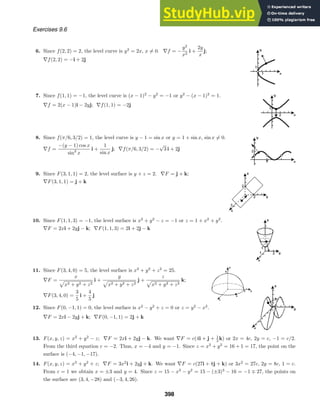
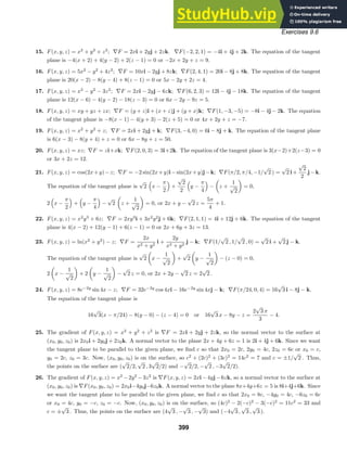
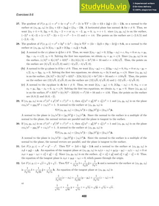
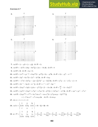
![Exercises 9.7
(a × ∇) × r =
i j k
a2
∂
∂z
− a3 a3
∂
∂x
− a1
∂
∂z
a1
∂
∂y
− a2
∂
∂x
x y z
= (−a1 − a1)i − (a2 + a2)j + (−a3 − a3)k = −2a
20. ∇ × (a × r) = (∇ · r)a − (∇ · a)r = (1 + 1 + 1)a − a1
∂
∂x
+ a2
∂
∂y
+ a3
∂
∂z
r = 3a − (a1i + a2j + a3k) = 2a
21. ∇ · (a × r) =
∂/∂x ∂/∂y ∂/∂z
a1 a2 a3
x y z
=
∂
∂x
(a2z − a3y) −
∂
∂y
(a1z − a3x) +
∂
∂z
(a1y − a2x) = 0
22. ∇ × r =
i j k
∂/∂x ∂/∂y ∂/∂z
x y z
= 0; a × (∇ × r) = a × 0 = 0
23. r × a =
i j k
x y z
a1 a2 a3
= (a3y − a2z)i − (a3x − a1z)j + (a2x − a1y)k; r · r = x2
+ y2
+ z2
∇ × [(r · r)a] =
i j k
∂/∂x ∂/∂y ∂/∂z
(r · r)a1 (r · r)a2 (r · r)a3
= (2ya3 − 2za2)i − (2xa3 − 2za1)j + (2xa2 − 2ya1)k = 2(r × a)
24. r · a = a1x + a2y + a3z; r · r = x2
+ y2
+ z2
; ∇ · [(r · r)a] = 2xa1 + 2ya2 + 2za3 = 2(r · a)
25. Let F = P(x, y, z)i + Q(x, y, z)j + R(x, y, z)k and G = S(x, y, z)i + T(x, y, z)j + U(x, y, z)k.
∇ · (F + G) = ∇ · [(P + S)i + (Q + T)j + (R + U)k] = Px + Sx + Qy + Ty + Rz + Uz
= (Px + Qy + Rz) + (Sx + Ty + Uz) = ∇ · F + ∇ · G
26. Let F = P(x, y, z)i + Q(x, y, z)j + R(x, y, z)k and G = S(x, y, z)i + T(x, y, z)j + U(x, y, z)k.
∇ × (F + G) =
i j k
∂/∂x ∂/∂y ∂/∂z
P + S Q + T R + U
= (Ry + Uy − Qz − Tz)i − (Rx + Ux − Pz − Sz)j + (Qx + Tx − Py − Sy)k
= (Ry − Qz)i − (Rx − Pz)j + (Qx − Py)k + (Uy − Tz)i − (Ux − Sz)j + (Tx − Sy)k
= ∇ × F + ∇ × G
27. ∇ · (fF) = ∇ · (fPi + fQj + fRk) = fPx + Pfx + fQy + Qfy + fRz + Rfz
= f(Px + Qy + Rz) + (Pfx + Qfy + Rfz) = f(∇ · F) + F · (∇f)
403](https://image.slidesharecdn.com/advancedengineeringmathematicssolutionsmanual-230807162553-1916df96/85/Advanced-Engineering-Mathematics-Solutions-Manual-pdf-403-320.jpg)
![Exercises 9.7
28. ∇ × (fF) =
i j k
∂/∂x ∂/∂y ∂/∂z
fP fQ fR
= (fRy + Rfy − fQz − Qfz)i − (fRx + Rfx − fPz − Pfz)j + (fQx + Qfx − fPy − Pfy)k
= (fRy − fQz)i − (fRx − fPz)j + (fQx − fPy)k + (Rfy − Qfz)i
− (Rfx − Pfz)j + (Qfx − Pfy)k
= f[(Ry − Qz)i − (Rx − Pz)j + (Qx − Py)k +
i j k
fx fy fz
P Q R
= f(∇ × F) + (∇f) × F
29. Assuming continuous second partial derivatives,
curl (grad f) = ∇ × (fxi + fyj + fzk) =
i j k
∂/∂x ∂/∂y ∂/∂z
fx fy fz
= (fzy − fyz)i − (fzx − fxz)j + (fyx − fxy)k = 0.
30. Assuming continuous second partial derivatives,
div (curl F) = ∇ · [(Ry − Qz)i − (Rx − Pz)j + (Qx − Py)k]
= (Ryx − Qzx − (Rxy − Pzy) + (Qxz − Pyz) = 0.
31. Let F = P(x, y, z)i + Q(x, y, z)j + R(x, y, z)k and G = S(x, y, z)i + T(x, y, z)j + U(x, y, z)k.
F × G =
i j k
P Q R
S T U
= (QU − RT)i − (PU − RS)j + (PT − QS)k
div (F × G) = (QUx + QxU − RTx − RxT) − (PUy + PyU − RSy − RyS) + (PTz + PzT − QSz − QzS)
= S(Ry − Qz) + T(Pz − Rx) + U(Qx − Py) − P(Uy − Tz) − Q(Sz − Ux) − R(Tx − Sy)
= G · (curl F) − F · (curl G)
32. Using Problems 26 and 29,
curl (curl F + grad f) = ∇ × (curl F + grad f) = ∇ × (curl F) + ∇ × (grad f)
= curl (curl F) + curl (grad f) = curl (curl F) + 0 = curl (curl F).
33. ∇ · ∇f = ∇ · (fxi + fyj + fzk) = fxx + fyy + fzz
34. Using Problem 27, ∇ · (f∇f) = f(∇ · ∇f) + ∇f · ∇f = f(∇2
f) + |∇f|2
.
35. curl F = −8yzi − 2zj − xk; curl (curl F) = 2i − (8y − 1)j + 8zk
36. (a) For F = Pi + Qj + Rk,
curl (curl F) = (Qxy − Pyy − Pzz + Rxz)i + (Ryz − Qzz − Qxx + Pyx)j
+ (Pzx − Rxx − Ryy + Qzy)k
and
404](https://image.slidesharecdn.com/advancedengineeringmathematicssolutionsmanual-230807162553-1916df96/85/Advanced-Engineering-Mathematics-Solutions-Manual-pdf-404-320.jpg)
![Exercises 9.7
−∇2
F + grad (div F) = −(Pxx + Pyy + Pzz)i − (Qxx + Qyy + Qzz)j − (Rxx + Ryy + Rzz)k
+ grad (Px + Qy + Rz)
= −Pxxi − Qyyj − Rzzk + (−Pyy − Pzz)i + (−Qxx − Qzz)j
+ (−Rxx − Ryy)k + (Pxx + Qyx + Rzx)i + (Pxy + Qyy + Rzy)j
+ (Pxz + Qyz + Rzz)k
= (−Pyy − Pzz + Qyx + Rzx)i + (−Qxx − Qzz + Pxy + Rzy)j
+ (−Rxx − Ryy + Pxz + Qyz)k.
Thus, curl (curl F) = −∇2
F + grad (div F).
(b) For F = xyi + 4yz2
j + 2xzk, ∇2
F = 0i + 8yj + 0k, div F = y + 4z2
+ 2x, and grad (div F) = 2i + j + 8zk.
Then curl (curl F) = −8yj + 2i + j + 8zk = 2i + (1 − 8y)j + 8zk.
37.
∂f
∂x
= −x(x2
+ y2
+ z2
)−3/2
∂f
∂y
= −y(x2
+ y2
+ z2
)−3/2
∂f
∂z
= −z(x2
+ y2
+ z2
)−3/2
∂2
f
∂x2
= 3x2
(x2
+ y2
+ z2
)−5/2
− (x2
+ y2
+ z2
)−3/2
∂2
f
∂y2
= 3y2
(x2
+ y2
+ z2
)−5/2
− (x2
+ y2
+ z2
)−3/2
∂2
f
∂z2
= 3z2
(x2
+ y2
+ z2
)−5/2
− (x2
+ y2
+ z2
)−3/2
Adding the second partial derivatives gives
∂2
f
∂x2
+
∂2
f
∂y2
+
∂2
f
∂z2
=
3(x2
+ y2
+ z2
)
(x2 + y2 + z2)5/2
− 3(x2
+ y2
+ z2
)−3/2
= 3(x2
+ y2
+ z2
)−3/2
− 3(x2
+ y2
+ z2
)−3/2
= 0
except when x = y = z = 0.
38. fx =
1
1 +
4y2
(x2 + y2 − 1)2
−
4xy
(x2 + y2 − 1)2
= −
4xy
(x2 + y2 − 1)2 + 4y2
fxx = −
[(x2
+ y2
− 1)2
+ 4y2
]4y − 4xy[4x(x2
+ y2
− 1)]
[(x2 + y2 − 1)2 + 4y2]2
=
12x4
y − 4y5
+ 8x2
y3
− 8x2
y − 8y3
− 4y
[(x2 + y2 − 1)2 + 4y2]2
fy =
1
1 +
4y2
(x2 + y2 − 1)2
2(x2
+ y2
− 1) − 4y2
(x2 + y2 − 1)2
=
2(x2
− y2
− 1)
(x2 + y2 − 1)2 + 4y2
fyy =
[(x2
+ y2
− 1)2
+ 4y2
](−4y) − 2(x2
− y2
− 1)[4y(x2
+ y2
− 1) + 8y]
[(x2 + y2 − 1)2 + 4y2]2
=
−12x4
y + 4y5
− 8x2
y3
+ 8x2
y + 8y3
+ 4y
[(x2 + y2 − 1)2 + 4y2]2
∇2
f = fxx + fyy = 0
405](https://image.slidesharecdn.com/advancedengineeringmathematicssolutionsmanual-230807162553-1916df96/85/Advanced-Engineering-Mathematics-Solutions-Manual-pdf-405-320.jpg)
![Exercises 9.7
39. curl F = −Gm1m2
i j k
∂/∂x ∂/∂y ∂/∂z
x/|r|3
y/|r|3
z/|r|3
= −Gm1m2[(−3yz/|r|5
+ 3yz/|r|5
)i − (−3xz/|r|5
+ 3xz/|r|5
)j + (−3xy/|r|5
+ 3xy/|r|5
)k]
= 0
div F = −Gm1m2
−2x2
+ y2
+ z2
|r|5/2
+
x2
− 2y2
+ z2
|r|5/2
+
x2
+ y2
− 2z2
|r|5/2
= 0
40.
1
2
curl v =
1
2
curl (ω
ω
ω × r) =
1
2
i j k
∂/∂x ∂/∂y ∂/∂z
ω2z − ω3y ω3x − ω1z ω1y − ω2x
=
1
2
[(ω1 + ω1)i − (−ω2 − ω2)j + (ω3 + ω3)k] = ω1i + ω2j + ω3k = ω
ω
ω
41. Using Problems 31 and 29,
∇ · F = div (∇f × ∇g) = ∇g · (curl ∇f) − ∇f · (curl ∇g) = ∇g · 0 − ∇f · 0 = 0.
42. Recall that a · (a × b) = 0. Then, using Problems 31, 29, and 28,
∇ · F = div (∇f × f∇g) = f∇g · (curl ∇f) − ∇f · (curl f∇g) = f∇g · 0 − ∇f · (∇ × f∇g)
= −∇f · [f(∇ × ∇g) + (∇f × ∇g)] = −∇f · [fcurl ∇g + (∇f × ∇g]
= −∇f · [f0 + (∇f × ∇g)] = −∇f · (∇f × ∇g) = 0.
43. (a) Expressing the vertical component of V in polar coordinates, we have
2xy
(x2 + y2)2
=
2r2
sin θ cos θ
r4
=
sin 2θ
r2
.
Similarly,
x2
− y2
(x2 + y2)2
=
r2
(cos2
θ − sin2
θ)
r4
=
cos 2θ
r2
.
Since limr→∞(sin 2θ)/r2
= limr→∞(cos 2θ)/r2
= 0, V ≈ Ai for r large or (x, y) far from the origin.
(b) Identifying P(x, y) = A
1 −
x2
− y2
(x2 − y2)2
, Q(x, y) = −
2Axy
(x2 + y2)2
, and R(x, y) = 0, we have
Py =
2Ay(3x2
− y2
)
(x2 + y2)3
, Qx =
2Ay(3x2
− y2
)
(x2 + y2)3
, and Pz = Qz = Rx = Ry = 0.
Thus, curl V = (Ry − Qz)i + (Pz − Rx)j + (Qx − Py)k = 0 and V is irrotational.
(c) Since Px =
2Ax(x2
− 3y2
)
(x2 + y2)3
, Qy =
2Ax(3y2
− x2
)
(x2 + y2)3
, and Rz = 0, ∇ · F = Px + Qy + Rz = 0 and V is
incompressible.
44. We first note that curl (∂H/∂t) = ∂(curl H)/∂t and curl (∂E/∂t) = ∂(curl E)/∂t. Then, from Problem 30,
−∇2
E = −∇2
E + 0 = −∇2
E + grad 0 = −∇2
E + grad (div E) = curl (curl E)
= curl −
1
c
∂H
∂t
= −
1
c
∂
∂t
curl H = −
1
c
∂
∂t
1
c
∂E
∂t
= −
1
c2
∂2
E
∂t
406](https://image.slidesharecdn.com/advancedengineeringmathematicssolutionsmanual-230807162553-1916df96/85/Advanced-Engineering-Mathematics-Solutions-Manual-pdf-406-320.jpg)
![Exercises 9.8
and ∇2
E = 1
c2 ∂2
E/∂t2
. Similarly,
−∇2
H = −∇2
H + grad (div H) = curl (curl H) = curl
1
c
∂E
∂t
=
1
c
∂
∂t
curl E
=
1
c
∂
∂t
−
1
c
∂H
∂t
= −
1
c2
∂2
H
∂t2
and ∇2
H =
1
c2
∂2
H/∂t2
.
45. We note that div F = 2xyz − 2xyz + 1 = 1 = 0. If F = curl G, then div (curl G) = div F = 1. But, by
Problem 30, for any vector field G, div (curl G) = 0. Thus, F cannot be the curl of G.
Exercises 9.8
1.
C
2xy dx =
π/4
0
2(5 cos t)(5 sin t)(−5 sin t) dt = −250
π/4
0
sin2
t cos t dt = −250
1
3
sin3
t
π/4
0
= −
125
√
2
6
C
2xy dy =
π/4
0
2(5 cos t)(5 sin t)(5 cos t) dt = 250
π/4
0
cos2
t sin t dt = 250 −
1
3
cos3
t
π/4
0
=
250
3
1 −
√
2
4
=
125
6
(4 −
√
2)
C
2xy ds =
π/4
0
2(5 cos t)(5 sin t) 25 sin2
t + 25 cos2 t dt = 250
π/4
0
sin t cos t dt
= 250
1
2
sin2
t
π/4
0
=
125
2
2.
C
(x3
+ 2xy2
+ 2x) dx =
1
0
[8t3
+ 2(2t)(t4
) + 2(2t)]2 dt = 2
1
0
(8t3
+ 4t5
+ 4t) dt
= 2 2t4
+
2
3
t6
+ 2t2
1
0
=
28
3
C
(x3
+ 2xy2
+ 2x) dy =
1
0
[8t3
+ 2(2t)(t4
) + 2(2t)]2t dt = 2
1
0
(8t4
+ 4t6
+ 4t2
) dt
= 2
8
5
t5
+
4
7
t7
+
4
3
t3
1
0
=
736
105
C
(x3
+ 2xy2
+ 2x) ds =
1
0
[8t3
+ 2(2t)(t4
) + 2(2t)] 4 + 4t2 dt = 8
1
0
t(1 + t2
)5/2
dt
= 8
1
7
(1 + t2
)7/2
1
0
=
8
7
(27/2
− 1)
3.
C
(3x2
+ 6y2
) dx =
0
−1
[3x2
+ 6(2x + 1)2
] dx =
0
−1
(27x2
+ 24x + 6) dx = (9x3
+ 12x2
+ 6x)
0
−1
= −(−9 + 12 − 6) = 3
C
(3x2
+ 6y2
) dy =
0
−1
[3x2
+ 6(2x + 1)2
]2 dx = 6
C
(3x2
+ 6y2
) ds =
0
−1
[3x2
+ 6(2x + 1)2
]
√
1 + 4 dx = 3
√
5
407](https://image.slidesharecdn.com/advancedengineeringmathematicssolutionsmanual-230807162553-1916df96/85/Advanced-Engineering-Mathematics-Solutions-Manual-pdf-407-320.jpg)
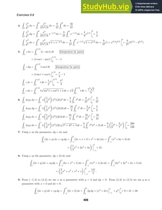
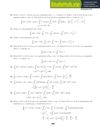
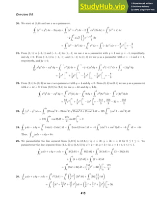

![Exercises 9.8
and
W =
C1
F1 · dr1 +
C2
F2 · dr2 +
C3
F3 · dr3
=
1
0
(6 + 4t)dt +
1
0
6tdt +
1
0
(−14 + 8t − 6 + 2t)dt
=
1
0
(−14 + 20t) dt = (−14t + 10t2
)
1
0
= −4.
34. F = t3
i + t4
j + t5
k; dr = 3t2
i + 2tj + k; W =
C
F · dr =
3
1
(3t5
+ 2t5
+ t5
) dt =
3
1
6t5
dt = t6
3
1
= 728
35. r = 3 cos ti + 3 sin tj, 0 ≤ t ≤ 2π; dr = −3 sin ti + 3 cos tj; F = ai + bj;
W =
C
F · dr =
2π
0
(−3a sin t + 3b cos t) dt = (3a cos t + 3b sin t)
2π
0
= 0
36. Let r = ti + tj + tk for 1 ≤ t ≤ 3. Then dr = i + j + k, and
F =
c
|r|3
(ti + tj + tk) =
ct
(
√
3t2 )3
(i + j + k) =
c
3
√
3 t2
(i + j + k),
W =
C
F · dr =
3
1
c
3
√
3 t2
(1 + 1 + 1) dt =
c
√
3
3
1
1
t2
dt =
c
√
3
−
1
t
3
1
=
c
√
3
−
1
3
+ 1 =
2c
3
√
3
.
37.
C1
y2
dx + xy dy =
1
0
(4t + 2)2
2 dt +
1
0
(2t + 1)(4t + 2)4 dt =
1
0
(64t2
+ 64t + 16) dt
=
64
3
t3
+ 32t2
+ 16t
1
0
=
64
3
+ 32 + 16 =
208
3
C2
y2
dx + xy dy =
√
3
1
4t4
(2t) dt +
√
3
1
2t4
(4t) dt =
√
3
1
16t5
dt =
8
3
t6
√
3
1
= 72 −
8
3
=
208
3
C3
y2
dx + xy dy =
e3
e
4(ln t)2 1
t
dt +
e3
e
2(ln t)2 2
t
dt =
e3
e
8
t
(ln t)2
dt =
8
3
(ln t)3
e3
e
=
8
3
(27 − 1) =
208
3
38.
C1
xy ds =
2
0
t(2t)
√
1 + 4 dt = 2
√
5
2
0
t2
dt = 2
√
5
1
3
t3
2
0
=
16
√
5
3
C2
xy ds =
2
0
t(t2
) 1 + 4t2 dt =
2
0
t3
1 + 4t2 dt u = 1 + 4t2
, du = 8t dt, t2
= 1
4 (u − 1)
=
17
1
1
4
(u − 1)u1/2 1
8
du =
1
32
17
1
(u3/2
− u1/2
) du =
1
32
2
5
u5/2
−
2
3
u3/2
17
1
=
391
√
17 + 1
120
C3
xy ds =
3
2
(2t − 4)(4t − 8)
√
4 + 16 dt = 16
√
5
3
2
(t − 2)2
dt = 16
√
5
1
3
(t − 2)3
3
2
=
16
√
5
3
C1 and C3 are different parameterizations of the same curve, while C1 and C2 are different curves.
39. Since v · v = v2
,
d
dt
v2
=
d
dt
(v · v) = v ·
dv
dt
+
dv
dt
· v = 2
dv
dt
· v. Then
W =
C
F · dr =
b
a
ma ·
dr
dt
dt = m
b
a
dv
dt
· v dt = m
b
a
1
2
d
dt
v2
dt
=
1
2
m(v2
)
b
a
=
1
2
m[v(b)]2
−
1
2
m[v(a)]2
.
412](https://image.slidesharecdn.com/advancedengineeringmathematicssolutionsmanual-230807162553-1916df96/85/Advanced-Engineering-Mathematics-Solutions-Manual-pdf-412-320.jpg)
![Exercises 9.9
40. We are given ρ = kx. Then
m =
C
ρ ds =
π
0
kx ds = k
π
0
(1 + cos t) sin2
t + cos2 t dt = k
π
0
(1 + cos t) dt
= k(t + sin t)
π
0
= kπ.
41. From Problem 40, m = kπ and ds = dt.
Mx =
C
yρ ds =
C
kxy ds = k
π
0
(1 + cos t) sin t dt = k − cos t +
1
2
sin2
t
π
0
= 2k
My =
C
xρ ds =
C
kx2
ds = k
π
0
(1 + cos t)2
dt = k
π
0
(1 + 2 cos t + cos2
t) dt
= k t + 2 sin t +
1
2
t +
1
4
sin 2t
π
0
=
3
2
kπ
x̄ = My/m =
3kπ/2
kπ
=
3
2
; ȳ = Mx/m =
2k
kπ
=
2
π
. The center of mass is (3/2, 2/π).
42. On C1, T = i and F · T = compTF ≈ 1. On C2, T = −j and F · T = compTF ≈ 2. On C3, T = −i and
F · T = compTF ≈ 1.5. Using the fact that the lengths of C1, C2, and C3 are 4, 5, and 5, respectively, we have
W =
C
F · T ds =
C1
F · T ds +
C2
F · T ds +
C3
F · T ds ≈ 1(4) + 2(5) + 1.5(5) = 21.5 ft-lb.
Exercises 9.9
1. (a) Py = 0 = Qx and the integral is independent of path. φx = x2
, φ =
1
3
x3
+ g(y),
φy = g
(y) = y2
, g(y) =
1
3
y3
, φ =
1
3
x3
+
1
3
y3
,
(2,2)
(0,0)
x2
dx + y2
dy =
1
3
(x3
+ y3
)
(2,2)
(0,0)
=
16
3
(b) Use y = x for 0 ≤ x ≤ 2.
(2,2)
(0,0)
x2
dx + y2
dy =
2
0
(x2
+ x2
) dx =
2
3
x3
2
0
=
16
3
2. (a) Py = 2x = Qx and the integral is independent of path. φx = 2xy, φ = x2
y + g(y),
φy = x2
+ g
(y) = x2
, g(y) = 0, φ = x2
y,
(2,4)
(1,1)
2xy dx + x2
dy = x2
y
(2,4)
(1,1)
= 16 − 1 = 15
(b) Use y = 3x − 2 for 1 ≤ x ≤ 2.
(2,4)
(1,1)
2xy dx + x2
dy =
2
1
[2x(3x − 2) + x2
(3)] dx =
2
1
(9x2
− 4x) dx = (3x3
− 2x2
)
2
1
= 15
3. (a) Py = 2 = Qx and the integral is independent of path. φx = x + 2y, φ =
1
2
x2
+ 2xy + g(y),
φy = 2x + g
(y) = 2x − y, g(y) = −
1
2
y2
, φ =
1
2
x2
+ 2xy −
1
2
y2
,
(3,2)
(1,0)
(x + 2y) dx + (2x − y) dy =
1
2
x2
+ 2xy −
1
2
y2
(3,2)
(1,0)
= 14
413](https://image.slidesharecdn.com/advancedengineeringmathematicssolutionsmanual-230807162553-1916df96/85/Advanced-Engineering-Mathematics-Solutions-Manual-pdf-413-320.jpg)
![Exercises 9.9
(b) Use y = x − 1 for 1 ≤ x ≤ 3.
(3,2)
(1,0)
(x + 2y) dx + (2x − y) dy =
3
1
[x + 2(x − 1) + 2x − (x − 1) dx
=
3
1
(4x − 1) dx = (2x2
− x)
3
1
= 14
4. (a) Py = − cos x sin y = Qx and the integral is independent of path. φx = cos x cos y,
φ = sin x cos y + g(y), φy = − sin x sin y + g
(y) = 1 − sin x sin y, g(y) = y, φ = sin x cos y + y,
(π/2,0)
(0,0)
cos x cos y dx + (1 − sin x sin y) dy = (sin x cos y + y)
(π/2,0)
(0,0)
= 1
(b) Use y = 0 for 0 ≤ x ≤ π/2.
(π/2,0)
(0,0)
cos x cos y dx + (1 − sin x sin y) dy =
π/2
0
cos x dx = sin x
π/2
0
= 1
5. (a) Py = 1/y2
= Qx and the integral is independent of path. φx = −
1
y
, φ = −
x
y
+g(y), φy =
x
y2
+g
(x) =
x
y2
,
g(y) = 0, φ = −
x
y
,
(4,4)
(4,1)
−
1
y
dx +
x
y2
dy = (−
x
y
)
(4,4)
(4,1)
= 3
(b) Use x = 4 for 1 ≤ y ≤ 4.
(4,4)
(4,1)
−
1
y
dx +
x
y2
dy =
4
1
4
y2
dy = −
4
y
4
1
= 3
6. (a) Py = −xy(x2
+ y2
)−3/2
= Qx and the integral is independent of path. φx =
x
x2 + y2
,
φ = x2 + y2 + g(y), φy =
y
x2 + y2
+ g
(y) =
y
x2 + y2
, g(y) = 0, φ = x2 + y2 ,
(3,4)
(1,0)
x dx + y dy
x2 + y2
= x2 + y2
(3,4)
(1,0)
= 4
(b) Use y = 2x − 2 for 1 ≤ x ≤ 3.
(3,4)
(1,0)
x dx + y dy
x2 + y2
=
3
1
x + (2x − 2)2
x2 + (2x − 2)2
dx =
3
1
5x − 4
√
5x2 − 8x + 4
= 5x2 − 8x + 4
3
1
= 4
7. (a) Py = 4xy = Qx and the integral is independent of path. φx = 2y2
x − 3, φ = x2
y2
− 3x + g(y),
φy = 2x2
y + g
(y) = 2x2
y + 4, g(y) = 4y, φ = x2
y2
− 3x + 4y,
(3,6)
(1,2)
(2y2
x − 3) dx + (2yx2
+ 4) dy = (x2
y2
− 3x + 4y)
(3,6)
(1,2)
= 330
(b) Use y = 2x for 1 ≤ x ≤ 3.
(3,6)
(1,2)
(2y2
x − 3) dx + (2yx2
+ 4) dy =
3
1
[2(2x)2
x − 3] + [2(2x)x2
+ 4]2
dx
=
3
1
(16x3
+ 5) dx = (4x4
+ 5x)
3
1
= 330
8. (a) Py = 4 = Qx and the integral is independent of path. φx = 5x + 4y, φ =
5
2
x2
+ 4xy + g(y),
φy = 4x + g
(y) = 4x − 8y3
, g(y) = −2y4
, φ =
5
2
x2
+ 4xy − 2y4
,
414](https://image.slidesharecdn.com/advancedengineeringmathematicssolutionsmanual-230807162553-1916df96/85/Advanced-Engineering-Mathematics-Solutions-Manual-pdf-414-320.jpg)
![Exercises 9.9
(0,0)
(−1,1)
(5x + 4y) dx + (4x − 8y3
) dy =
5
2
x2
+ 4xy − 2y4
(0,0)
(−1,1)
=
7
2
(b) Use y = −x for −1 ≤ x ≤ 0.
(0,0)
(−1,1)
(5x + 4y) dx + (4x − 8y3
) dy =
0
−1
[(5x − 4x) + (4x + 8x3
)(−1)] dx
=
0
−1
(−3x − 8x3
) dx = −
3
2
x2
− 2x4
0
−1
=
7
2
9. (a) Py = 3y2
+ 3x2
= Qx and the integral is independent of path. φx = y3
+ 3x2
y,
φ = xy3
+ x3
y + g(y), φy = 3xy2
+ x3
+ g
(y) = x3
+ 3y2
x + 1, g(y) = y, φ = xy3
+ x3
y + y,
(2,8)
(0,0)
(y3
+ 3x2
y) dx + (x3
+ 3y2
x + 1) dy = (xy3
+ x3
y + y)
(2,8)
(0,0)
= 1096
(b) Use y = 4x for 0 ≤ x ≤ 2.
(2,8)
(0,0)
(y3
+ 3x2
y) dx + (x3
+ 3y2
x + 1) dy =
2
0
[(64x3
+ 12x3
) + (x3
+ 48x3
+ 1)(4)] dx
=
2
0
(272x3
+ 4) dx = (68x4
+ 4x)
2
0
= 1096
10. (a) Py = −xy cos xy − sin xy − 20y3
= Qx and the integral is independent of path.
φx = 2x − y sin xy − 5y4
, φ = x2
+ cos xy − 5xy4
+ g(y),
φy = −x sin xy − 20xy3
+ g
(y) = −20xy3
− x sin xy, g(y) = 0, φ = x2
+ cos xy − 5xy4
,
(1,0)
(−2,0)
(2x − y sin xy − 5y4
) dx − (20xy3
+ x sin xy) dy = (x2
+ cos xy − 5xy4
)
(1,0)
(−2,0)
= −3
(b) Use y = 0 for −2 ≤ x ≤ 1.
(1,0)
(−2,0)
(2x − y sin xy − 5y4
) dx − (20xy3
+ x sin xy) dy =
1
−2
2x dx = x2
1
−2
= −3
11. Py = 12x3
y2
= Qx and the vector field is a gradient field. φx = 4x3
y3
+ 3, φ = x4
y3
+ 3x + g(y),
φy = 3x4
y2
+ g
(y) = 3x4
y2
+ 1, g(y) = y, φ = x4
y3
+ 3x + y
12. Py = 6xy2
= Qx and the vector field is a gradient field. φx = 2xy3
, φ = x2
y3
+ g(y),
φy = 3x2
y2
+ g
(y) = 3x2
y2
+ 3y2
, g(y) = y3
, φ = x2
y3
+ y3
13. Py = −2xy3
sin xy2
+ 2y cos xy2
, Qx = −2xy3
cos xy2
− 2y sin xy2
and the vector field is not a gradient field.
14. Py = −4xy(x2
+ y2
+ 1)−3
= Qx and the vector field is a gradient field.
φx = x(x2
+ y2
+ 1)−2
, φ = −
1
2
(x2
+ y2
+ 1)−1
+ g(y), φy = y(x2
+ y2
+ 1)−2
+ g
(y) = y(x2
+ y2
+ 1)−2
,
g(y) = 0, φ = −
1
2
(x2
+ y2
+ 1)−1
15. Py = 1 = Qx and the vector field is a gradient field. φx = x3
+y, φ =
1
4
x4
+xy +g(y), φy = x+g
(y) = x+y3
,
g(y) −
1
4
y4
, φ =
1
4
x4
+ xy +
1
4
y4
16. Py = 4e2y
, Qx = e2y
and the vector field is not a gradient field.
415](https://image.slidesharecdn.com/advancedengineeringmathematicssolutionsmanual-230807162553-1916df96/85/Advanced-Engineering-Mathematics-Solutions-Manual-pdf-415-320.jpg)
![Exercises 9.9
17. Since Py = −e−y
= Qx, F is conservative and
C
F · dr is independent of the path. Thus, instead of the given
curve we may use the simpler curve C1: y = x, 0 ≤ x ≤ 1. Then
W =
C1
(2x + e−y
) dx + (4y − xe−y
) dy
=
1
0
(2x + e−x
) dx +
1
0
(4x − xe−x
) dx Integration by parts
= (x2
− e−x
)
1
0
+ (2x2
+ xe−x
+ e−x
)
1
0
= [(1 − e−1
) − (−1)] + [(2 + e−1
+ e−1
) − (1)] = 3 + e−1
.
18. Since Py = −e−y
= Qx, F is conservative and
C
F · dr is independent of the path. Thus, instead of the given
curve we may use the simpler curve C1: y = 0, −2 ≤ −x ≤ 2. Then dy = 0 and
W =
C1
(2x + e−y
) dx + (4y − xe−y
) dy =
−2
2
(2x + 1) dx = (x2
+ x)
−2
2
= (4 − 2) − (4 + 2) = −4.
19. Py = z = Qx, Qz = x = Ry, Rx = y = Pz, and the integral is independent of path. Parameterize the line
segment between the points by x = 1 + t, y = 1 + 3t, z = 1 + 7t, for 0 ≤ t ≤ 1. Then dx = dt, dy = 3 dt,
dz = 7 dt and
(2,4,8)
(1,1,1)
yz dx + xz dy + xy dz =
1
0
[(1 + 3t)(1 + 7t) + (1 + t)(1 + 7t)(3) + (1 + t)(1 + 3t)(7)] dt
=
1
0
(11 + 62t + 63t2
) dt = (11t + 31t2
+ 21t3
)
1
0
= 63.
20. Py = 0 = Qx, Qz = 0 = Ry, Rx = 0 = Pz and the integral is independent of path. Parameterize the line
segment between the points by x = t, y = t, z = t, for 0 ≤ t ≤ 1. Then dx = dy = dz = dt and
(1,1,1)
(0,0,0)
2x dx + 3y2
dy + 4z3
dz =
1
0
(2t + 3t2
+ 4t3
) dt = (t2
+ t3
+ t4
)
1
0
= 3.
21. Py = 2x cos y = Qx, Qz = 0 = Ry, Rx = 3e3z
= Pz, and the integral is independent of path. Integrating
φx = 2x sin y + e3z
we find φ = x2
sin y + xe3z
+ g(y, z). Then φy = x2
cos y + gy = Q = x2
cos y, so gy = 0,
g(y, z) = h(z), and φ = x2
sin y + xe3z
+ h(z). Now φz = 3xe3z
+ h
(z) = R = 3xe3z
+ 5, so h
(z) = 5 and
h(z) = 5z. Thus φ = x2
sin y + xe3z
+ 5z and
(2,π/2,1)
(1,0,0)
(2x sin y + e3z
) dx + x2
cos y dy + (3xe3z
+ 5) dz
= (x2
sin y + xe3z
+ 5z)
(2,π/2,1)
(1,0,0)
= [4(1) + 2e3
+ 5] − [0 + 1 + 0] = 8 + 2e3
.
22. Py = 0 = Qx, Qz = 0 = Ry, Rx = 0 = Pz, and the integral is independent of path. Parameterize the line
segment between the points by x = 1 + 2t, y = 2 + 2t, z = 1, for 0 ≤ t ≤ 1. Then dx = 2 dt, dz = 0 and
(3,4,1)
(1,2,1)
(2x + 1) dx + 3y2
dy +
1
z
dz =
1
0
[(2 + 4t + 1)2 + 3(2 + 2t)2
2] dt
=
1
0
(24t2
+ 56t + 30) dt = (8t3
+ 28t2
+ 30t)
1
0
= 66.
416](https://image.slidesharecdn.com/advancedengineeringmathematicssolutionsmanual-230807162553-1916df96/85/Advanced-Engineering-Mathematics-Solutions-Manual-pdf-416-320.jpg)
![Exercises 9.9
23. Py = 0 = Qx, Qz = 0 = Ry, Rx = 2e2z
= Pz and the integral is independent of path. Parameterize the line
segment between the points by x = 1 + t, y = 1 + t, z = ln 3, for 0 ≤ t ≤ 1. Then dx = dy = dt, dz = 0 and
(2,2 ln 3)
(1,1,ln 3)
e2z
dx + 3y2
dy + 2xe2z
dz =
1
0
[e2 ln 3
+ 3(1 + t)2
] dt = [9t + (1 + t)3
]
1
0
= 16.
24. Py = 0 = Qx, Qz = 2y = Ry, Rx = 2x = Pz and the integral is independent of path. Parameterize the line
segment between the points by x = −2(1−t), y = 3(1−t), z = 1−t, for 0 ≤ t ≤ 1. Then dx = 2 dt, dy = −3 dt,
dz = −dt, and
(0,0,0)
(−2,3,1)
2xz dx + 2yz dy + (x2
+ y2
) dz
=
1
0
[−4(1 − t)2
(2) + 6(1 − t)2
(−3) + 4(1 − t)2
(−1) + 9(1 − t)2
(−1)] dt
=
1
0
−39(1 − t)2
dt = 13(1 − t)3
1
0
= −13.
25. Py = 1−z sin x = Qx, Qz = cos x = Ry, Rx = −y sin x = Pz and the integral is independent of path. Integrating
φx = y − yz sin x we find φ = xy + yz cos x + g(y, z). Then φy = x + z cos x + gy(y, z) = Q = x + z cos x, so
gy = 0, g(y, z) = h(z), and φ = xy + yz cos x + h(z). Now φz = y cos x + h(z) = R = y cos x, so h(z) = 0 and
φ = xy + yz cos x. Since r(0) = 4j and r(π/2) = πi + j + 4k,
C
F · dr = (xy + yz cos x)
(π,1,4)
(0,4,0)
= (π − 4) − (0 + 0) = π − 4.
26. Py = 0 = Qx, Qz = 0 = Ry Rx = −ez
= Pz and the integral is independent of path. Integrating φx = 2 − ez
we
find φ = 2x − xez
+ g(y, z). Then φy = gy = 2y − 1, so g(y, z) = y2
− y + h(z) and φ = 2x − xez
+ y2
− y + h(z).
Now φz = −xez
+ h
(z) = R = 2 − xez
, so h
(z) = 2, h(z) = 2z, and φ = 2x − xez
+ y2
− y + 2z. Thus
C
F · dr = (2x − xez
+ y2
− y + 2z)
(2,2,2)
(−1,1,−1)
= (4 − 2e2
+ 4 − 2 + 4) − (−2 + e−1
+ 1 − 1 − 2) = 14 − 2e2
− e−1
.
27. Since Py = Gm1m2(2xy/|r|5
) = Qx, Qz = Gm1m2(2yz/|r|5
) = Ry, and Rx = Gm1m2(2xz/|r|5
) = Pz, the
force field is conservative.
φx = −Gm1m2
x
(x2 + y2 + z2)3/2
, φ = Gm1m2(x2
+ y2
+ z2
)−1/2
+ g(y, z),
φy = −Gm1m2
y
(x2 + y2 + z2)3/2
+ gy(y, z) = −Gm1m2
y
(x2 + y2 + z2)3/2
, g(y, z) = h(z),
φ = Gm1m2(x2
+ y2
+ z2
)−1/2
+ h(z),
φz = −Gm1m2
z
(x2 + y2 + z2)3/2
+ h
(z) = −Gm1m2
z
(x2 + y2 + z2)3/2
,
h(z) = 0, φ =
Gm1m2
x2 + y2 + z2
=
Gm1m2
|r|
28. Since Py = 24xy2
z = Qx, Qz = 12x2
y2
= Ry, and Rx = 8xy3
= Pz, F is conservative. Thus, the work done
between two points is independent of the path. From φx = 8xy3
z we obtain φ = 4x2
y3
z which is a potential
function for F. Then
W =
(1,
√
3 ,π/3)
(2,0,0)
F · dr = 4x2
y3
z
(1,
√
3 ,π/3)
(2,0,0)
= 4
√
3 π and W =
(0,2,π/2)
(2,0,0)
F · dr = 0.
417](https://image.slidesharecdn.com/advancedengineeringmathematicssolutionsmanual-230807162553-1916df96/85/Advanced-Engineering-Mathematics-Solutions-Manual-pdf-417-320.jpg)
![Exercises 9.9
29. Since F is conservative,
C1
F · dr =
−C2
F · dr. Then, since the simply closed curve
C is composed of C1 and C2,
ˇ
C
F · dr =
C1
F · dr +
C2
F · dr =
C1
F · dr −
−C2
F · dr = 0.
30. From F = (x2
+ y2
)n/2
(xi + yj) we obtain Py = nxy(x2
+ y2
)n/2−1
= Qx, so that F is conservative. From
φx = x(x2
+ y2
)n/2
we obtain the potential function φ = (x2
+ y2
)(n+2)/2
/(n + 2). Then
W =
(x2,y2)
(x1,y1)
F · dr =
(x2
+ y2
)(n+2)/2
n + 2
(x2,y2)
(x1,y1)
=
1
n + 2
(x2
2 + y2
2)(n+2)/2
− (x2
1 + y2
1)(n+2)/2
.
31. From Problem 39 in Exercises 9.8,
dv
dt
·
dr
dt
=
dv
dt
· v =
1
2
d
dt
v2
. Then, using
dp
dt
=
∂p
∂x
dx
dt
+
∂p
∂y
dy
dt
= ∇p ·
dr
dt
,
we have
m
dv
dt
·
dr
dt
dt +
∇p ·
dr
dt
=
0 dt
1
2
m
d
dt
v2
dt +
dp
dt
dt = constant
1
2
mv2
+ p = constant.
32. By Problem 31, the sum of kinetic and potential energies in a conservative force field is constant. That is, it is
independent of points A and B, so p(B) + K(B) = p(A) + K(A).
Exercises 9.10
1.
3
−1
(6xy − 5ey
) dx = (3x2
y − 5xey
)
3
−1
= (27y − 15ey
) − (3y + 5ey
) = 24y − 20ey
2.
2
1
tan xy dy =
1
x
ln | sec xy|
2
1
=
1
x
ln | sec 2x − sec x|
3.
3x
1
x3
exy
dy = x2
exy
3x
1
= x2
(e3x2
− ex
)
4.
y3
√
y
(8x3
y − 4xy2
) dx = (2x4
y − 2x2
y2
)
y3
√
y
= (2y13
− 2y8
) − (2y3
− 2y3
) = 2y13
− 2y8
5.
2x
0
xy
x2 + y2
dy =
x
2
ln(x2
+ y2
)
2x
0
=
x
2
[ln(x2
+ 4x2
) − ln x2
] =
x
2
ln 5
6.
x
x3
e2y/x
dy =
x
2
e2y/x
x
x3
=
x
2
(e2x/x
− e2x3
/x
) =
x
2
(e2
− e2x2
)
418](https://image.slidesharecdn.com/advancedengineeringmathematicssolutionsmanual-230807162553-1916df96/85/Advanced-Engineering-Mathematics-Solutions-Manual-pdf-418-320.jpg)
![Exercises 9.10
7.
sec y
tan y
(2x + cos y) dx = (x2
+ x cos y)
sec y
tan y
= sec2
y + sec y cos y − tan2
y − tan y cos y
= sec2
y + 1 − tan2
y − sin y = 2 − sin y
8.
1
√
y
y ln x dx Integration by parts
= y(x ln x − x)
1
√
y
= y(0 − 1) − y(
√
y ln
√
y −
√
y ) = −y − y
√
y
1
2
ln y − 1
9. 10. 11. 12.
13.
R
x3
y2
dA =
1
0
x
0
x3
y2
dy dx =
1
0
1
3
x3
y3
x
0
dx =
1
3
1
0
x6
dx =
1
21
x7
1
0
=
1
21
14.
R
(x + 1) dA =
2
0
4−x
x
(x + 1) dy dx =
2
0
(xy + y)
4−x
x
dx
=
2
0
[(4x − x2
+ 4 − x) − (x2
+ x)] dx =
2
0
(2x − 2x2
+ 4) dx
= x2
−
2
3
x3
+ 4x
2
0
=
20
3
15.
R
(2x + 4y + 1) dA =
1
0
x2
x3
(2x + 4y + 1) dy dx =
1
0
(2xy + 2y2
+ y)
x2
x3
dx
=
1
0
[(2x3
+ 2x4
+ x2
) − (2x4
+ 2x6
+ x3
)] dx
=
1
0
(x3
+ x2
− 2x6
) dx =
1
4
x4
+
1
3
x3
−
2
7
x7
1
0
=
1
4
+
1
3
−
2
7
=
25
84
16.
R
xey
dA =
1
0
x
0
xey
dy dx =
1
0
xey
x
0
dx =
1
0
(xex
− x) dx
Integration by parts
= xex
− ex
−
1
2
x2
1
0
= e − e −
1
2
− (−1) =
1
2
17.
R
2xy dA =
2
0
8
x3
2xy dy dx =
2
0
xy2
8
x3
dx =
2
0
(64x − x7
)dx = 32x2
−
1
8
x8
2
0
= 96
419](https://image.slidesharecdn.com/advancedengineeringmathematicssolutionsmanual-230807162553-1916df96/85/Advanced-Engineering-Mathematics-Solutions-Manual-pdf-419-320.jpg)
![Exercises 9.10
18.
R
x
√
y
dA =
1
−1
3−x2
x2+1
xy−1/2
dy dx =
1
−1
2x
√
y
3−x2
x2+1
dx
= 2
1
−1
(x 3 − x2 − x x2 + 1 ) dx
= 2
−
1
3
(3 − x2
)3/2
−
1
3
(x2
+ 1)3/2
1
−1
= −
2
3
[(23/2
+ 23/2
) − (23/2
+ 23/2
)] = 0
19.
R
y
1 + xy
dA =
1
0
1
0
y
1 + xy
dx dy =
1
0
ln(1 + xy)
1
0
dy =
1
0
ln(1 + y) dy
= [(1 + y) ln(1 + y) − (1 + y)]
1
0
= (2 ln 2 − 2) − (−1) = 2 ln 2 − 1
20.
R
sin
πx
y
dA =
2
1
y2
0
sin
πx
y
dx dy =
2
1
−
y
π
cos
πx
y
y2
0
dy
=
2
1
−
y
π
cos πy +
y
π
dy Integration by parts
= −
y
π2
sin πy −
1
π3
cos πy +
y2
2π
2
1
= −
1
π3
+
2
π
−
1
π3
+
1
2π
=
3π2
− 4
2π3
21.
R
x2 + 1 dA =
√
3
0
x
−x
x2 + 1 dy dx =
√
3
0
y x2 + 1
x
−x
dx
=
√
3
0
(x x2 + 1 + x x2 + 1 ) dx =
√
3
0
2x x2 + 1 dx
=
2
3
(x2
+ 1)3/2
√
3
0
=
2
3
(43/2
− 13/2
) =
14
3
22.
R
x dA =
π/4
0
1
tan y
x dx dy =
π/4
0
1
2
x2
1
tan y
dy =
1
2
π/4
0
(1 − tan2
y) dy
=
1
2
π/4
0
(2 − sec2
y) dy =
1
2
(2y − tan y)
π/4
0
=
1
2
π
2
− 1
=
π
4
−
1
2
23. The correct integral is (c).
V = 2
2
−2
√
4−y2
0
(4 − y) dx dy = 2
2
−2
(4 − y)x
√
4−y2
0
dy = 2
2
−2
(4 − y) 4 − y2 dy
= 2
2y 4 − y2 + 8 sin−1 y
2
+
1
3
(4 − y2
)3/2
2
−2
= 2(4π − (−4π)] = 16π
24. The correct integral is (b).
A = 8
2
0
√
4−y2
0
(4 − y2
)1/2
dx dy = 8
2
0
(4 − y2
)1/2
x
√
4−y2
0
dy = 8
2
0
(4 − y2
) dy
= 8 4y −
1
3
y3
2
0
=
128
3
420](https://image.slidesharecdn.com/advancedengineeringmathematicssolutionsmanual-230807162553-1916df96/85/Advanced-Engineering-Mathematics-Solutions-Manual-pdf-420-320.jpg)
![Exercises 9.10
25. Setting z = 0 we have y = 6 − 2x.
V =
3
0
6−2x
0
(6 − 2x − y) dy dx =
3
0
6y − 2xy −
1
2
y2
6−2x
0
dx
=
3
0
[6(6 − 2x) − 2x(6 − 2x) −
1
2
(6 − 2x)2
] dx =
3
0
(18 − 12x + 2x2
) dx
= 18x − 6x2
+
2
3
x3
3
0
= 18
26. Setting z = 0 we have y = ±2.
V =
3
0
2
0
(4 − y2
) dy dx =
3
0
4y −
1
3
y3
2
0
dx =
3
0
16
3
dx = 16
27. Solving for z, we have x = 2 − 1
2 x + 1
2 y. Setting z = 0, we see that this surface (plane) intersects
the xy-plane in the line y = x − 4. since z(0, 0) = 2 0, the surface lies above the xy-plane over
the quarter-circular region.
V =
2
0
√
4−x2
0
2 −
1
2
x +
1
2
y dy dx =
2
0
2y −
1
2
xy +
1
4
y2
√
4−x2
0
dx
=
2
0
2 4 − x2 −
1
2
x 4 − x2 + 1 −
1
4
x2
dx =
x 4 − x2 + 4 sin−1 x
2
+
1
6
(4 − x2
)3/2
+ x −
1
12
x3
2
0
= 2π + 2 −
2
3
−
4
3
= 2π
28. Setting z = 0 we have y = 3. Using symmetry,
V = 2
√
3
0
3
x2
(3 − y)dy dx = 2
√
3
0
3y −
1
2
y2
3
x2
dx = 2
√
3
0
9
2
− 3x2
+
1
2
x4
dx
= 2
9
2
x − x3
+
1
10
x5
√
3
0
= 2
9
2
√
3 − 3
√
3 +
9
10
√
3 =
24
√
3
5
.
29. Note that z = 1 + x2
+ y2
is always positive. Then
V =
1
0
3−3x
0
(1 + x2
+ y2
)dy dx =
1
0
y + x2
y +
1
3
y3
3−3x
0
dx
=
1
0
[(3 − 3x) + x2
(3 − 3x) + 9(1 − x)3
] dx =
1
0
(12 − 30x + 30x2
− 12x3
) dx
= (12x − 15x2
+ 10x3
− 3x4
)
1
0
= 4.
30. In the first octant, z = x + y is nonnegative. Then
V =
3
0
√
9−x2
0
(x + y) dy dx =
3
0
xy +
1
2
y2
√
9−x2
0
dx
=
3
0
x 9 − x2 +
9
2
−
1
2
x2
dx =
−
1
3
(9 − x2
)3/2
+
9
2
x −
1
6
x3
3
0
=
27
2
−
9
2
− (−9) = 18.
421](https://image.slidesharecdn.com/advancedengineeringmathematicssolutionsmanual-230807162553-1916df96/85/Advanced-Engineering-Mathematics-Solutions-Manual-pdf-421-320.jpg)
![Exercises 9.10
31. In the first octant z = 6/y is positive. Then
V =
6
1
5
0
6
y
dx dy =
6
1
6x
y
5
0
dy = 30
6
1
dy
y
= 30 ln y
6
1
= 30 ln 6.
32. Setting z = 0, we have x2
/4 + y2
/16 = 1. Using symmetry,
V = 4
2
0
2
√
4−x2
0
4 − x2
−
1
4
y2
dy dx = 4
2
0
4y − x2
y −
1
12
y3
2
√
4−x2
0
dx
= 4
2
0
8 4 − x2 − 2x2
4 − x2 −
2
3
(4 − x2
)3/2
dx Trig substitution
= 4
4x 4 − x2 + 16 sin−1 x
2
−
1
4
x(2x2
− 4) 4 − x2 − 4 sin−1 x
2
+
1
12
x(2x2
− 20) 4 − x2 − 4 sin
x
2
2
0
= 4
16π
2
−
4π
2
−
4π
2
− (0) = 16π.
33. Note that z = 4 − y2
is positive for |y| ≤ 1. Using symmetry,
V = 2
2
0
√
2x−x2
0
(4 − y2
) dy dx = 2
2
0
4y −
1
3
y3
√
2x−x2
0
dx
= 2
2
0
4 2x − x2 −
1
3
(2x − x2
) 2x − x2
dx
= 2
2
0
4 1 − (x − 1)2 −
1
3
[1 − (x − 1)2
] 1 − (x − 1)2 dx u = x − 1, du = dx
= 2
1
−1
4 1 − u2 −
1
3
(1 − u2
) 1 − u2
du = 2
1
−1
11
3
1 − u2 +
1
3
u2
1 − u2 du
Trig substitution
= 2
11
6
u 1 − u2 +
11
6
sin u +
1
24
x(2x2
− 1) 1 − u2 +
1
24
sin−1
u
1
−1
= 2
11
6
π
2
+
1
24
π
2
− −
11
6
π
2
−
1
24
π
2
=
15π
4
.
34. From z = 1 − x2
and z = 1 − y2
we have 1 − x2
= 1 − y2
or y = x (in the first octant).
Thus, the surfaces intersect in the plane y = x. Using symmetry,
V = 2
1
0
1
x
(1 − y2
) dy dx = 2
1
0
y −
1
3
y3
1
x
dx = 2
1
0
2
3
− x +
1
3
x3
dx
= 2
2
3
x −
1
2
x2
+
1
12
x4
1
0
=
1
2
.
35.
1
0
1
x
x2
1 + y4 dy dx =
1
0
y
0
x2
1 + y4 dx dy =
1
0
1
3
x3
1 + y4
y
0
dy
=
1
3
1
0
y3
1 + y4 dy =
1
3
1
6
(1 + y4
)3/2
1
0
=
1
18
(2
√
2 − 1)
422](https://image.slidesharecdn.com/advancedengineeringmathematicssolutionsmanual-230807162553-1916df96/85/Advanced-Engineering-Mathematics-Solutions-Manual-pdf-422-320.jpg)
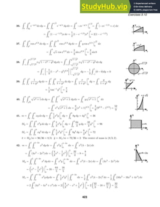

![Exercises 9.10
My =
4
0
√
x
0
(xy + 5x) dy dx =
4
0
1
2
xy2
+ 5xy
√
x
0
dx =
4
0
1
2
x2
+ 5x3/2
dx
=
1
6
x3
+ 2x5/2
4
0
=
224
3
Mx =
4
0
√
x
0
(y2
+ 5y) dy dx =
4
0
1
3
y3
+
5
2
y2
√
x
0
dx =
4
0
1
3
x3/2
+
5
2
x dx
=
2
15
x5/2
+
5
4
x2
4
0
=
364
15
x̄ = My/m =
224/3
92/3
= 56/23; ȳ = Mx/m =
364/15
92/3
= 91/115. The center of mass is (56/23, 91/115).
47. The density is ρ = ky. Since both the region and ρ are symmetric with respect to the
y-axis, x̄ = 0. Using symmetry,
m = 2
1
0
1−x2
0
ky dy dx = 2k
1
0
1
2
y2
1−x2
0
dx = k
1
0
(1 − x2
)2
dx
= k
1
0
(1 − 2x2
+ x4
) dx = k x −
2
3
x3
+
1
5
x5
1
0
= k 1 −
2
3
+
1
5
=
8
15
k
Mx = 2
1
0
1−x2
0
ky2
dy dx = 2k
1
0
1
3
y3
1−x2
0
dx =
2
3
k
1
0
(1 − x2
)3
dx =
2
3
k
1
0
(1 − 3x2
+ 3x4
− x6
) dx
=
2
3
k x − x3
+
3
5
x5
−
1
7
x7
1
0
=
2
3
k 1 − 1 +
3
5
−
1
7
=
32
105
k
ȳ = Mx/m =
32k/105
8k/15
= 4/7. The center of mass is (0, 4/7).
48. The density is ρ = kx.
m =
π
0
sin x
0
kx dy dx =
π
0
kxy
sin x
0
dx =
π
0
kx sin x dx
Integration by parts
= k(sin x − x cos x)
π
0
= kπ
My =
π
0
sin x
0
kx2
dy dx =
π
0
kx2
y
sin x
0
dx =
π
0
kx2
sin x dx Integration by parts
= k(−x2
cos x + 2 cos x + 2x sin x)
π
0
= k[(π2
− 2) − 2] = k(π2
− 4)
Mx =
π
0
sin x
0
kxy dy dx =
π
0
1
2
kxy2
sin x
0
dx =
π
0
1
2
kx sin2
x dx =
π
0
1
4
kx(1 − cos 2x) dx
=
1
4
k
π
0
x dx −
π
0
x cos 2x dx
Integration by parts
=
1
4
k
1
2
x2
π
0
−
1
4
(cos 2x + 2x sin 2x)
π
0
=
1
4
k
1
2
π2
=
1
8
kπ2
x̄ = My/m =
k(π2
− 4)
kπ
= π − 4/π; ȳ = Mx/m =
kπ2
/8
kπ
= π/8. The center of mass is (π − 4/π, π/8).
425](https://image.slidesharecdn.com/advancedengineeringmathematicssolutionsmanual-230807162553-1916df96/85/Advanced-Engineering-Mathematics-Solutions-Manual-pdf-425-320.jpg)
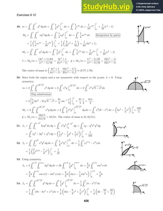
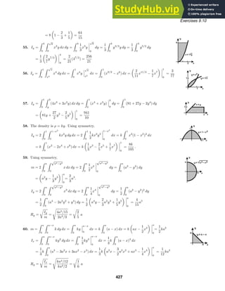
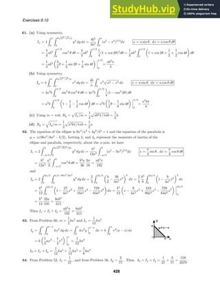
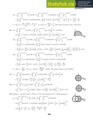
![Exercises 9.11
28.
√
π
−
√
π
√
π−x2
0
sin(x2
+ y2
) dy dx =
π
0
√
π
0
(sin r2
)r dr dθ =
π
0
−
1
2
cos r2
√
π
0
dθ
= −
1
2
π
0
(−1 − 1) dθ = π
29.
1
0
√
4−x2
√
1−x2
x2
x2 + y2
dy dx +
2
1
√
4−x2
0
x2
x2 + y2
dy dx
=
π/2
0
2
1
r2
cos2
θ
r2
r dr dθ =
π/2
0
2
1
r cos2
θ dr dθ
=
π/2
0
1
2
r2
2
1
cos2
θ dθ =
3
2
π/2
0
cos2
θ dθ =
3
2
1
2
θ +
1
4
sin 2θ
π/2
0
=
3π
8
30.
1
0
√
2y−y2
0
(1 − x2
− y2
) dx dy
=
π/4
0
2 sin θ
0
(1 − r2
)r dr dθ +
π/2
π/4
csc θ
0
(1 − r2
)r dr dθ
=
π/4
0
1
2
r2
−
1
4
r4
2 sin θ
0
dθ +
π/2
π/4
1
2
r2
−
1
4
r4
csc θ
0
dθ
=
π/4
0
(2 sin2
θ − 4 sin4
θ) dθ +
π/2
π/4
1
2
csc2
θ −
1
4
csc4
θ dθ
=
θ −
1
2
sin 2θ −
3
2
θ − sin 2θ +
1
8
sin 4θ
+
−
1
2
cot θ −
1
4
− cot θ −
1
3
cot3
θ
π/2
π/4
= −
π
8
+
1
2
+
0 − −
1
4
+
1
12
=
16 − 3π
24
31.
5
−5
√
25−x2
0
(4x + 3y) dy dx =
π
0
5
0
(4r cos θ + 3r sin θ)r dr dθ
=
π
0
5
0
(4r2
cos θ + 3r2
sin θ) dr dθ =
π
0
4
3
r3
cos θ + r3
sin θ
5
0
dθ
=
π
0
500
3
cos θ + 125 sin θ dθ =
500
3
sin θ − 125 cos θ
π
0
= 250
32.
1
0
√
1−y2
0
1
1 + x2 + y2
dx dy =
π/2
0
1
0
1
1 + r
r dr dθ
=
π/2
0
1
0
1 −
1
1 + r
dr dθ =
π/2
0
[r − ln(1 + r)]
1
0
dθ
=
π/2
0
(1 − ln 2)dθ =
π
2
(1 − ln 2)
33. The volume of the cylindrical portion of the tank is Vc = π(4.2)2
19.3 ≈ 1069.56 m3
. We take the equation of
the ellipsoid to be
x2
(4.2)2
+
z2
(5.15)2
= 1 or z = ±
5.15
4.2
(4.2)2 − x2 − y2 .
435](https://image.slidesharecdn.com/advancedengineeringmathematicssolutionsmanual-230807162553-1916df96/85/Advanced-Engineering-Mathematics-Solutions-Manual-pdf-435-320.jpg)
![Exercises 9.11
The volume of the ellipsoid is
Ve = 2
5.15
4.2
R
(4.2)2 − x2 − y2 dx dy =
10.3
4.2
2π
0
4.2
0
[(4.2)2
− r2
]1/2
r dr dθ
=
10.3
4.2
2π
0
−
1
2
2
3
[(4.2)2
− r2
]3/2
4.2
0
dθ =
10.3
4.2
1
3
2π
0
(4.2)3
dθ
=
2π
3
10.3
4.2
(4.2)3
≈ 380.53.
The volume of the tank is approximately 1069.56 + 380.53 = 1450.09 m3
.
34.
R
(x + y) dA =
π/2
0
2
2 sin θ
(r cos θ + r sin θ) r dr dθ =
π/2
0
2
2 sin θ
r2
(cos θ + sin θ) dr dθ
=
π/2
0
1
3
r3
(cos θ + sin θ)
2
2 sin θ
dθ =
8
3
π/2
0
(cos θ + sin θ − sin3
θ cos θ − sin4
θ) dθ
=
8
3
sin θ − cos θ −
1
4
sin4
θ +
1
4
sin3
θ cos θ −
3
8
θ +
3
16
sin 2θ
π/2
0
=
8
3
1 −
1
4
−
3π
16
− (−1)
=
28 − 3π
6
35. I2
=
∞
0
∞
0
e−(x2
+y2
)
dx dy =
π/2
0
∞
0
e−r2
r dr dθ =
π/2
0
lim
t→∞
−
1
2
e−r2
t
0
dθ
=
π/2
0
lim
t→∞
−
1
2
e−t2
+
1
2
dθ =
π/2
0
1
2
dθ =
π
4
; I =
√
π
2
Exercises 9.12
1. The sides of the triangle are C1: y = 0, 0 ≤ x ≤ 1; C2: x = 1, 0 ≤ y ≤ 3; C3: y = 3x,
0 ≤ −x ≤ 1.
ˇC
(x − y) dx + xy dy =
1
0
x dx +
3
0
y dy +
0
1
(x − 3x) dx +
0
1
x(3x) 3 dx
=
1
2
x2
1
0
+
1
2
y2
3
0
+ (−x2
)
1
0
+ (3x2
)
0
1
=
1
2
+
9
2
+ 1 − 3 = 3
R
(y + 1) dA =
1
0
3x
0
(y + 1) dy dx =
1
0
1
2
y2
+ y
3x
0
dx =
1
0
9
2
x2
+ 3x dx
=
3
2
x3
+
3
2
x2
1
0
= 3
2. The sides of the rectangle are C1: y = 0, −1 ≤ x ≤ 1; C2: x = 1, 0 ≤ y ≤ 1; C3: y = 1, 1 ≥ x ≥ −1;
C4: x = −1, 1 ≥ y ≥ 0.
ˇ
C
3x2
y dx + (x2
− 5y) dy =
1
−1
0 dx +
1
0
(1 − 5y) dy =
1
−1
0 dx +
1
0
(1 − 5y) dy
=
−1
1
3x2
dx +
0
1
(1 − 5y) dy = y −
5
2
y2
1
0
+ x3
−1
1
+ y −
5
2
y2
0
1
= −2
R
(2x − 3x2
) dA =
1
0
1
−1
(2x − 3x2
) dx dy =
1
0
(x2
− x3
)
1
−1
dy =
1
0
(−2) dy = −2
436](https://image.slidesharecdn.com/advancedengineeringmathematicssolutionsmanual-230807162553-1916df96/85/Advanced-Engineering-Mathematics-Solutions-Manual-pdf-436-320.jpg)
![Exercises 9.12
3.
ˇC
− y2
dx + x2
dy =
2π
0
(−9 sin2
t)(−3 sin t) dt +
2π
0
9 cos2
t(3 cos t) dt
= 27
2π
0
[(1 − cos2
t) sin t + (1 − sin2
t) cos t] dt
= 27 − cos t +
1
3
cos3
t + sin t −
1
3
sin3
t
2π
0
= 27(0) = 0
R
(2x + 2y) dA = 2
2π
0
3
0
(r cos θ + r sin θ)r dr dθ = 2
2π
0
3
0
r2
(cos θ + sin θ) dr dθ
= 2
2π
0
1
3
r3
(cos θ + sin θ)
3
0
dθ = 18
2π
0
(cos θ + sin θ) dθ
= 18(sin θ − cos θ)
2π
0
= 18(0) = 0
4. The sides of the region are C1: y = 0, 0 ≤ x ≤ 2; C2: y = −x + 2, 2 ≥ x ≥ 1;
C3: y =
√
x , 1 ≥ x ≥ 0.
ˇC
− 2y2
dx + 4xy dy =
2
0
0 dx +
1
2
−2(−x + 2)2
dx +
1
2
4x(−x + 2)(−dx)
+
0
1
−2x dx +
0
1
4x
√
x
1
2
√
x
dx
= 0 +
2
3
+
8
3
+ 1 − 1 =
10
3
R
8y dA =
1
0
2−y
y2
8y dx dy =
1
0
8y(2 − y − y2
) dy = 8y2
−
8
3
y3
− 2y4
1
0
=
10
3
5. P = 2y, Py = 2, Q = 5x, Qx = 5
ˇ
C
2y dx + 5x dy =
R
(5 − 2) dA = 3
R
dA = 3(25π) = 75π
6. P = x + y2
, Py = 2y, Q = 2x2
− y, Qx = 4x
ˇC
(x + y2
) dx + (2x2
− y) dy =
R
(4x − 2y) dA =
2
−2
4
x2
(4x − 2y) dy dx
=
2
−2
(4xy − y2
)
4
x2
dx =
2
−2
(16x − 16 − 4x3
+ x4
) dx
= 8x2
− 16x − x4
+
1
5
x5
2
−2
= −
96
5
7. P = x4
− 2y3
, Py = −6y2
, Q = 2x3
− y4
, Qx = 6x2
. Using polar coordinates,
ˇ
C
(x4
− 2y3
) dx + (2x3
− y4
) dy =
R
(6x2
+ 6y2
) dA =
2π
0
2
0
6r2
r dr dθ
=
2π
0
3
2
r4
2
0
dθ =
2π
0
24 dθ = 48π.
437](https://image.slidesharecdn.com/advancedengineeringmathematicssolutionsmanual-230807162553-1916df96/85/Advanced-Engineering-Mathematics-Solutions-Manual-pdf-437-320.jpg)
![Exercises 9.12
8. P = x − 3y, Py = −3, Q = 4x + y, Qx = 4
ˇ
C
(x − 3y) dx + 4(x + y) dy =
R
(4 + 3) dA = 7(10) = 70
9. P = 2xy, Py = 2x, Q = 3xy2
, Qx = 3y2
ˇ
C
2xy dx + 3xy2
dy =
R
(3y2
− 2x) dA =
2
1
2x
2
(3y2
− 2x) dy dx
=
2
1
(y3
− 2xy)
2x
2
dx =
2
1
(8x3
− 4x2
− 8 + 4x) dx
= 2x4
−
4
3
x3
− 8x + 2x2
2
1
=
40
3
− −
16
3
=
56
3
10. P = e2x
sin 2y, Py = 2e2x
cos 2y, Q = e2x
cos 2y, Qx = 2e2x
cos 2y
ˇ
C
= e2x
sin 2y dx + e2x
cos 2y dy =
R
0 dA = 0
11. P = xy, Py = x, Q = x2
, Qx = 2x. Using polar coordinates,
ˇ
C
xy dx + x2
dy =
R
(2x − x) dA =
π/2
−π/2
1
0
r cos θ r dr dθ
=
π/2
−π/2
1
3
r3
cos θ
1
0
dθ =
π/2
−π/2
1
3
cos θ dθ =
1
3
sin θ
π/2
−π/2
=
2
3
12. P = ex2
, Py = 0, Q = 2 tan−1
x, Qx =
2
1 + x2
ˇC
ex2
dx + 2 tan−1
x dy =
R
2
1 + x2
dA =
0
−1
1
−x
2
1 + x2
dy dx
=
0
−1
2y
1 + x2
1
−x
dx =
0
−1
2
1 + x2
+
2x
1 + x2
dx
= [2 tan−1
x + ln(1 + x2
)]
0
−1
= 0 −
−
π
2
+ ln 2
=
π
2
− ln 2
13. P =
1
3
y3
, Py = y2
, Q = xy + xy2
, Qx = y + y2
ˇC
1
3
y3
dx + (xy + xy2
) dy =
R
y dA =
1/
√
2
0
1−y2
y2
y dx dy
=
1/
√
2
0
(xy)
1−y2
y2
dy =
1/
√
2
0
(y − y3
− y3
) dy
=
1
2
y2
−
1
2
y4
1/
√
2
0
=
1
4
−
1
8
=
1
8
438](https://image.slidesharecdn.com/advancedengineeringmathematicssolutionsmanual-230807162553-1916df96/85/Advanced-Engineering-Mathematics-Solutions-Manual-pdf-438-320.jpg)
 dt +
1
0
[x1 + (x2 − x1)t](y2 − y1) dt
= −(x2 − x1)
y1t +
1
2
(y2 − y1)t2
1
0
+ (y2 − y1)
x1t +
1
2
(x2 − x1)t2
1
0
= −(x2 − x1)
y1 +
1
2
(y2 − y1)
+ (y2 − y1)
x1 +
1
2
(x2 − x1)
= x1y2 − x2y1.
(b) Let Ci be the line segment from (xi, yi) to (xi+1, yi+1) for i = 1, 2, . . . , n − 1, and C2 the line segment
from (xn, yn) to (x1, y1). Then
A =
1
2
ˇ
C
− y dx + x dy Using Problem 18
=
1
2
C1
−y dx + x dy +
C2
−y dx + x dy + · · · +
Cn−1
−y dx + x dy +
Cn
−y dx + x dy
=
1
2
(x1y2 − x2y1) +
1
2
(x2y3 − x3y2) +
1
2
(xn−1yn − xnyn−1) +
1
2
(xny1 − x1yn).
22. From part (b) of Problem 21
A =
1
2
[(−1)(1) − (1)(3)] +
1
2
[(1)(2) − (4)(1)] +
1
2
[(4)(5) − (3)(2)] +
1
2
[(3)(3) − (−1)(5)]
=
1
2
(−4 − 2 + 14 + 14) = 11.
439](https://image.slidesharecdn.com/advancedengineeringmathematicssolutionsmanual-230807162553-1916df96/85/Advanced-Engineering-Mathematics-Solutions-Manual-pdf-439-320.jpg)
![Exercises 9.12
23. P = 4x2
− y3
, Py = −3y2
; Q = x3
+ y2
, Qx = 3x2
.
ˇ
C
(4x2
− y3
) dx + (x3
+ y2
) dy =
R
(3x2
+ 3y2
) dA =
2π
0
2
1
3r2
(r dr dθ) =
2π
0
3
4
r4
2
1
dθ
=
2π
0
45
4
dθ =
45π
2
24. P = cos x2
− y, Py = −1; Q = y3 + 1 , Qx = 0
ˇC
(cos x2
− y) dx + y3 + 1 dy =
R
(0 + 1) dA
R
dA = (6
√
2)2
− π(2)(4) = 72 − 8π
25. We first observe that Py = (y4
− 3x2
y2
)/(x2
= y2
)3
= Qx. Letting C
be the circle x2
+ y2
= 1
4 we have
ˇ
C
−y3
dx + xy2
dy
(x2 + y2)2
=
ˇ
C
−y3
dx + xy2
dy
(x2 + y2)2
x = 1
4 cos t, dx = −1
4 sin t dt, y = 1
4 sin t, dy = 1
4 cos t dt
=
2π
0
− 1
64 sin3
t(−1
4 sin t dt) + 1
4 cos t( 1
16 sin2
t)(1
4 cos t dt)
1/256
=
2π
0
(sin4
t + sin2
t cos2
t) dt =
2π
0
(sin4
t + (sin2
t − sin4
t) dt
=
2π
0
sin2
t dt =
1
2
t −
1
4
sin 2t
2π
0
= π
26. We first observe that Py = [4y2
− (x + 1)2
]/[(x + 1)2
+ 4y2
]2
= Qx. Letting C
be the ellipse (x + 1)2
+ 4y2
= 4
we have
ˇ
C
−y
(x + 1)2 + 4y2
dx +
x + 1
(x + 1)2 + 4y2
dy =
ˇ
C
−y
(x + 1)2 + 4y2
dx +
x + 1
(x + 1)2 + 4y2
dy
x + 1 = 2 cos t, dx = −2 sin t dt, y = sin t, dy = cos t dt
=
2π
0
− sin t
4
(−2 sin t) +
2 cos t
4
cos t
dt =
1
2
2π
0
(sin2
t + cos2
t) dt = π.
27. Writing
R
x2
dA =
R
(Qx − Py)dA we identify Q = 0 and P = −x2
y. Then, with C: x = 3 cos t,
y = 2 sin t, 0 ≤ t ≤ 2π, we have
R
x2
dA =
ˇ
C
P dx + Q dy =
ˇ
C
− x2
y dx = −
2π
0
9 cos2
t(2 sin t)(−3 sin t) dt
=
54
4
2π
0
4 sin2
t cos2
t dt =
27
2
2π
0
sin2
2t dt =
27
4
2π
0
(1 − cos 4t) dt
=
27
4
t −
1
4
sin 4t
2π
0
=
27π
2
.
28. Writing
R
[1 − 2(y − 1)] dA =
R
(Qx − Py) dA we identify Q = x and P = (y − 1)2
. Then, with
440](https://image.slidesharecdn.com/advancedengineeringmathematicssolutionsmanual-230807162553-1916df96/85/Advanced-Engineering-Mathematics-Solutions-Manual-pdf-440-320.jpg)
![Exercises 9.12
C1: x = cos t, y − 1 = sin t, −π/2 ≤ t ≤ π/2, and C2: x = 0, 2 ≥ y ≥ 0,
R
[1 − 2(y − 1)] dA =
C1
P dx + Q dy +
C2
P dx + Q dy =
C1
(y − 1)2
dx + x dy +
C2
0 dy
=
π/2
−π/2
[sin2
t(− sin t) + cos t cos t] dt =
π/2
−π/2
[cos2
t − (1 − cos2
t) sin t] dt
=
π/2
−π/2
1
2
(1 + cos 2t) − sin t + cos2
t sin t
dt
=
1
2
t +
1
4
sin 2t + cos t −
1
3
cos3
t
π/2
−π/2
=
π
4
−
−
π
4
=
π
2
.
29. P = x − y, Py = −1, Q = x + y, Qx = 1; W =
ˇ
C
F · d r =
R
2 dA = 2 × area = 2
3π
4
=
3
2
π
30. P = −xy2
, Py = −2xy, Q = x2
y, Qx = 2xy. Using polar coordinates,
W =
ˇ
C
F · dr =
R
4xy dA =
π/2
0
2
1
4(r cos θ)(r sin θ)r dr dθ =
π/2
0
(r4
cos θ sin θ)
2
1
dθ
= 15
π/2
0
sin θ cos θ dθ =
15
2
sin2
θ
π/2
0
=
15
2
.
31. Since
B
A
P dx + Q dy is independent of path, Py = Qx by Theorem 9.9. Then, by Green’s Theorem
ˇ
C
P dx + Q dy =
R
(Qx − Py) dA =
R
0 dA = 0.
32. Let P = 0 and Q = x2
. Then Qx − Py = 2x and
1
2A
ˇC
x2
dy =
1
2A
R
2x dA =
R
x dA
A
= x̄.
Let P = y2
and Q = 0. Then Qx − Py = −2y and
−
1
2A
ˇC
y2
dx = −
1
2A
R
−2y dA =
R
y dA
A
= ȳ.
33. Using Green’s Theorem,
W =
ˇ
C
F · dr =
ˇ
C
− y dx + x dy =
R
2 dA = 2
2π
0
1+cos θ
0
r dr dθ
= 2
2π
0
1
2
r2
1+cos θ
0
dθ =
2π
0
(1 + 2 cos θ + cos2
θ) dθ
= θ + 2 sin θ +
1
2
θ +
1
4
sin 2θ
2π
0
= 3π.
441](https://image.slidesharecdn.com/advancedengineeringmathematicssolutionsmanual-230807162553-1916df96/85/Advanced-Engineering-Mathematics-Solutions-Manual-pdf-441-320.jpg)
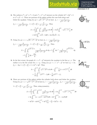
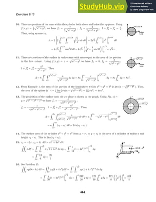
![Exercises 9.13
21. zx = −x, zy = −y; dS = 1 + x2 + y2 dA
S
xy dS =
1
0
1
0
xy 1 + x2 + y2 dx dy =
1
0
1
3
y(1 + x2
+ y2
)3/2
1
0
dy
=
1
0
1
3
y(2 + y2
)3/2
−
1
3
y(1 + y2
)3/2
dy
=
1
15
(2 + y2
)5/2
−
1
15
(1 + y2
)5/2
1
0
=
1
15
(35/2
− 27/2
+ 1)
22. z =
1
2
+
1
2
x2
+
1
2
y2
, zx = x, zy = y; dS = 1 + x2 + y2 dA.
Using polar coordinates,
S
2z dS =
R
(1 + x2
+ y2
) 1 + x2 + y2 dA
=
π/2
π/3
1
0
(1 + r2
) 1 + r2 r dr dθ
=
π/2
π/3
1
0
(1 + r2
)3/2
r dr dθ =
π/2
π/3
1
5
(1 + r2
)5/2
1
0
dθ =
1
5
π/2
π/3
(25/2
− 1) dθ
=
4
√
2 − 1
5
π
2
−
π
3
=
(4
√
2 − 1)π
30
.
23. yx = 2x, yz = 0; dS =
√
1 + 4x2 dA
S
24
√
y z dS =
3
0
2
0
24xz 1 + 4x2 dx dz =
3
0
2z(1 + 4x2
)3/2
2
0
dz
= 2(173/2
− 1)
3
0
z dz = 2(173/2
− 1)
1
2
z2
3
0
= 9(173/2
− 1)
24. xy = −2y, xz = −2z; dS = 1 + 4y2 + 4z2 dA.
Using polar coordinates,
S
(1 + 4y2
+ 4z2
)1/2
dS =
π/2
0
2
1
(1 + 4r2
)r dr dθ
=
π/2
0
1
16
(1 + 4r2
)2
2
1
dθ =
1
16
π/2
0
12 dθ =
3π
8
.
25. Write the equation of the surface as y =
1
2
(6 − x − 3z).
yx = −
1
2
, yz = −
3
2
; dS = 1 + 1/4 + 9/4 =
√
14
2
.
S
(3z2
+ 4yz) dS =
2
0
6−3z
0
3z2
+ 4z
1
2
(6 − x − 3z)
√
14
2
dx dz
=
√
14
2
2
0
[3z2
x − z(6 − x − 3z)2
]
6−3z
0
dz
=
√
14
2
2
0
[3z2
(6 − 3z) − 0] − [0 − z(6 − 3z)2
]
dz
=
√
14
2
2
0
(36z − 18z2
) dz =
√
14
2
(18z2
− 6z3
)
2
0
=
√
14
2
(72 − 48) = 12
√
14
446](https://image.slidesharecdn.com/advancedengineeringmathematicssolutionsmanual-230807162553-1916df96/85/Advanced-Engineering-Mathematics-Solutions-Manual-pdf-446-320.jpg)
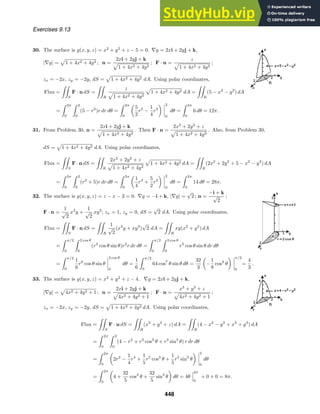
![Exercises 9.13
34. The surface is g(x, y, z) = x+y +z −6. ∇g = i+j+k, |∇g| =
√
3 ; n = (i+j+k)/
√
3 ;
F · n = (ey
+ ex
+ 18y)/
√
3 ; zx = −1, zy = −1, dS =
√
1 + 1 + 1 dA =
√
3 dA.
Flux =
S
F · n dS =
r
(ey
+ ex
+ 18y) dA =
6
0
6−x
0
(ey
+ ex
+ 18y) dy dx
=
6
0
(ey
+ yex
+ 9y2
)
6−x
0
dx =
6
0
[e6−x
+ (6 − x)ex
+ 9(6 − x)2
− 1] dx
= [−e6−x
+ 6ex
− xex
+ ex
− 3(6 − x)3
− x]
6
0
= (−1 + 6e6
− 6e6
+ e6
− 6) − (−e6
+ 6 + 1 − 648) = 2e6
+ 634 ≈ 1440.86
35. For S1: g(x, y, z) = x2
+ y2
− z, ∇g = 2xi + 2yj − k, |∇g| = 4x2 + 4y2 + 1 ; n1 =
2xi + 2yj − k
4x2 + 4y2 + 1
;
F · n1 =
2xy2
+ 2x2
y − 5z
4x2 + 4y2 + 1
; zx = 2x, zy = 2y, dS1 = 1 + 4x2 + 4y2 dA. For S2: g(x, y, z) = z − 1,
∇g = k, |∇g| = 1; n2 = k; F·n2 = 5z; zx = 0, zy = 0, dS2 = dA. Using polar coordinates and R: x2
+y2
≤ 1
we have
Flux =
S1
F · n1 dS1 +
S2
F · n2 dS2 =
R
(2xy2
+ 2x2
y − 5z) dA +
R
5z dA
=
R
[2xy2
+ 2x2
y − 5(x2
+ y2
) + 5(1)] dA
=
2π
0
1
0
(2r3
cos θ sin2
θ + 2r3
cos2
θ sin θ − 5r2
+ 5)r dr dθ
=
2π
0
2
5
r5
cos θ sin2
θ +
2
5
r5
cos2
θ sin θ −
5
4
r4
+
5
2
r2
1
0
dθ
=
2π
0
2
5
(cos θ sin2
θ + cos2
θ sin θ) +
5
4
dθ =
2
5
1
3
sin3
θ −
1
3
cos3
θ
2π
0
+
5
4
θ
2π
0
=
2
5
−
1
3
− −
1
3
+
5
2
π =
5
2
π.
36. For S1: g(x, y, z) = x2
+ y2
+ z − 4, ∇g = 2xi + 2yj + k, |∇g| = 4x2 + 4y2 + 1 ;
n1 =
2xi + 2yj + k
4x2 + 4y2 + 1
; F · n1 = 6z2
/ 4x2 + 4y2 + 1 ; zx = −2x, zy = −2y,
dS1 = 1 + 4x2 + 4y2 dA. For S2: g(x, y, z) = x2
+ y2
− z, ∇g = 2xi + 2yj − k,
|∇g| = 4x2 + 4y2 + 1 ; n2 =
2xi + 2yj − k
4x2 + y2 + 1
; F · n2 = −6z2
/ 4x2 + 4y2 + 1 ; zx = 2x, zy = 2y,
dS2 = 1 + 4x2 + 4y2 dA. Using polar coordinates and R: x2
+ y2
≤ 2 we have
Flux =
S1
F · n1 dS1 +
S1
F · n2 dS2 =
R
6z2
dA +
−6z2
dA
=
R
[6(4 − x2
− y2
)2
− 6(x2
+ y2
)2
] dA = 6
2π
0
√
2
0
[(4 − r2
)2
− r4
] r dr dθ
= 6
2π
0
−
1
6
(4 − r2
)3
−
1
6
r6
√
2
0
dθ = −
2π
0
[(23
− 43
) + (
√
2 )6
] dθ =
2π
0
48 dθ = 96π.
449](https://image.slidesharecdn.com/advancedengineeringmathematicssolutionsmanual-230807162553-1916df96/85/Advanced-Engineering-Mathematics-Solutions-Manual-pdf-449-320.jpg)
![Exercises 9.14
z̄ =
1
3
√
14
S
z dS =
1
3
√
14
3
0
2−2x/3
0
(6 − 2x − 3y)
√
14 dy dx
=
1
3
3
0
6y − 2xy −
3
2
y2
2−2x/3
0
dx =
1
3
3
0
6 − 4x +
2
3
x2
dx =
1
3
6x − 2x2
+
2
9
x3
3
0
= 2
The centroid is (1, 2/3, 2).
42. The area of the hemisphere is A(s) = 2πa2
. By symmetry, x̄ = ȳ = 0.
zx = −
x
a2 − x2 − y2
, zy = −
y
a2 − x2 − y2
;
dS =
1 +
x2
a2 − x2 − y2
+
y2
a2 − x2 − y2
dA =
a
a2 − x2 − y2
dA
Using polar coordinates,
z =
S
z dS
2πa2
=
1
2πa2
R
a2 − x2 − y2
a
a2 − x2 − y2
dA =
1
2πa
2π
0
a
0
r dr dθ
=
1
2πa
2π
0
1
2
r2
a
0
dθ =
1
2πa
2π
0
1
2
s2
dθ =
a
2
.
The centroid is (0, 0, a/2).
43. The surface is g(x, y, z) = z − f(x, y) = 0. ∇g = −fxi − fyj + k, |∇g| = f2
x + f2
y + 1 ;
n =
−fxi − fyj + k
1 + f2
x + f2
y
; F · n =
−Pfx − Qfy + R
1 + f2
x + f2
y
; dS = 1 + f2
x + f2
y dA
S
F · n dS =
R
−Pfx − Qfy + R
1 + f2
x + f2
y
1 + f2
x + f2
y dA =
R
(−Pfx − Qfy + R) dA
Exercises 9.14
1. Surface Integral: curl F = −10k. Letting g(x, y, z) = z − 1, we have ∇g = k and n = k. Then
S
(curl F) · n dS =
S
(−10) dS = −10 × (area of S) = −10(4π) = −40π.
Line Integral: Parameterize the curve C by x = 2 cos t, y = 2 sin t, z = 1, for 0 ≤ t ≤ 2π. Then
ˇC
F · dr =
ˇC
5y dx − 5x dy + 3 dz =
2π
0
[10 sin t(−2 sin t) − 10 cos t(2 cos t)] dt
=
2π
0
(−20 sin2
t − 20 cos2
t) dt =
2π
0
−20 dt = −40π.
2. Surface Integral: curl F = 4i − 2j − 3k. Letting g(x, y, z) = x2
+ y2
+ z − 16,
∇g = 2xi + 2yj + k, and n = (2xi + 2yj + k)/ 4x2 + 4y2 + 1 . Thus,
S
(curl F) · n dS =
S
8x − 4y − 3
4x2 + 4y2 + 1
dS.
Letting the surface be z = 16 − x2
− y2
, we have zx = −2x, zy = −2y, and
dS = 1 + 4x2 + 4y2 dA. Then, using polar coordinates,
451](https://image.slidesharecdn.com/advancedengineeringmathematicssolutionsmanual-230807162553-1916df96/85/Advanced-Engineering-Mathematics-Solutions-Manual-pdf-451-320.jpg)
![Exercises 9.14
S
(curl F) · n dS =
R
(8x − 4y − 3) dA =
2π
0
4
0
(8r cos θ − 4r sin θ − 3) r dr dθ
=
2π
0
8
3
r3
cos θ −
4
3
r3
sin θ −
3
2
r2
4
0
dθ =
2π
0
512
3
cos θ −
256
3
sin θ − 24 dθ
=
512
3
sin θ +
256
3
cos θ − 24θ
2π
0
= −48π.
Line Integral: Parameterize the curve C by x = 4 cos t, y = 4 sin t, z = 0, for 0 ≤ t ≤ 2π. Then,
ˇC
F · dr =
ˇC
2z dx − 3x dy + 4y dz =
2π
0
[−12 cos t(4 cos t)] dt
=
2π
0
−48 cos2
t dt = (−24t − 12 sin 2t)
2π
0
= −48π.
3. Surface Integral: curl F = i + j + k. Letting g(x, y, z) = 2x + y + 2z − 6, we have
∇g = 2i+j+2k and n = (2i+j+2k)/3. Then
S
(curl F)·n dS =
S
5
3
dS. Letting
the surface be z = 3 − 1
2 y − x we have zx = −1, zy = −1
2 , and
dS = 1 + (−1)2 + (−1
2 )2 dA = 3
2 dA. Then
S
(curl F) · n dS =
R
5
3
3
2
dA =
5
2
× (area of R) =
5
2
(9) =
45
2
.
Line Integral: C1: z = 3−x, 0 ≤ x ≤ 3, y = 0; C2: y = 6−2x, 3 ≥ x ≥ 0, z = 0; C3: z = 3−y/2, 6 ≥ y ≥ 0,
x = 0.
ˇ
C
z dx + x dy + y dz =
C1
z dx +
C2
x dy +
C3
y dz
=
3
0
(3 − x) dx +
0
3
x(−2 dx) +
0
6
y(−dy/2)
= 3x −
1
2
x2
3
0
−x2
0
3
−
1
4
y2
0
6
=
9
2
− (0 − 9) −
1
4
(0 − 36) =
45
2
4. Surface Integral: curl F = 0 and
S
(curl F) · n dS = 0.
Line Integral: the curve is x = cos t, y = sin t, z = 0, 0 ≤ t ≤ 2π.
ˇC
x dx + y dy + z dz =
2π
0
[cos t(− sin t) + sin t(cos t)]dt = 0.
5. curl F = 2i + j. A unit vector normal to the plane is n = (i + j + k)/
√
3 . Taking the
equation of the plane to be z = 1 − x − y, we have zx = zy = −1. Thus,
dS =
√
1 + 1 + 1 dA =
√
3 dA and
ˇ
C
F · dr =
S
(curl F) · n dS =
S
√
3 dS =
√
3
R
√
3 dA
= 3 × (area of R) = 3(1/2) = 3/2.
6. curl F = −2xzi + z2
k. A unit vector normal to the plane is n = (j + k)/
√
2 . From z = 1 − y, we have zx = 0
and zy = −1. Thus, dS =
√
1 + 1 dA =
√
2 dA and
452](https://image.slidesharecdn.com/advancedengineeringmathematicssolutionsmanual-230807162553-1916df96/85/Advanced-Engineering-Mathematics-Solutions-Manual-pdf-452-320.jpg)
![Exercises 9.14
ˇ
C
F · dr =
S
(curl F) · n dS =
R
1
√
2
z2
√
2 dA =
R
(1 − y)2
dA
=
2
0
1
0
(1 − y)2
dy dx =
2
0
−
1
3
(1 − y)3
1
0
dx =
2
0
1
3
dx =
2
3
.
7. curl F = −2yi − zj − xk. A unit vector normal to the plane is n = (j + k)/
√
2 . From z = 1 − y we have zx = 0
and zy = −1. Then dS =
√
1 + 1 dA =
√
2 dA and
ˇC
F · dr =
S
(curl F) · n dS =
R
−
1
√
2
(z + x)
√
2 dA =
R
(y − x − 1) dA
=
2
0
1
0
(y − x − 1) dy dx =
2
0
1
2
y2
− xy − y
1
0
dx =
2
0
−x −
1
2
dx
= −
1
2
x2
−
1
2
x
2
0
= −3.
8. curl F = 2i + 2j + 3k. Letting g(x, y, z) = x + 2y + z − 4, we have ∇g = i + 2j + k
and n = (i + 2j + k)/
√
6 . From z = 4 − x − 2y we have zx = −1 and zy = −2. Then
dS =
√
6 dA and
ˇ
C
F · dr =
S
(curl F) · n dS =
R
1
√
6
(9)
√
6 dA =
R
9 dA = 9(4) = 36.
9. curl F = (−3x2
− 3y2
)k. A unit vector normal to the plane is n = (i + j + k)/
√
3 . From
z = 1 − x − y, we have zx = zy = −1 and dS =
√
3 dA. Then, using polar coordinates,
ˇ
C
F · dr =
S
(curl F) · n dS =
R
(−
√
3 x2
−
√
3 y2
)
√
3 dA
= 3
R
(−x2
− y2
) dA = 3
2π
0
1
0
(−r2
)r dr dθ
= 3
2π
0
−
1
4
r4
1
0
dθ = 3
2π
0
−
1
4
dθ = −
3π
2
.
10. curl F = 2xyzi − y2
zj + (1 − x2
)k. A unit vector normal to the surface is n =
2yj + k
4y2 + 1
. From z = 9 − y2
we have zx = 0, zy = −2y and dS = 1 + 4y2 dA. Then
ˇ
C
F · dr =
S
(curl F) · n dS =
R
(−2y3
z + 1 − x2
) dA =
3
0
y/2
0
[−2y3
(9 − y2
) + 1 − x2
] dx dy
=
3
0
−18y3
x + 2y5
x + x −
1
3
x3
y/2
0
dy =
3
0
−9y4
+ y6
+
1
2
y −
1
24
y3
dy
= −
9
5
y5
+
1
7
y7
+
1
4
y2
−
1
96
y4
3
0
≈ 123.57.
11. curl F = 3x2
y2
k. A unit vector normal to the surface is
n =
8xi + 2yj + 2zk
64x2 + 4y2 + 4z2
=
4xi + yj + zk
16x2 + y2 + z2
.
453](https://image.slidesharecdn.com/advancedengineeringmathematicssolutionsmanual-230807162553-1916df96/85/Advanced-Engineering-Mathematics-Solutions-Manual-pdf-453-320.jpg)
![Exercises 9.14
From zx = −
4x
4 − 4x2 − y2
, zy = −
y
4 − 4x2 − y2
we obtain dS = 2
1 + 3x2
4 − 4x2 − y2
dA. Then
ˇ
C
F · dr =
S
(curl F) · n dS =
R
3x2
y2
z
16x2 + y2 + z2
2
1 + 3x2
4 − 4x2 − y2
dA
=
R
3x2
y2
dA Using symmetry
= 12
1
0
2
√
1−x2
0
x2
y2
dy dx = 12
1
0
1
3
x2
y3
2
√
1−x2
0
dx
= 32
1
0
x2
(1 − x2
)3/2
dx x = sin t, dx = cos t dt
= 32
π/2
0
sin2
t cos4
t dt = π.
12. curl F = i + j + k. Taking the surface S bounded by C to be the portion of the plane
x + y + z = 0 inside C, we have n = (i + j + k)/
√
3 and dS =
√
3 dA.
ˇ
C
F · dr =
S
(curl F) · n dS =
S
√
3 dS =
√
3
R
√
3 dA = 3 × (area of R)
The region R is obtained by eliminating z from the equations of the plane and the sphere.
This gives x2
+ xy + y2
= 1
2 . Rotating axes, we see that R is enclosed by the ellipse
X2
/(1/3) + Y 2
/1 = 1 in a rotated coordinate system. Thus,
ˇ
C
F · dr = 3 × (area of R) = 3 π
1
√
3
1 =
√
3 π.
13. Parameterize C by x = 4 cos t, y = 2 sin t, z = 4, for 0 ≤ t ≤ 2π. Then
S
(curl F) · n dS =
ˇ
C
F · dr =
ˇ
C
6yz dx + 5x dy + yzex2
dz
=
2π
0
[6(2 sin t)(4)(−4 sin t) + 5(4 cos t)(2 cos t) + 0] dt
= 8
2π
0
(−24 sin2
t + 5 cos2
t) dt = 8
2π
0
(5 − 29 sin2
t) dt = −152π.
14. Parameterize C by x = 5 cos t, y = 5 sin t, z = 4, for 0 ≤ t ≤ 2π. Then,
S
(curl F) · n dS =
ˇ
C
F · r =
ˇ
C
y dx + (y − x) dy + z2
dz
=
2π
0
[(5 sin t)(−5 sin t) + (5 sin t − 5 cos t)(5 cos t)] dt
=
2π
0
(25 sin t cos t − 25) dt =
25
2
sin2
t − 25t
2π
0
= −50π.
454](https://image.slidesharecdn.com/advancedengineeringmathematicssolutionsmanual-230807162553-1916df96/85/Advanced-Engineering-Mathematics-Solutions-Manual-pdf-454-320.jpg)
![Exercises 9.14
15. Parameterize C by C1: x = 0, z = 0, 2 ≥ y ≥ 0; C2: z = x, y = 0, 0 ≤ x ≤ 2;
C3: x = 2, z = 2, 0 ≤ y ≤ 2; C4: z = x, y = 2, 2 ≥ x ≥ 0. Then
S
(curl F) · n dS =
ˇ
C
F · r =
ˇ
C
3x2
dx + 8x3
y dy + 3x2
y dz
=
C1
0 dx + 0 dy + 0 dz +
C2
3x2
dx +
C3
64 dy +
C4
3x2
dx + 6x2
dx
=
2
0
3x2
dx +
2
0
64 dy +
0
2
9x2
dx = x3
2
0
+ 64y
2
0
+ 3x3
0
2
= 112.
16. Parameterize C by x = cos t, y = sin t, z = sin t, 0 ≤ t ≤ 2π. Then
S
(curl F) · n dS =
ˇC
F · r =
ˇC
2xy2
z dx + 2x2
yz dy + (x2
y2
− 6x) dz
=
2π
0
[2 cos t sin2
t sin t(− sin t) + 2 cos2
t sin t sin t cos t
+ (cos2
t sin2
t − 6 cos t) cos t] dt
=
2π
0
(−2 cos t sin4
t + 3 cos3
t sin2
t − 6 cos2
t) dt = −6π.
17. We take the surface to be z = 0. Then n = k and dS = dA. Since curl F =
1
1 + y2
i + 2zex2
j + y2
k,
ˇ
C
z2
ex2
dx + xy dy + tan−1
y dz =
S
(curl F) · n dS =
S
y2
dS =
R
y2
dA
=
2π
0
3
0
r2
sin2
θ r dr dθ =
2π
0
1
4
r4
sin2
θ
3
0
dθ
=
81
4
2π
0
sin2
θ dθ =
81π
4
.
18. (a) curl F = xzi − yzj. A unit vector normal to the surface is n =
2xi + 2yj + k
4x2 + 4y2 + 1
and
dS = 1 + 4x2 + 4y2 dA. Then, using x = cos t, y = sin t, 0 ≤ t ≤ 2π, we have
S
(curl F) · n dS =
R
(2x2
z − 2y2
z) dA =
R
(2x2
− 2y2
)(1 − x2
− y2
) dA
=
R
(2x2
− 2y2
− 2x4
+ 2y4
) dA
=
2π
0
1
0
(2r2
cos2
θ − 2r2
sin2
θ − 2r4
cos4
θ + 2r4
cos4
θ) r dr dθ
= 2
2π
0
1
0
[r3
cos 2θ − r5
(cos2
θ − sin2
θ)(cos2
θ + sin2
θ)] dr dθ
= 2
2π
0
1
0
(r3
cos 2θ − r5
cos 2θ) dr dθ = 2
2π
0
cos 2θ
1
4
r4
−
1
6
r6
1
0
dθ
=
1
6
2π
0
cos 2θ dθ = 0.
(b) We take the surface to be z = 0. Then n = k, curl F · n = curl F · k = 0 and
S
(curl F) · n dS = 0.
455](https://image.slidesharecdn.com/advancedengineeringmathematicssolutionsmanual-230807162553-1916df96/85/Advanced-Engineering-Mathematics-Solutions-Manual-pdf-455-320.jpg)
![Exercises 9.14
(c) By Stoke’s Theorem, using z = 0, we have
S
(curl F) · n dS =
ˇ
C
F · dr =
ˇ
C
xyz dz =
ˇ
C
xy(0) dz = 0.
Exercises 9.15
1.
4
2
2
−2
1
−1
(x + y + z)dx dy dz =
4
2
2
−2
1
2
x2
+ xy + xz
1
−1
dy dz
=
4
2
2
−2
(2y + 2z) dy dz =
4
2
(y2
+ 2yz)
2
−2
dz =
4
2
8z dz = 4z2
4
2
= 48
2.
3
1
x
1
xy
2
24xy dz dy dx =
3
1
x
1
24xyz
xy
2
dy dx =
3
1
x
1
(24x2
y2
− 48xy)dy dx
=
3
1
(8x2
y3
− 24xy2
)
x
1
dx =
3
1
(8x5
− 24x3
− 8x2
+ 24x) dx
=
4
3
x6
− 6x4
−
8
3
x3
+ 12x2
3
1
= 522 −
14
3
=
1552
3
3.
6
0
6−x
0
6−x−z
0
dy dz dx =
6
0
6−x
0
(6 − x − z)dz dx =
6
0
6z − xz −
1
2
z2
6−x
0
dx
=
6
0
6(6 − x) − x(6 − x) −
1
2
(6 − x)2
dx =
6
0
18 − 6x +
1
2
x2
dx
= 18x − 3x2
+
1
6
x3
6
0
= 36
4.
1
0
1−x
0
√
y
0
4x2
z3
dz dy dx =
1
0
1−x
0
x2
z4
√
y
0
dy dx =
1
0
1−x
0
x2
y2
dy dx
=
1
0
1
3
x2
y3
1−x
0
dx =
1
3
1
0
x2
(1 − x)3
dx =
1
3
1
0
(x2
− 3x3
+ 3x4
− x5
)dx
=
1
3
1
3
x3
−
3
4
x4
+
3
5
x5
−
1
6
x6
1
0
=
1
180
5.
π/2
0
y2
0
y
0
cos
x
y
dz dx dy =
π/2
0
y2
0
y cos
x
y
dx dy =
π/2
0
y2
sin
x
y
y2
0
dy
=
π/2
0
y2
sin y dy Integration by parts
= (−y2
cos y + 2 cos y + 2y sin y)
π/2
0
= π − 2
6.
√
2
0
2
√
y
ex2
0
x dz dx dy =
√
2
0
2
√
y
xex2
dx dy =
√
2
0
1
2
ex2
2
√
y
dy =
1
2
√
2
0
(e4
− ey
)dy
=
1
2
(ye4
− ey
)
√
2
0
=
1
2
[(e4
√
2 − e
√
2
) − (−1)] =
1
2
(1 + e4
√
2 − e
√
2
)
456](https://image.slidesharecdn.com/advancedengineeringmathematicssolutionsmanual-230807162553-1916df96/85/Advanced-Engineering-Mathematics-Solutions-Manual-pdf-456-320.jpg)

![Exercises 9.15
Mxy =
1
0
2−z
z2
3
0
z dy dx dz =
1
0
2−z
z2
yz
3
0
dx dz =
1
0
2−z
z2
3z dx dz
= 3
1
0
xz
2−z
z2
dz = 3
1
0
(2z − z2
− z3
) dz = 3 z2
−
1
3
z3
−
1
4
z4
1
0
=
5
4
Mxz =
1
0
2−z
z2
3
0
y dy dx dz =
1
0
2−z
z2
1
2
y2
3
0
dx dz =
9
2
1
0
2−z
z2
dx dz
=
9
2
1
0
(2 − z − z2
) dz =
9
2
2z −
1
2
z2
−
1
3
z3
1
0
=
21
4
Myz =
1
0
2−z
z2
3
0
x dy dx dz =
1
0
2−z
z2
xy
3
0
dx dz =
1
0
2−x
z2
3x dx dz
= 3
1
0
1
2
x2
2−z
z2
dz =
3
2
1
0
(4 − 4z + z2
− z4
) dz =
3
2
4z − 2z2
+
1
3
z3
−
1
5
z5
1
0
=
16
5
x̄ = Myz/m =
16/5
7/2
= 32/35, ȳ = Mxz/m =
21/4
7/2
= 3/2, z̄ = Mxy/m =
5/4
7/2
= 5/14.
The centroid is (32/35, 3/2, 5/14).
27. The density is ρ(x, y, z) = ky. Since both the region and the density function are symmetric
with respect to the xy-and yz-planes, x̄ = z̄ = 0. Using symmetry,
m = 4
3
0
2
0
√
4−x2
0
ky dz dx dy = 4k
3
0
2
0
yz
√
4−x2
0
dx dy = 4k
3
0
2
0
y 4 − x2 dx dy
= 4k
3
0
y
x
2
4 − x2 + 2 sin−1 x
2
2
0
dy = 4k
3
0
πy dy = 4πk
1
2
y2
3
0
= 18πk
Mxz = 4
3
0
2
0
√
4−x2
0
ky2
dz dx dy = 4k
3
0
2
0
y2
z
√
4−x2
0
dx dy = 4k
3
0
2
0
y2
4 − x2 dx dy
= 4k
3
0
y2
x
2
4 − x2 + 2 sin−1 x
2
2
0
dy = 4k
3
0
πy2
dy = 4πk
1
3
y3
3
0
= 36πk.
ȳ = Mxz/m =
36πk
18πk
= 2. The center of mass is (0, 2, 0).
28. The density is ρ(x, y, z) = kz.
m =
1
0
x
x2
y+2
0
kz dz dy dx = k
1
0
x
x2
1
2
z2
y+2
0
dy dx
=
1
2
k
1
0
x
x2
(y + 2)2
dy dx =
1
2
k
1
0
1
3
(y + 2)3
x
x2
dx
=
1
6
k
1
0
[(x + 2)3
− (x2
+ 2)3
] dx =
1
6
k
1
0
[(x + 2)3
− (x6
+ 6x4
+ 12x2
+ 8)]dx
=
1
6
k
1
4
(x + 2)4
−
1
7
x7
−
6
5
x5
− 4x3
− 8x
1
0
=
407
840
k
460](https://image.slidesharecdn.com/advancedengineeringmathematicssolutionsmanual-230807162553-1916df96/85/Advanced-Engineering-Mathematics-Solutions-Manual-pdf-460-320.jpg)
![Exercises 9.15
Mxy =
1
0
x
x2
y+2
0
kz2
dz dy dx = k
1
0
x
x2
1
3
z3
y+2
0
dy dx =
1
3
k
1
0
x
x2
(y + 2)3
dy dx
=
1
3
k
1
0
1
4
(y + 2)4
x
x2
dx =
1
12
k
1
0
[(x + 2)4
− (x2
+ 2)4
] dx
=
1
12
k
1
0
[(x + 2)4
− (x8
+ 8x6
+ 24x4
+ 32x2
+ 16)] dx
=
1
12
k
1
5
(x + 2)5
−
1
9
x9
−
8
7
x7
−
24
5
−
32
3
x3
− 16x
1
0
=
1493
1890
k
Mxz =
1
0
x
x2
y+2
0
kyz dz dy dx = k
1
0
x
x2
1
2
yz2
y+2
0
dy dx =
1
2
k
1
0
x
x2
y(y + 2)2
dy dx
=
1
2
k
1
0
x
x2
(y3
+ 4y2
+ 4y) dy dx =
1
2
k
1
0
1
4
y4
+
4
3
y3
+ 2y2
x
x2
dx
=
1
2
k
1
0
−
1
4
x8
−
4
3
x6
− 74x4
+
4
3
x3
+ 2x2
dx
=
1
2
k −
1
36
x9
−
4
21
x7
−
7
20
x5
+
1
3
x4
+
2
3
x3
1
0
=
68
315
k
Myz =
1
0
x
x2
y+2
0
kxz dz dy dx = k
1
0
x
x2
1
2
xz2
y+2
0
dy dx =
1
2
k
1
0
x
x2
x(y + 2)2
dy dx
=
1
2
k
1
0
1
3
x(y + 2)3
x
x2
dx =
1
6
k
1
0
[x(x + 2)3
− x(x2
+ 2)3
] dx
=
1
6
k
1
0
[x4
+ 6x3
+ 12x2
+ 8x − x(x2
+ 2)3
] dx
=
1
6
k
1
5
x5
+
3
2
x4
+ 4x3
+ 4x2
−
1
8
(x2
+ 2)4
1
0
=
21
80
k
x̄ = Myz/m =
21k/80
407k/840
= 441/814, ȳ = Mxz/m =
68k/315
407k/840
= 544/1221,
z̄ = Mxy/m =
1493k/1890
407k/840
= 5972/3663. The center of mass is (441/814, 544/1221, 5972/3663).
29. m =
1
−1
√
1−x2
−
√
1−x2
8−y
2+2y
(x + y + 4) dz dy dx
30. Both the region and the density function are symmetric with respect to the xz- and
yz-planes. Thus, m = 4
2
−1
√
1+z2
0
√
1+z2−y2
0
z2
dx dy dz.
461](https://image.slidesharecdn.com/advancedengineeringmathematicssolutionsmanual-230807162553-1916df96/85/Advanced-Engineering-Mathematics-Solutions-Manual-pdf-461-320.jpg)


![Exercises 9.16
z̄ = Mxy/m =
2kπ/15
kπ/4
= 8/15. The center of mass is (0, 0, 8/15).
81. We are given density = k/ρ.
m =
2π
0
cos−1
4/5
0
5
4 sec φ
k
ρ
ρ2
sin φ dρ dφ dθ = k
2π
0
cos−1
4/5
0
1
2
ρ2
sin φ
5
4 sec φ
dφ dθ
=
1
2
k
2π
0
cos−1
4/5
0
(25 sin φ − 16 tan φ sec φ) dφ dθ
=
1
2
k
2π
0
(−25 cos φ − 16 sec φ)
cos−1
4/5
0
dθ =
1
2
k
2π
0
[−25(4/5) − 16(5/4) − (−25 − 16)] dθ
=
1
2
k
2π
0
dθ = kπ
82. We are given density = kρ.
Iz =
2π
0
π
0
a
0
(x2
+ y2
)(kρ)ρ2
sin φ dρ dφ dθ
= k
2π
0
π
0
a
0
(ρ2
sin2
φ cos2
θ + ρ2
sin2
φ sin2
θ)ρ3
sin φ dρ dφ dθ
= k
2π
0
π
0
a
0
ρ5
sin3
φ dρ dφ dθ = k
2π
0
π
0
1
6
ρ6
sin3
φ
a
0
dφ dθ =
1
6
ka6
2π
0
π
0
sin3
φ dφ dθ
=
1
6
ka3
2π
0
π
0
(1 − cos2
φ) sin φ dφ dθ =
1
6
ka3
2π
0
− cos φ +
1
3
cos3
φ
π
0
dθ =
1
6
ka3
2π
0
4
3
dθ =
4π
9
ka6
Exercises 9.16
1. div F = y + z + x
The Triple Integral:
D
div F dV =
1
0
1
0
1
0
(x + y + z) dx dy dz
=
1
0
1
0
1
2
x2
+ xy + xz
1
0
dy dz
=
1
0
1
0
1
2
+ y + z dy dz =
1
0
1
2
y +
1
2
y2
+ yz
1
0
dz
=
1
0
(1 + z) dz =
1
2
(1 + z2
)
1
0
= 2 −
1
2
=
3
2
The Surface Integral: Let the surfaces be S1 in z = 0, S2 in z = 1, S3 in y = 0, S4 in y = 1, S5 in x = 0,
and S6 in x = 1. The unit outward normal vectors are −k, k, −j, j, −i and i, respectively. Then
S
F · n dS =
S1
F · (−k) dS1 +
S2
F · k dS2 +
S3
F · (−j) dS3 +
S4
F · j dS4
+
S5
F · (−i) dS5 +
S6
F · i dS6
467](https://image.slidesharecdn.com/advancedengineeringmathematicssolutionsmanual-230807162553-1916df96/85/Advanced-Engineering-Mathematics-Solutions-Manual-pdf-467-320.jpg)
![Exercises 9.16
=
S1
(−xz) dS1 +
S2
xz dS2 +
S3
(−yz) dS3 +
S4
yz dS4
+
S5
(−xy) dS5 +
S6
xy dS6
=
S2
x dS2 +
S4
z dS4 +
S6
y dS6
=
1
0
1
0
x dx dy +
1
0
1
0
z dz dx +
1
0
1
0
y dy dz
=
1
0
1
2
dy +
1
0
1
2
dx +
1
0
1
2
dz =
3
2
.
2. div F = 6y + 4z
The Triple Integral:
D
div F dV =
1
0
1−x
0
1−x−y
0
(6y + 4z) dz dy dx
=
1
0
1−x
0
(6yz + 2z2
)
1−x−y
0
dy dx
=
1
0
1−x
0
(−4y2
+ 2y − 2xy + 2x2
− 4x + 2) dy dx
=
1
0
−
4
3
y3
+ y2
− xy2
+ 2x2
y − 4xy + 2y
1−x
0
dx
=
1
0
−
5
3
x3
+ 5x2
− 5x +
5
3
dx = −
5
12
x4
+
5
3
x3
−
5
2
x2
+
5
3
x
1
0
=
5
12
The Surface Integral: Let the surfaces be S1 in the plane x + y + z = 1, S2 in z = 0, S3 in x = 0, and S4 in
y = 0. The unit outward normal vectors are n1 = (i+j+k)/
√
3 , n2 = −k, n3 = −i, and n4 = −j, respectively.
Now on S1, dS1 =
√
3 dA1, on S3, x = 0, and on S4, y = 0, so
S
F · n dS =
S1
F · n1 dS1 +
S2
F · (−k) dS2 +
S3
F · (−j) dS3 +
S4
F · (−i) dS4
=
1
0
1−x
0
(6xy + 4y(1 − x − y) + xe−y
) dy dx +
1
0
1−x
0
(−xe−y
) dy dx
+
S3
(−6xy) dS3 +
S4
(−4yz) dS4
=
1
0
xy2
+ 2y2
−
4
3
y3
− xe−y
1−x
0
dx +
1
0
xe−y
1−x
0
dx + 0 + 0
=
1
0
[x(1 − x)2
+ 2(1 − x)2
−
4
3
(1 − x)3
− xex−1
+ x] dx +
1
0
(xex−1
− x) dx
=
1
2
x2
−
2
3
x3
+
1
4
x4
−
2
3
(1 − x)3
+
1
3
(1 − x)4
1
0
=
5
12
.
468](https://image.slidesharecdn.com/advancedengineeringmathematicssolutionsmanual-230807162553-1916df96/85/Advanced-Engineering-Mathematics-Solutions-Manual-pdf-468-320.jpg)
![Exercises 9.16
15. (a) div E = q
−2x2
+ y2
+ z2
(x2 + y2 + z2)5/2
+
x2
− 2y2
+ z2
(x2 + y2 + z2)5/2
+
x2
+ y2
− 2z2
(x2 + y2 + z2)5/2
= 0
S∪Sa
(E · n) dS =
D
div E dV =
D
0 dV = 0
(b) From (a),
S
(E · n) dS +
Sa
(E · n) dS = 0 and
S
(E · n) dS = −
Sa
(E · n) dS. On Sa,
|r| = a, n = −(xi + yj + zk)/a = −r/a and E · n = (qr/a3
) · (−r/a) = −qa2
/a4
= −q/a2
. Thus
S
(E · n) dS = −
Sa
−
q
a2
dS =
q
a2
Sa
dS =
q
a2
× (area of Sa) =
q
a2
(4πa2
) = 4πq.
16. (a) By Gauss’ Law
(E · n) dS =
D
4πρ dV , and by the Divergence Theorem
S
(E · n) dS =
D
div E dV . Thus
D
4πρ dV =
D
div E dV and
D
(4πρ − div E) dV = 0.
Since this holds for all regions D, 4πρ − div E = 0 and div E = 4πρ.
(b) Since E is irrotational, E = ∇φ and ∇2
φ = ∇ · ∇φ = ∇E = div E = 4πρ.
17. Since div a = 0, by the Divergence Theorem
S
(a · n) dS =
D
div a dV =
D
0 dV = 0.
18. By the Divergence Theorem and Problem 30 in Section 9.7,
S
(curl F · n) dS =
D
div (curl F) dV =
D
0 dV = 0.
19. By the Divergence Theorem and Problem 27 in Section 9.7,
S
(f∇g) · n dS =
D
div (f∇g) dV =
D
∇ · (f∇g) dV =
D
[f(∇ · ∇g) + ∇g · ∇f] dV
=
D
(f∇2
g + ∇g · ∇f) dV.
20. By the Divergence Theorem and Problems 25 and 27 in Section 8.7,
S
(f∇g − g∇f) · n dS =
D
div (f∇g − g∇f) dV =
D
∇ · (f∇g − g∇f) dV
=
D
[f(∇ · ∇g) + ∇g · ∇f − g(∇ · ∇f) − ∇f · ∇g] dV
=
D
(f∇2
g − g∇2
f) dV.
21. If G(x, y, z) is a vector valued function then we define surface integrals and triple integrals of G component-wise.
In this case, if a is a constant vector it is easily shown that
S
a · G dS = a ·
S
G dS and
D
a · G dV = a ·
D
G dV.
Now let F = fa. Then
S
F · n dS =
S
(fa) · n dS =
S
a · (fn) dS
and, using Problem 27 in Section 8.7 and the fact that ∇ · a = 0, we have
D
div F dV =
D
∇ · (fa) dV =
D
[f(∇ · a) + a · ∇f] dV =
D
a · ∇f dV.
471](https://image.slidesharecdn.com/advancedengineeringmathematicssolutionsmanual-230807162553-1916df96/85/Advanced-Engineering-Mathematics-Solutions-Manual-pdf-471-320.jpg)
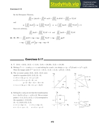

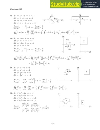
![a b
c
d
R1
R2
R3
R4
R
u
v
a b
c
d
S
u
v
2 4
-2
2
R1
R2
R3
R4
R
x
y
5 10
-2
2
S
u
v
1
2
R1
R2
R3 R
x
y
1
2
S
u
v
Exercises 9.17
Using u2
+ v2
= 4/(x2
+ y2
) we see that ∂(x, y)/∂(u, v) = −4/(u2
+ v2
)2
.
R
(x2
+ y2
)−3
dA =
S
4
u2 + v2
−3
−4
(u2 + v2)2
dA
=
1
16
1
1/3
1
1/2
(u2
+ v2
) du dv =
115
5184
17. R1: 2xy = c =⇒ v = c
R2: x2
− y2
= b =⇒ u = b
R3: 2xy = d =⇒ v = d
R4: x2
− y2
= a =⇒ u = a
∂(u, v)
∂(x, y)
=
2x −2y
2y 2x
= 4(x2
+ y2
)
=⇒
∂(x, y)
∂(u, v)
=
1
4(x2 + y2)
R
(x2
+ y2
) dA =
S
(x2
+ y2
)
1
4(x2 + y2)
dA
=
1
4
d
c
b
a
du dv =
1
4
(b − a)(d − c)
18. R1: xy = −2 =⇒ v = −2
R2: x2
− y2
= 9 =⇒ u = 9
R3: xy = 2 =⇒ v = 2
R4: x2
− y2
= 1 =⇒ u = 1
∂(u, v)
∂(x, y)
=
2x −2y
y x
= 2(x2
+ y2
)
=⇒
∂(x, y)
∂(u, v)
=
1
2(x2 + y2)
R
(x2
+ y2
) sin xy dA =
S
(x2
+ y2
) sin v
1
2(x2 + y2)
dA
=
1
2
2
−2
9
1
sin v du dv =
1
2
2
−2
8 sin v dv = 0
19. R1: y = x2
=⇒ v + u = v − u =⇒ u = 0
R2 : y = 4 − x2
=⇒ v + u = 4 − (v − u)
=⇒ v + u = 4 − v + u =⇒ v = 2
R3: x = 1 =⇒ v − u = 1 =⇒ v = 1 + u
∂(x, y)
∂(u, v)
=
−
1
2
√
v − u
1
2
√
v − u
1 1
= −
1
√
v − u
R
x
y + x2
dA =
S
√
v − u
2v
−
1
√
v − u
dA
=
1
2
1
0
2
1+u
1
v
dv du =
1
2
1
0
[ln 2 − ln(1 + u)] du
=
1
2
ln 2 −
1
2
[(1 + u) ln(1 + u) − (1 + u)]
1
0
=
1
2
ln 2 −
1
2
[2 ln 2 − 2 − (0 − 1)] =
1
2
−
1
2
ln 2
475](https://image.slidesharecdn.com/advancedengineeringmathematicssolutionsmanual-230807162553-1916df96/85/Advanced-Engineering-Mathematics-Solutions-Manual-pdf-475-320.jpg)


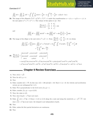
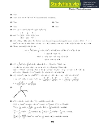
![Chapter 9 Review Exercises
37. We use spherical coordinates.
V =
2π
0
π/4
tan−1 1/3
3 sec φ
0
ρ2
sin φ dρ dφ dθ =
2π
0
π/4
tan−1 1/3
1
3
ρ3
sin φ
3 sec φ
0
dφ dθ
=
1
3
2π
0
π/4
tan−1 1/3
27 sec3
φ sin φ dφ dθ = 9
2π
0
π/4
tan−1 1/3
tan φ sec2
φ dφ dθ
= 9
2π
0
1
2
tan2
φ
π/4
tan−1 1/3
dθ =
9
2
2π
0
1 −
1
9
dθ = 8π
38. V =
2π
0
π/6
0
2
1
ρ2
sin φ dρ dφ dθ =
2π
0
π/6
0
1
3
ρ3
sin φ
2
1
dφ dθ
=
2π
0
π/6
0
8
3
sin φ −
1
3
sin φ dφ dθ =
7
3
2π
0
π/6
0
sin φ dφ dθ =
7
3
2π
0
− cos φ
π/6
0
dθ
=
7
3
2π
0
−
√
3
2
− (−1)
dθ =
7
3
1 −
√
3
2
2π =
7π
3
(2 −
√
3 )
39. 2xy + 2xy + 2xy = 6xy
40.
i j k
∂/∂x ∂/∂y ∂/∂z
x2
y xy2
2xyz
= 2xzi − 2yzj + (y2
− x2
)k
41.
∂
∂x
(2xz) −
∂
∂y
(2yz) +
∂
∂z
(y2
− x2
) = 0
42. ∇(6xy) = 6yi + 6xj
43.
C
z2
x2 + y2
ds =
2π
π
4t2
cos2 2t + sin2
2t
4 sin2
2t + 4 cos2 2t + 4 dt =
2π
π
8
√
2 t2
dt =
8
√
2
3
t3
2π
π
=
56
√
2 π3
3
44.
C
(xy + 4x) ds =
0
1
[x(2 − 2x) + 4x]
√
1 + 4 dx =
√
5
0
1
(6x − 2x2
) dx =
√
5 3x2
−
2
3
x3
0
1
= −
7
√
5
3
45. Since Py = 6x2
y = Qx, the integral is independent of path.
φx = 3x2
y2
, φ = x3
y2
+ g(y), φy = 2x3
y + g
(y) = 2x3
y − 3y2
; g(y) = −y3
; φ = x3
y2
− y3
;
(1,−2)
(0,0)
3x2
y2
dx + (2x3
y − 3y2
) dy = (x3
y2
− y3
)
(1,−2)
(0,0)
= 12
46. Let x = a cos t, y = a sin t, 0 ≤ t ≤ 2π. Then using dx = −a sin t dt, dy = a cos t dt, x2
+ y2
= a2
we have
ˇ
C
−y dx + x dy
x2 + y2
=
2π
0
1
a2
[−a sin t(−a sin t) + a cos t(a cos t)] dt =
2π
0
(sin2
t + cos2
t) dt =
2π
0
dt = 2π.
47.
C
y sin πz dx+x2
ey
dy + 3xyz dz
=
1
0
[t2
sin πt3
+ t2
et2
(2t) + 3tt2
t3
(3t2
)] dt =
1
0
(t2
sin πt3
+ 2t3
et2
+ 9t8
) dt
= −
1
3π
cos πt3
+ t9
1
0
+ 2
1
0
t3
et2
dt Integration by parts
=
2
3π
+ 1 + (t2
et2
− et2
)
1
0
=
2
3π
+ 2
482](https://image.slidesharecdn.com/advancedengineeringmathematicssolutionsmanual-230807162553-1916df96/85/Advanced-Engineering-Mathematics-Solutions-Manual-pdf-482-320.jpg)
![Chapter 9 Review Exercises
48. Parameterize C by x = cos t, y = sin t; 0 ≤ t ≤ 2π. Then
ˇ
C
F · dr =
2π
0
[4 sin t(− sin t dt) + 6 cos t(cos t) dt] =
2π
0
(6 cos2
t − 4 sin2
t) dt
=
2π
0
(10 cos2
t − 4) dt = 5t +
5
2
sin 2t − 4t
2π
0
= 2π.
Using Green’s Theorem, Qx − Py = 6 − 4 = 2 and
ˇ
C
F · dr =
R
2 dA = 2(π · 12
) = 2π.
49. Let r1 =
π
2
ti and r2 =
π
2
i + πtj for 0 ≤ t ≤ 1. Then dr1 =
π
2
i, dr2 = πj, F1 = 0,
F2 =
π
2
sin πti + πt sin
π
2
j =
π
2
sin πti + πtj,
and
W =
C1
F1 · dr1 +
C2
F2 · dr2 =
1
0
π2
t dt =
1
2
π2
t2
1
0
=
π2
2
.
50. Parameterize the line segment from (−1/2, 1/2) to (−1, 1) using y = −x as x goes from −1/2 to −1. Parameterize
the line segment from (−1, 1) to (1, 1) using y = 1 as x goes from −1 to 1. Parameterize the line segment from
(1, 1) to (1,
√
3 ) using x = 1 as y goes from 1 to
√
3 . Then
W =
C
F · dr =
−1
−1/2
F · (dxi − dxj) +
1
−1
F · (dxi) +
√
3
1
F · (dyj)
=
−1
−1/2
2
x2 + (−x)2
−
1
x2 + (−x)2
dx +
1
−1
2
x2 + 1
dx +
√
3
1
1
1 + y2
dy
=
−1
−1/2
1
2x2
dx +
1
−1
2
1 + x2
dx +
√
3
1
1
1 + y2
dy
= −
1
2x
−1
−1/2
+ 2 tan−1
x
1
−1
+ tan−1
y
√
3
1
= −
1
2
+ 2
π
2
+
π
12
=
13π − 6
12
.
51. zx = 2x, zy = 0; dS =
√
1 + 4x2 dA
S
z
xy
dS =
3
1
2
1
x2
xy
1 + 4x2 dx dy =
3
1
1
y
1
12
(1 + 4x2
)3/2
2
1
dy
=
1
12
3
1
173/2
− 53/2
y
dy =
17
√
17 − 5
√
5
12
ln y
3
1
=
17
√
17 − 5
√
5
12
ln 3
52. n = k, F · n = 3;
flux =
S
F · n dS = 3
S
dS = 3 × (area of S) = 3(1) = 3
53. The surface is g(x, y, z) = x2
+ y2
+ z2
− a2
= 0. ∇g = 2(xi + yj + zk) = 2r, n = r/|r|,
F = c∇(1/|r|) + c∇(x2
+ y2
+ z2
)−1/2
= c
−xi − yj − zk
(x2 + y2 + z2)3/2
= −cr/|r|3
F · n = −
r
|r|3
·
r
|r|
= −c
r · r
|r|4
= −c
|r|2
|r|4
= −
c
|r|2
= −
c
a2
483](https://image.slidesharecdn.com/advancedengineeringmathematicssolutionsmanual-230807162553-1916df96/85/Advanced-Engineering-Mathematics-Solutions-Manual-pdf-483-320.jpg)
![Chapter 9 Review Exercises
flux =
S
F · n dS = −
c
a2
S
dS = −
c
a2
× (area of S) = −
c
a2
(4πa2
) = −4πc
54. In Problem 53, F is not continuous at (0, 0, 0) which is in any acceptable region containing the sphere.
55. Since F = c∇(1/r), div F = ∇·(c∇(1/r)) = c∇2
(1/r) = c∇2
[(x2
+y2
+z2
)−1/2
] = 0 by Problem 37 in Section
9.7. Then, by the Divergence Theorem,
flux F =
S
F · n dS =
D
div F dV =
D
0 dV = 0.
56. Parameterize C by x = 2 cos t, y = 2 sin t, z = 5, for 0 ≤ t ≤ 2π. Then
S
(curl F · n) dS =
ˇC
F · dr =
ˇC
6x dx + 7z dy + 8y dz
=
2π
0
[12 cos t(−2 sin t) + 35(2 cos t)] dt
=
2π
0
(70 cos t − 24 sin t cos t) dt = (70 sin t − 12 sin2
t)
2π
0
= 0.
57. Identify F = −2yi + 3xj + 10zk. Then curl F = 5k. The curve C lies in the plane z = 3,
so n = k and dS = dA. Thus,
ˇ
C
F · dr =
S
(curl F) · n dS =
R
5 dA = 5 × (area of R) = 5(25π) = 125π.
58. Since curl F = 0,
ˇ
C
F · dr =
S
(curl F · n) dS =
S
0 dS = 0.
59. div f = 1 + 1 = 1 = 3;
S
F · n dS =
D
div F dV =
D
3 dV = 3 × (volume of D) = 3π
60. div F = x2
+ y2
+ z2
. Using cylindrical coordinates,
S
F · n dS =
D
div F dV =
D
(x2
+ y2
+ z2
) dV =
2π
0
1
0
1
0
(r2
+ z2
)r dz dr dθ
=
2π
0
1
0
r3
z +
1
3
rz3
1
0
dr dθ =
2π
0
1
0
r3
+
1
3
r dr dθ
=
2π
0
1
4
r4
+
1
6
r2
1
0
dθ =
2π
0
5
12
dθ =
5π
6
.
61. div F = 2x + 2(x + y) − 2y = 4x
S
F · n dS =
D
div F dV =
D
4x dV =
1
0
1−x2
0
2−z
0
4x dy dz dx
=
1
0
1−x2
0
4x(2 − z) dz dx =
1
0
1−x2
0
(8x − 4xz) dz dx
=
1
0
(8xz − 2xz2
)
1−x2
0
dx =
1
0
[8x(1 − x2
) − 2x(1 − x2
)2
] dx
=
−2(1 − x2
)2
+
1
3
(1 − x2
)3
1
0
=
5
3
484](https://image.slidesharecdn.com/advancedengineeringmathematicssolutionsmanual-230807162553-1916df96/85/Advanced-Engineering-Mathematics-Solutions-Manual-pdf-484-320.jpg)
![Chapter 9 Review Exercises
obtain (z − a)2
− z2
= 1 − a2
or −2az + a2
= 1 − a2
. Thus, the spheres intersect on the plane z = a − 1/2a.
The region of integration is x2
+ y2
+ (a − 1/2a)2
= a2
or r2
= 1 − 1/4a2
. The area is
A = a
2π
0
√
1−1/4a2
0
(a2
− r2
)−1/r
r dr dθ = 2πa[−(a2
− r2
)1/2
]
√
1−1/4a2
0
= 2πa
a −
a2
− 1 −
1
4a2
1/2
= 2πa a −
a −
1
2a
2
1/2
= π.
66. (a) Both states span 7 degrees of longitude and 4 degrees of latitude, but Colorado is larger because it lies
to the south of Wyoming. Lines of longitude converge as they go north, so the east-west dimensions of
Wyoming are shorter than those of Colorado.
(b) We use the function f(x, y) = R2 − x2 − y2 to describe the northern
hemisphere, where R ≈ 3960 miles is the radius of the Earth. We need to
compute the surface area over a polar rectangle P of the form θ1 ≤ θ ≤ θ2,
R cos φ2 ≤ r ≤ R cos φ1. We have
fx =
−x
R2 − x2 − y2
and fy =
−y
R2 − x2 − y2
so that
1 + f2
x + f2
y =
1 +
x2 + y2
R2 − x2 − y2
=
R
√
R2 − r2
.
Thus
A =
P
1 + f2
x + f2
y dA =
θ2
θ1
R cos φ1
R cos φ2
R
√
R2 − r2
r dr dθ
= (θ2 − θ1)R R2 − r2
R cos φ2
R cos φ1
= (θ2 − θ1)R2
(sin φ2 − sin φ1).
The ratio of Wyoming to Colorado is then
sin 45◦
− sin 41◦
sin 41◦ − sin 37◦
≈ 0.941. Thus Wyoming is about 6%
smaller
than Colorado.
(c) 97,914/104,247 ≈ 0.939, which is close to the theoretical value of 0.941. (Our formula for the area says that
the area of Colorado is approximately 103,924 square miles, while the area of Wyoming is approximately
97,801 square miles.)
486](https://image.slidesharecdn.com/advancedengineeringmathematicssolutionsmanual-230807162553-1916df96/85/Advanced-Engineering-Mathematics-Solutions-Manual-pdf-486-320.jpg)


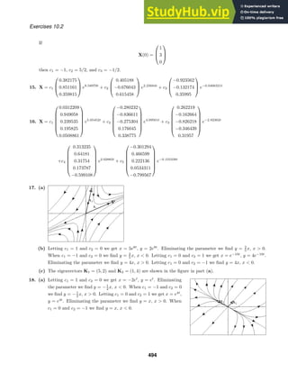


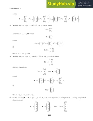
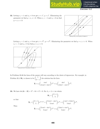


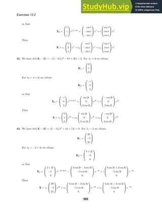
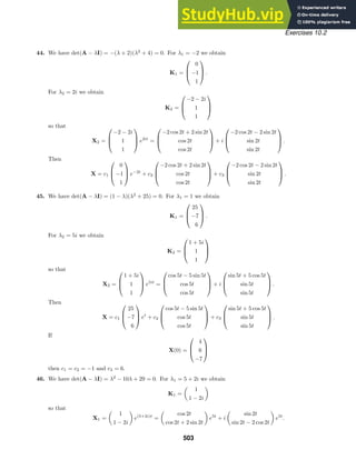
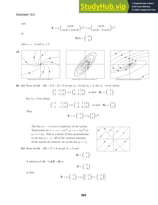
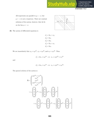


![Exercises 10.5
25. From Problems 23 and 24 and equation (1) in the text
X = eAt
C = PeDt
P−1
C =
e3t
e5t
e3t
3e5t
e3t
0
0 e5t
3
2 e−3t
−1
2 e−3t
−1
2 e−5t 1
2 e−5t
c1
c2
=
3
2 e3t
− 1
2 e5t
−1
2 e3t
+ 1
2 e5t
3
2 e3t
− 3
2 e5t
−1
2 e3t
+ 3
2 e5t
c1
c2
.
26. From Problems 23 and 24 and equation (1) in the text
X = eAt
C = PeDt
P−1
C =
−et
e3t
et
e3t
et
0
0 e3t
−1
2 e−t 1
2 e−t
1
2 e3t 1
2 e−3t
c1
c2
=
1
2 et
+ 1
2 e9t
−1
2 et
+ 1
2 e3t
−1
2 et
+ 1
2 e9t 1
2 et
+ 1
2 e3t
c1
c2
.
27. (a) The following commands can be used in Mathematica:
A={{4, 2},{3, 3}};
c={c1, c2};
m=MatrixExp[A t];
sol=Expand[m.c]
Collect[sol, {c1, c2}] // MatrixForm
The output gives
x(t) = c1
2
5
et
+
3
5
e6t
+ c2
−
2
5
et
+
2
5
e6t
y(t) = c1
−
3
5
et
+
3
5
e6t
+ c2
3
5
et
+
2
5
e6t
.
The eigenvalues are 1 and 6 with corresponding eigenvectors
−2
3
and
1
1
,
so the solution of the system is
X(t) = b1
−2
3
et
+ b2
1
1
e6t
or
x(t) = −2b1et
+ b2e6t
y(t) = 3b1et
+ b2e6t
.
If we replace b1 with −1
5 c1 + 1
5 c2 and b2 with 3
5 c1 + 2
5 c2, we obtain the solution found using the matrix
exponential.
(b) x(t) = c1e−2t
cos t − (c1 + c2)e−2t
sin t
y(t) = c2e−2t
cos t + (2c1 + c2)e−2t
sin t
28. x(t) = c1(3e−2t
− 2e−t
) + c3(−6e−2t
+ 6e−t
)
y(t) = c2(4e−2t
− 3e−t
) + c4(4e−2t
− 4e−t
)
z(t) = c1(e−2t
− e−t
) + c3(−2e−2t
+ 3e−t
)
w(t) = c2(−3e−2t
+ 3e−t
) + c4(−3e−2t
+ 4e−t
)
528](https://image.slidesharecdn.com/advancedengineeringmathematicssolutionsmanual-230807162553-1916df96/85/Advanced-Engineering-Mathematics-Solutions-Manual-pdf-528-320.jpg)
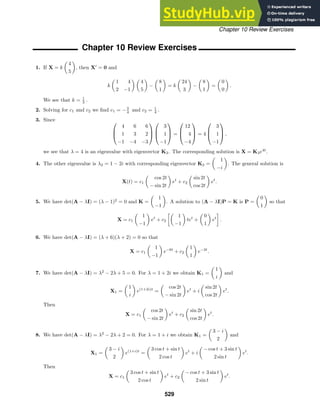

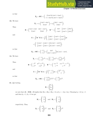


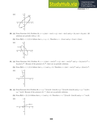
![Exercises 11.1
23. Switching to polar coordinates,
dr
dt
=
1
r
x
dx
dt
+ y
dy
dt
=
1
r
(−xy − x2
r4
+ xy − y2
r4
) = −r5
dθ
dt
=
1
r2
−y
dx
dt
+ x
dy
dt
=
1
r2
(y2
+ xyr4
+ x2
− xyr4
) = 1 .
If we use separation of variables on
dr
dt
= −r5
we obtain
r =
1
4t + c1
1/4
and θ = t + c2.
Since X(0) = (4, 0), r = 4 and θ = 0 when t = 0. It follows that c2 = 0 and c1 =
1
256
. The final solution may
be written as
r =
4
4
√
1024t + 1
, θ = t
and so the solution spirals toward the origin as t increases.
24. Switching to polar coordinates,
dr
dt
=
1
r
x
dx
dt
+ y
dy
dt
=
1
r
(xy − x2
r2
− xy + y2
r2
) = r3
dθ
dt
=
1
r2
−y
dx
dt
+ x
dy
dt
=
1
r2
(−y2
− xyr2
− x2
+ xyr2
) = −1 .
If we use separation of variables, it follows that
r =
1
√
−2t + c1
and θ = −t + c2.
Since X(0) = (4, 0), r = 4 and θ = 0 when t = 0. It follows that c2 = 0 and c1 = 1
16 . The final solution may be
written as
r =
4
√
1 − 32t
, θ = −t.
Note that r → ∞ as t →
1
32
−
. Because 0 ≤ t ≤ 1
32 , the curve is not a spiral.
25. Switching to polar coordinates,
dr
dt
=
1
r
x
dx
dt
+ y
dy
dt
=
1
r
[−xy + x2
(1 − r2
) + xy + y2
(1 − r2
)] = r(1 − r2
)
dθ
dt
=
1
r2
−y
dx
dt
+ x
dy
dt
=
1
r2
[y2
− xy(1 − r2
) + x2
+ xy(1 − r2
)] = 1.
Now
dr
dt
= r − r3
or
dr
dt
− r = −r3
is a Bernoulli differential equation. Following the procedure in Section 2.5
of the text, we let w = r−2
so that w
= −2r−3 dr
dt
. Therefore w
+ 2w = 2, a linear first order differential
equation. It follows that w = 1 + c1e−2t
and so r2
=
1
1 + c1e−2t
. The general solution may be written as
r =
1
√
1 + c1e−2t
, θ = t + c2.
If X(0) = (1, 0), r = 1 and θ = 0 when t = 0. Therefore c1 = 0 = c2 and so x = r cos t = cos t and
y = r sin t = sin t. This solution generates the circle r = 1. If X(0) = (2, 0), r = 2 and θ = 0 when t = 0.
536](https://image.slidesharecdn.com/advancedengineeringmathematicssolutionsmanual-230807162553-1916df96/85/Advanced-Engineering-Mathematics-Solutions-Manual-pdf-536-320.jpg)

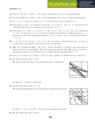
![Exercises 11.3
(b) From the graph, X1 appears to be an unstable spiral point.
(c) Since τ = 0.2, ∆ = 0.03, and τ2 − 4∆ = −0.08, (0, 0) is an unstable spiral point.
26. (a) The critical point is X1 = (1, 1).
(b) From the graph, X1 appears to be a center.
(c) Since τ = 0 and ∆ = 1, (0, 0) is a center.
Exercises 11.3
1. Switching to polar coordinates,
dr
dt
=
1
r
x
dx
dt
+ y
dy
dt
=
1
r
(αx2
− βxy + xy2
+ βxy + αy2
− xy2
) =
1
r
αr2
= αr.
Therefore r = ceαt
and so r → 0 if and only if α 0.
2. The differential equation
dr
dt
= αr(5 − r) is a logistic differential equation. [See Section 2.8, (4) and (5).] It
follows that
r =
5
1 + c1e−5αt
and θ = −t + c2.
If α 0, r → 5 as t → +∞ and so the critical point (0, 0) is unstable. If α 0, r → 0 as t → +∞ and so (0, 0)
is asymptotically stable.
3. The critical points are x = 0 and x = n + 1. Since g
(x) = k(n + 1) − 2kx, g
(0) = k(n + 1) 0 and
g
(n + 1) = −k(n + 1) 0. Therefore x = 0 is unstable while x = n + 1 is asymptotically stable. See
Theorem 11.2.
4. Note that x = k is the only critical point since ln(x/k) is not defined at x = 0. Since g
(x) = −k − k ln(x/k),
g
(k) = −k 0. Therefore x = k is an asymptotically stable critical point by Theorem 11.2.
5. The only critical point is T = T0. Since g
(T) = k, g
(T0) = k 0. Therefore T = T0 is unstable by
Theorem 11.2.
6. The only critical point is v = mg/k. Now g(v) = g − (k/m)v and so g
(v) = −k/m 0. Therefore v = mg/k is
an asymptotically stable critical point by Theorem 11.2.
541](https://image.slidesharecdn.com/advancedengineeringmathematicssolutionsmanual-230807162553-1916df96/85/Advanced-Engineering-Mathematics-Solutions-Manual-pdf-541-320.jpg)

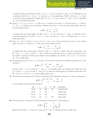
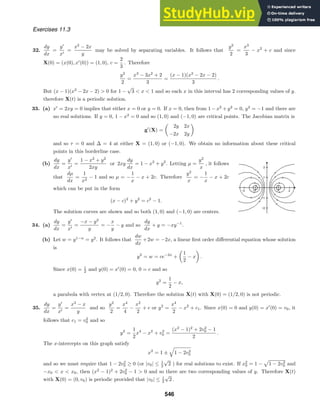
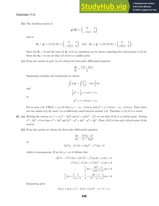
![Exercises 11.4
or
x
u + 1
u
(u2
− u + 1) = c2
x
y + x
y
y2
x2
−
y
x
+ 1
= c2
(xy + x2
)(y2
− xy + x2
) = c2x2
y
xy3
+ x4
= c2x2
y
x3
+ y2
= 3c3xy.
(c) We see from the graph that (0, 0) is unstable. It is not possible to classify
the critical point as a node, saddle, center, or spiral point.
Exercises 11.4
1. We are given that x(0) = θ(0) =
π
3
and y(0) = θ
(0) = w0. Since y2
=
2g
l
cos x + c, w2
0 =
2g
l
cos
π
3
+ c =
g
l
+ c
and so c = w2
0 −
g
l
. Therefore
y2
=
2g
l
cos x −
1
2
+
l
2g
w2
0
and the x-intercepts occur where cos x =
1
2
−
l
2g
w2
0 and so
1
2
−
l
2g
w2
0 must be greater than −1 for solutions to
exist. This condition is equivalent to |w0|
3g
l
.
2. (a) Since y2
=
2g
l
cos x+c, x(0) = θ(0) = θ0 and y(0) = θ
(0) = 0, c = −
2g
l
cos θ0 and so y2
=
2g
l
(cos θ−cos θ0).
When θ = −θ0, y2
=
2g
l
(cos(−θ0) − cos(θ0)) = 0. Therefore y =
dθ
dt
= 0 when θ = θ0.
(b) Since y =
dθ
dt
and θ is decreasing between the time when θ = θ0, t = 0, and θ = −θ0, that is, t = T,
dθ
dt
= −
2g
l
cos θ − cos θ0 .
Therefore
dt
dθ
= −
l
2g
1
√
cos θ − cos θ0
and so
T = −
l
2g
θ=−θ0
θ=θ0
1
√
cos θ − cos θ0
dθ =
l
2g
θ0
−θ0
1
√
cos θ − cos θ0
dθ.
3. The corresponding plane autonomous system is
x
= y, y
= −g
f
(x)
1 + [f(x)]2
−
β
m
y
549](https://image.slidesharecdn.com/advancedengineeringmathematicssolutionsmanual-230807162553-1916df96/85/Advanced-Engineering-Mathematics-Solutions-Manual-pdf-549-320.jpg)
![Exercises 11.4
and
∂
∂x
−g
f
(x)
1 + [f(x)]2
−
β
m
y
= −g
(1 + [f
(x)]2
)f
(x) − f
(x)2f
(x)f
(x)
(1 + [f(x)]2)2
.
If X1 = (x1, y1) is a critical point, y1 = 0 and f
(x1) = 0. The Jacobian at this critical point is therefore
g
(X1) =
0 1
−gf
(x1) − β
m
.
4. When β = 0 the Jacobian matrix is
0 1
−gf
(x1) 0
which has complex eigenvalues λ = ±
gf(x1) i. The approximating linear system with x
(0) = 0 has solution
x(t) = x(0) cos
gf(x1) t
and period 2π/
gf(x1) . Therefore p ≈ 2π/
gf(x1) for the actual solution.
5. (a) If f(x) =
x2
2
, f
(x) = x and so
dy
dx
=
y
x
= −g
x
1 + x2
1
y
.
We may separate variables to show that y2
= −g ln(1 + x2
) + c. But x(0) = x0 and y(0) = x
(0) = v0.
Therefore c = v2
0 + g ln(1 + x2
0) and so
y2
= v2
0 − g ln
1 + x2
1 + x2
0
.
Now
v2
0 − g ln
1 + x2
1 + x2
0
≥ 0 if and only if x2
≤ ev2
0/g
(1 + x2
0) − 1.
Therefore, if |x| ≤ [ev2
0/g
(1 + x2
0) − 1]1/2
, there are two values of y for a given value of x and so the solution
is periodic.
(b) Since z =
x2
2
, the maximum height occurs at the largest value of x on the cycle. From (a), xmax =
[ev2
0/g
(1 + x2
0) − 1]1/2
and so
zmax =
x2
max
2
=
1
2
[ev2
0/g
(1 + x2
0) − 1].
6. (a) If f(x) = cosh x, f
(x) = sinh x and [f
(x)]2
+ 1 = sinh2
x + 1 = cosh2
x. Therefore
dy
dx
=
y
x
= −g
sinh x
cosh2
x
1
y
.
We may separate variables to show that y2
=
2g
cosh x
+ c. But x(0) = x0 and y(0) = x
(0) = v0. Therefore
c = v2
0 −
2g
cosh x0
and so
y2
=
2g
cosh x
−
2g
cosh x0
+ v2
0.
Now
2g
cosh x
−
2g
cosh x0
+ v2
0 ≥ 0 if and only if cosh x ≤
2g cosh x0
2g − v2
0 cosh x0
550](https://image.slidesharecdn.com/advancedengineeringmathematicssolutionsmanual-230807162553-1916df96/85/Advanced-Engineering-Mathematics-Solutions-Manual-pdf-550-320.jpg)
![x(t)
y(t)
t
x,y
20 40 60 80 100
5
10
Exercises 11.4
and the solution to this inequality is an interval [−a, a]. Therefore each x in (−a, a) has two corresponding
values of y and so the solution is periodic.
(b) Since z = cosh x, the maximum height occurs at the largest value of x on the cycle. From (a), xmax = a
where cosh a =
2g cosh x0
2g − v2
0 cosh x0
. Therefore
zmax =
2g cosh x0
2g − v2
0 cosh x0
.
7. If xm x1 xn, then F(x1) F(xm) = F(xn). Letting x = x1,
G(y) =
c0
F(x1)
=
F(xm)G(a/b)
F(x1)
G(a/b).
Therefore from Figure 11.35(b), G(y) =
c0
F(x1)
has two solutions y1 and y2 that satisfy y1 a/b y2.
8. From (i) when y = a/b, xn is taken on at some time t. From (iii) if x xn there is no corresponding value of
y. Therefore the maximum number of predators is xn and xn occurs when y = a/b.
9. (a) In the Lotka-Volterra Model the average number of predators is d/c and the average number of prey is a/b.
But
x
= −ax + bxy − 1x = −(a + 1)x + bxy
y
= −cxy + dy − 2y = −cxy + (d − 2)y
and so the new critical point in the first quadrant is (d/c − 2/c, a/b + 1/b).
(b) The average number of predators d/c − 2/c has decreased while the average number of prey a/b + 1/b has
increased. The fishery science model is consistent with Volterra’s principle.
10. (a) Solving
x(−0.1 + 0.02y) = 0
y(0.2 − 0.025x) = 0
in the first quadrant we obtain the critical point
(8, 5). The graphs are plotted using x(0) = 7
and y(0) = 4.
(b) The graph in part (a) was obtained using NDSolve in Mathematica. We see that the period is around
40. Since x(0) = 7, we use the FindRoot equation solver in Mathematica to approximate the solution of
x(t) = 7 for t near 40. From this we see that the period is more closely approximated by t = 44.65.
11. Solving
x(20 − 0.4x − 0.3y) = 0
y(10 − 0.1y − 0.3x) = 0
we see that critical points are (0, 0), (0, 100), (50, 0), and (20, 40). The Jacobian matrix is
g
(X) =
0.08(20 − 0.8x − 0.3y) −0.024x
−0.018y 0.06(10 − 0.2y − 0.3x)
and so
A1 = g
((0, 0)) =
1.6 0
0 0.6
A3 = g
((50, 0)) =
−1.6 −1.2
0 −0.3
A2 = g
((0, 100)) =
−0.8 0
−1.8 −0.6
A4 = g
((20, 40)) =
−0.64 −0.48
−0.72 −0.24
.
551](https://image.slidesharecdn.com/advancedengineeringmathematicssolutionsmanual-230807162553-1916df96/85/Advanced-Engineering-Mathematics-Solutions-Manual-pdf-551-320.jpg)
![Exercises 11.4
Since det(A1) = ∆1 = 0.96 0, τ = 2.2 0, and τ2
1 − 4∆1 = 1 0, we see that (0, 0) is an unstable node.
Since det(A2) = ∆2 = 0.48 0, τ = −1.4 0, and τ2
2 − 4∆2 = 0.04 0, we see that (0, 100) is a stable node.
Since det(A3) = ∆3 = 0.48 0, τ = −1.9 0, and τ2
3 − 4∆3 = 1.69 0, we see that (50, 0) is a stable node.
Since det(A4) = −0.192 0 we see that (20, 40) is a saddle point.
12. ∆ = r1r2, τ = r1 + r2 and τ2
− 4∆ = (r1 + r2)2
− 4r1r2 = (r1 − r2)2
. Therefore when r1 = r2, (0, 0) is an
unstable node.
13. For X = (K1, 0), τ = −r1 + r2
1 −
K1
K2
α21
and ∆ = −r1r2
1 −
K1
K2
α21
. If we let c = 1 −
K1
K2
α21,
τ2
− 4∆ = (cr2 + r1)2
0. Now if k1
K2
α21
, c 0 and so τ 0, ∆ 0. Therefore (K1, 0) is a stable node. If
K1
K2
α21
, c 0 and so ∆ 0. In this case (K1, 0) is a saddle point.
14. (x̂, ŷ) is a stable node if and only if
K1
α12
K2 and
K2
α21
K1. [See Figure 11.38(a) in the text.] From Problem
12, (0.0) is an unstable node and from Problem 13, since K1
K2
α21
, (K1, 0) is a saddle point. Finally, when
K2
K1
α12
, (0, K2) is a saddle point. This is Problem 12 with the roles of 1 and 2 interchanged. Therefore
(0, 0), (K1, 0), and (0, K2) are unstable.
15.
K1
α12
K2 K1α21 and so α12α21 1. Therefore ∆ = (1 − α12α21)x̂ŷ
r1r2
K1K2
0 and so (x̂, ŷ) is a saddle
point.
16. (a) The corresponding plane autonomous system is
x
= y, y
=
−g
l
sin x −
β
ml
y
and so critical points must satisfy both y = 0 and sin x = 0. Therefore (±nπ, 0) are critical points.
(b) The Jacobian matrix
0 1
−
g
l
cos x −
β
ml
has trace τ = −
β
ml
and determinant ∆ =
g
l
0 at (0, 0). Therefore
τ2
− 4∆ =
β2
m2l2
− 4
g
l
=
β2
− 4glm2
m2l2
.
We may conclude that (0, 0) is a stable spiral point provided β2
− 4glm2
0 or β 2m
√
gl .
17. (a) The corresponding plane autonomous system is
x = y, y
= −
β
m
y|y| −
k
m
x
and so a critical point must satisfy both y = 0 and x = 0. Therefore (0, 0) is the unique critical point.
(b) The Jacobian matrix is
0 1
−
k
m
−
β
m
2|y|
552](https://image.slidesharecdn.com/advancedengineeringmathematicssolutionsmanual-230807162553-1916df96/85/Advanced-Engineering-Mathematics-Solutions-Manual-pdf-552-320.jpg)
![Exercises 11.4
and so τ = 0 and ∆ =
k
m
0. Therefore (0, 0) is a center, stable spiral point, or an unstable spiral point.
Physical considerations suggest that (0, 0) must be asymptotically stable and so (0, 0) must be a stable
spiral point.
18. (a) The magnitude of the frictional force between the bead and the wire is µ(mg cos θ) for some µ 0. The
component of this frictional force in the x-direction is
(µmg cos θ) cos θ = µmg cos2
θ.
But
cos θ =
1
1 + [f(x)]2
and so µmg cos2
θ =
µmg
1 + [f(x)]2
.
It follows from Newton’s Second Law that
mx
= −mg
f
(x)
1 + [f(x)]2
− βx
+ mg
µ
1 + [f(x)]2
and so
x
= g
µ − f
(x)
1 + [f(x)]2
−
β
m
x
.
(b) A critical point (x, y) must satisfy y = 0 and f
(x) = µ. Therefore critical points occur at (x1, 0) where
f
(x1) = µ. The Jacobian matrix of the plane autonomous system is
g
(X) =
0 1
g
(1 + [f
(x)]2
)(−f
(x)) − (µ − f
(x))2f
(x)f
(x)
(1 + [f(x)]2)2
−
β
m
and so at a critical point X1,
g
(X) =
0 1
−gf
(x1)
1 + µ2
−
β
m
.
Therefore τ = −
β
m
0 and ∆ =
gf
(x1)
1 + µ2
. When f
(x1) 0, ∆ 0 and so a saddle point occurs. When
f
(x1) 0 and
τ2
− 4∆ =
β2
m2
− 4g
f
(x1)
1 + µ2
0,
(x1, 0) is a stable spiral point. This condition may also be written as
β2
4gm2 f
(x1)
1 + µ2
.
19.
dy
dx
=
y
x
= −
f(x)
y
and so using separation of variables,
y2
2
= −
x
0
f(µ) dµ + c or y2
+ 2F(x) = c. We may
conclude that for a given value of x there are at most two corresponding values of y. If (0, 0) were a stable spiral
point there would exist an x with more than two corresponding values of y. Note that the condition f(0) = 0
is required for (0, 0) to be a critical point of the corresponding plane autonomous system x
= y, y
= −f(x).
20. (a) x
= x(−a + by) = 0 implies that x = 0 or y = a/b. If x = 0, then, from
−cxy +
r
K
y(K − y) = 0,
y = 0 or K. Therefore (0, 0) and (0, K) are critical points. If ŷ = a/b, then
ŷ −cx +
r
K
(K − ŷ) = 0.
553](https://image.slidesharecdn.com/advancedengineeringmathematicssolutionsmanual-230807162553-1916df96/85/Advanced-Engineering-Mathematics-Solutions-Manual-pdf-553-320.jpg)
![Exercises 11.4
The corresponding value of x, x = x̂, therefore satisfies the equation cx̂ =
r
K
(K − ŷ).
(b) The Jacobian matrix is
g
(X) =
−a + by bx
−cy −cx +
r
K
(K − 2y)
and so at X1 = (0, 0), ∆ = −ar 0. For X1 = (0, K), ∆ = n(Kb − a) = −rb
K −
a
b
. Since we are given
that K
a
b
, ∆ 0 in this case. Therefore (0, 0) and (0, K) are each saddle points. For X1 = (x̂, ŷ) where
ŷ =
a
b
and cx̂ =
r
K
(K − ŷ), we may write the Jacobian matrix as
g
((x̂, ŷ)) =
0 bx̂
−cŷ −
r
K
ŷ
and so τ = −
r
K
ŷ 0 and ∆ = bcx̂ŷ 0. Therefore (x̂, ŷ) is a stable critical point and so it is either a
stable node (perhaps degenerate) or a stable spiral point.
(c) Write
τ2
− 4∆ =
r2
K2
ŷ2
− 4bcx̂ŷ = ŷ
r2
K2
ŷ − 4bcx̂ = ŷ
r2
K2
ŷ − 4b
r
K
(K − ŷ)
using
cx̂ =
r
K
(K − ŷ) =
r
K
ŷ
r
K
+ 4b
ŷ − 4bK .
Therefore τ2
− 4∆ 0 if and only if
ŷ
4bK
r
K + 4b
=
4bK2
r + 4bK
.
Note that
4bK2
r + 4bK
=
4bK
r + 4bK
· K ≈ K
where K is large, and ŷ =
a
b
K. Therefore τ2
− 4∆ 0 when K is large and a stable spiral point will
result.
21. The equation
x
= α
y
1 + y
x − x = x
αy
1 + y
− 1
= 0
implies that x = 0 or y =
1
α − 1
. When α 0, ŷ =
1
α − 1
0. If x = 0, then from the differential equation for
y
, y = β. On the other hand, if ŷ =
1
α − 1
,
ŷ
1 + ŷ
=
1
α
and so
1
α
x̂ −
1
α − 1
+ β = 0. It follows that
x̂ = α
β −
1
α − 1
=
α
α − 1
[(α − 1)β − 1]
and if β(α − 1) 1, x̂ 0. Therefore (x̂, ŷ) is the unique critical point in the first quadrant. The Jacobian
matrix is
g
(X) =
α
y
y + 1
− 1
αx
(1 + y)2
−
y
1 + y
−x
(1 + y)2
− 1
554](https://image.slidesharecdn.com/advancedengineeringmathematicssolutionsmanual-230807162553-1916df96/85/Advanced-Engineering-Mathematics-Solutions-Manual-pdf-554-320.jpg)
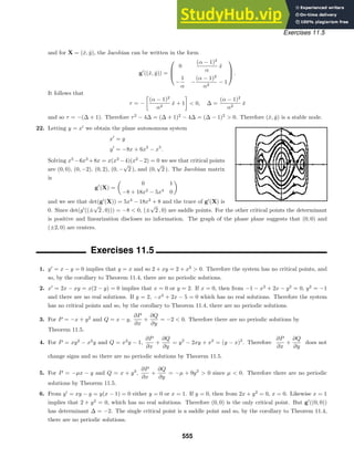
![Exercises 11.5
7. The corresponding plane autonomous system is x
= y, y
= 2x − y4
. Therefore (0, 0) is the only critical point.
But g
((0, 0)) has determinant ∆ = −2 0. The single critical point is a saddle point and so, by the corollary
to Theorem 11.4, there are no periodic solutions.
8. The corresponding plane autonomous system is
x
= y, y
= −x +
1
2
+ 3y2
y − x2
and so
∂P
∂x
+
∂Q
∂y
= 0 +
1
2
+ 9y2
0. Therefore there are no periodic solutions by Theorem 11.5.
9. For δ(x, y) = eax+by
,
∂
∂x
(δP) +
∂
∂y
(δQ) can be simplified to
eax+by
[−bx2
− 2ax + axy + (2b + 1)y].
Setting a = 0 and b = −1/2,
∂
∂
(δP) +
∂
∂y
(δQ) =
1
2
x2
e− 1
2 y
which does not change signs. Therefore by Theorem 11.6 there are no periodic solutions.
10. For δ(x, y) = ax2
+ by2
,
∂
∂x
(δP) +
∂
∂y
(δQ) can be simplified to
−5ax4
− 3bx2
y2
+ 10(a − b)x2
y.
Setting a = b = 1,
∂
∂x
(δP) +
∂
∂y
(δQ) = −5x4
− 3x2
y2
which does not change signs. Therefore by Theorem 11.6 there are no periodic solutions.
11. For P = x(1 − x2
− 3y2
) and Q = y(3 − x2
− 3y2
),
∂P
∂x
+
∂Q
∂y
= 4(1 − x2
− 3y2
) and so
∂P
∂x
+
∂Q
∂y
0
for x2
+ 3y2
1. Therefore there are no periodic solutions in the elliptical region x2
+ 3y2
1.
12. The corresponding plane autonomous system is x
= y, y
= g(x, y) and so
∂P
∂x
+
∂Q
∂y
=
∂g
∂y
=
∂g
∂x
= 0
in the region R. Therefore
∂P
∂x
+
∂Q
∂y
cannot change signs and so there are no periodic solutions by
Theorem 11.5.
13. For δ(x, y) =
1
xy
, δP = −
a
y
+ b, δQ = −c +
r
K
1
x
(K − y) and so
∂(δP)
∂x
+
∂(δQ)
∂y
= −
r
Kx
0
in the first quadrant. By Theorem 11.6, there are no periodic solutions in the first quadrant.
14. If n = (−2x, −2y),
V · n = 2xy + 2x2
ex+y
− 2xy + 2y2
ex+y
= 2(x2
+ y2
)ex+y
≥ 0.
Therefore any circular region of the form x2
+ y2
≤ r2
is an invariant region by Theorem 11.7.
15. If n = (−2x, −2y),
V · n = 2x2
− 4xy + 2y2
+ 2y4
= 2(x − y)2
+ 2y4
≥ 0.
556](https://image.slidesharecdn.com/advancedengineeringmathematicssolutionsmanual-230807162553-1916df96/85/Advanced-Engineering-Mathematics-Solutions-Manual-pdf-556-320.jpg)
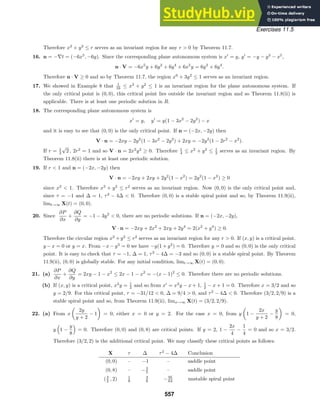

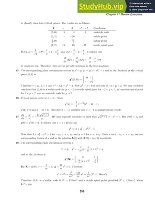
![12 Orthogonal Functions and Fourier Series
Exercises 12.1
1. 592
2
−2
xx2
dx =
1
4
x4
2
−2
= 0
2.
1
−1
x3
(x2
+ 1)dx =
1
6
x6
1
−1
+
1
4
x4
1
−1
= 0
3.
2
0
ex
(xe−x
− e−x
)dx =
2
0
(x − 1)dx =
1
2
x2
− x
2
0
= 0
4.
π
0
cos x sin2
x dx =
1
3
sin3
x
π
0
= 0
5.
π/2
−π/2
x cos 2x dx =
1
2
1
2
cos 2x + x sin 2x
π/2
−π/2
= 0
6.
5π/4
π/4
ex
sin x dx =
1
2
ex
sin x −
1
2
ex
cos x
5π/4
π/4
= 0
7. For m = n
π/2
0
sin(2n + 1)x sin(2m + 1)x dx
=
1
2
π/2
0
[cos 2(n − m)x − cos 2(n + m + 1)x] dx
=
1
4(n − m)
sin 2(n − m)x
π/2
0
−
1
4(n + m + 1)
sin 2(n + m + 1)x
π/2
0
= 0.
For m = n π/2
0
sin2
(2n+1)x dx =
π/2
0
1
2
−
1
2
cos 2(2n + 1)x
dx
=
1
2
x
π/2
0
−
1
4(2n + 1)
sin 2(2n + 1)x
π/2
0
=
π
4
so that
sin(2n + 1)x =
1
2
√
π .
562](https://image.slidesharecdn.com/advancedengineeringmathematicssolutionsmanual-230807162553-1916df96/85/Advanced-Engineering-Mathematics-Solutions-Manual-pdf-562-320.jpg)
![Exercises 12.1
8. For m = n
π/2
0
cos(2n + 1)x cos(2m + 1)x dx
=
1
2
π/2
0
[cos 2(n − m)x + cos 2(n + m + 1)x] dx
=
1
4(n − m)
sin 2(n − m)x
π/2
0
+
1
4(n + m + 1)
sin 2(n + m + 1)x
π/2
0
= 0.
For m = n
π/2
0
cos2
(2n + 1)x dx =
π/2
0
1
2
+
1
2
cos 2(2n + 1)x
dx
=
1
2
x
π/2
0
+
1
4(2n + 1)
sin 2(2n + 1)x
π/2
0
=
π
4
so that
cos(2n + 1)x =
1
2
√
π .
9. For m = n
π
0
sin nx sin mx dx =
1
2
π
0
[cos(n − m)x − cos(n + m)x] dx
=
1
2(n − m)
sin(n − m)x
π
0
−
1
2(n + m)
sin 2(n + m)x
π
0
= 0.
For m = n π
0
sin2
nx dx =
π
0
1
2
−
1
2
cos 2nx
dx =
1
2
x
π
0
−
1
4n
sin 2nx
π
0
=
π
2
so that
sin nx =
π
2
.
10. For m = n
p
0
sin
nπ
p
x sin
mπ
p
x dx =
1
2
p
0
cos
(n − m)π
p
x − cos
(n + m)π
p
x
dx
=
p
2(n − m)π
sin
(n − m)π
p
x
p
0
−
p
2(n + m)π
sin
(n + m)π
p
x
p
0
= 0.
For m = n p
0
sin2 nπ
p
x dx =
p
0
1
2
−
1
2
cos
2nπ
p
x
dx =
1
2
x
p
0
−
p
4nπ
sin
2nπ
p
x
p
0
=
p
2
so that
sin
nπ
p
x =
p
2
.
563](https://image.slidesharecdn.com/advancedengineeringmathematicssolutionsmanual-230807162553-1916df96/85/Advanced-Engineering-Mathematics-Solutions-Manual-pdf-563-320.jpg)
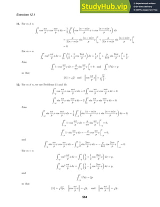
![Exercises 12.1
16. Using the facts that φ0 and φ1 are orthogonal to φn for n 1, we have
b
a
(αx + β)φn(x) dx = α
b
a
xφn(x) dx + β
b
a
1 · φn(x) dx
= α
b
a
φ1(x)φn(x) dx + β
b
a
φ0(x)φn(x) dx
= α · 0 + β · 0 = 0
for n = 2, 3, 4, . . . .
17. Using the fact that φn and φm are orthogonal for n = m we have
φm(x) + φn(x)
2
=
b
a
[φm(x) + φn(x)]2
dx
b
a
φ2
m(x) + 2φm(x)φn(x) + φ2
n(x)
dx
=
b
a
φ2
m(x)dx + 2
b
a
φm(x)φn(x)dx +
b
a
φ2
n(x) dx
= φm(x)
2
+ φn(x)
2
.
18. Setting
0 =
2
−2
f3(x)f1(x) dx =
2
−2
x2
+ c1x3
+ c2x4
dx =
16
3
+
64
5
c2
and
0 =
2
−2
f3(x)f2(x) dx =
2
−2
x3
+ c1x4
+ c2x5
dx =
64
5
c1
we obtain c1 = 0 and c2 = −5/12.
19. Since sin nx is an odd function on [−π, π],
(1, sin nx) =
π
−π
sin nx dx = 0
and f(x) = 1 is orthogonal to every member of {sin nx}. Thus {sin nx} is not complete.
20. (f1 + f2, f3) =
b
a
[f1(x) + f2(x)]f3(x) dx =
b
a
f1(x)f3(x) dx +
b
a
f2(x)f3(x) dx = (f1, f3) + (f2, f3)
21. (a) The fundamental period is 2π/2π = 1.
(b) The fundamental period is 2π/(4/L) = 1
2 πL.
(c) The fundamental period of sin x + sin 2x is 2π.
(d) The fundamental period of sin 2x + cos 4x is 2π/2 = π.
(e) The fundamental period of sin 3x+cos 4x is 2π since the smallest integer multiples of 2π/3 and 2π/4 = π/2
that are equal are 3 and 4, respectively.
(f) The fundamental period of f(x) is 2π/(nπ/p) = 2p/n.
566](https://image.slidesharecdn.com/advancedengineeringmathematicssolutionsmanual-230807162553-1916df96/85/Advanced-Engineering-Mathematics-Solutions-Manual-pdf-566-320.jpg)
![Exercises 12.2
Exercises 12.2
1. a0 =
1
π
π
−π
f(x) dx =
1
π
π
0
1 dx = 1
an =
1
π
π
−π
f(x) cos
nπ
π
x dx =
1
π
π
0
cos nx dx = 0
bn =
1
π
π
−π
f(x) sin
nπ
π
x dx =
1
π
π
0
sin nx dx =
1
nπ
(1 − cos nπ) =
1
nπ
[1 − (−1)n
]
f(x) =
1
2
+
1
π
∞
n=1
1 − (−1)n
n
sin nx
2. a0 =
1
π
π
−π
f(x) dx =
1
π
0
−π
−1 dx +
1
π
π
0
2 dx = 1
an =
1
π
π
−π
f(x) cos nx dx =
1
π
0
−π
− cos nx dx +
1
π
π
0
2 cos nx dx = 0
bn =
1
π
π
−π
f(x) sin nx dx =
1
π
0
−π
− sin nx dx +
1
π
π
0
2 sin nx dx =
3
nπ
[1 − (−1)n
]
f(x) =
1
2
+
3
π
∞
n=1
1 − (−1)n
n
sin nx
3. a0 =
1
−1
f(x) dx =
0
−1
1 dx +
1
0
x dx =
3
2
an =
1
−1
f(x) cos nπx dx =
0
−1
cos nπx dx +
1
0
x cos nπx dx =
1
n2π2
[(−1)n
− 1]
bn =
1
−1
f(x) sin nπx dx =
0
−1
sin nπx dx +
1
0
x sin nπx dx = −
1
nπ
f(x) =
3
4
+
∞
n=1
(−1)n
− 1
n2π2
cos nπx −
1
nπ
sin nπx
4. a0 =
1
−1
f(x) dx =
1
0
x dx =
1
2
an =
1
−1
f(x) cos nπx dx =
1
0
x cos nπx dx =
1
n2π2
[(−1)n
− 1]
bn =
1
−1
f(x) sin nπx dx =
1
0
x sin nπx dx =
(−1)n+1
nπ
f(x) =
3
4
+
∞
n=1
(−1)n
− 1
n2π2
cos nπx +
(−1)n+1
nπ
sin nπx
5. a0 =
1
π
π
−π
f(x) dx =
1
π
π
0
x2
dx =
1
3
π2
an =
1
π
π
−π
f(x) cos nx dx =
1
π
π
0
x2
cos nx dx =
1
π
x2
π
sin nx
π
0
−
2
n
π
0
x sin nx dx
=
2(−1)n
n2
bn =
1
π
π
0
x2
sin nx dx =
1
π
−
x2
n
cos nx
π
0
+
2
n
π
0
x cos nx dx
=
π
n
(−1)n+1
+
2
n3π
[(−1)n
− 1]
567](https://image.slidesharecdn.com/advancedengineeringmathematicssolutionsmanual-230807162553-1916df96/85/Advanced-Engineering-Mathematics-Solutions-Manual-pdf-567-320.jpg)
![Exercises 12.2
f(x) =
π2
6
+
∞
n=1
2(−1)n
n2
cos nx +
π
n
(−1)n+1
+
2[(−1)n
− 1]
n3π
sin nx
6. a0 =
1
π
π
−π
f(x) dx =
1
π
0
−π
π2
dx +
1
π
π
0
π2
− x2
dx =
5
3
π2
an =
1
π
π
−π
f(x) cos nx dx =
1
π
0
−π
π2
cos nx dx +
1
π
π
0
π2
− x2
cos nx dx
=
1
π
π2
− x2
n
sin nx
π
0
+
2
n
π
0
x sin nx dx
=
2
n2
(−1)n+1
bn =
1
π
π
−π
f(x) sin nx dx =
1
π
0
−π
π2
sin nx dx +
1
π
π
0
π2
− x2
sin nx dx
=
π
n
[(−1)n
− 1] +
1
π
x2
− π2
n
cos nx
π
0
−
2
n
π
0
x cos nx dx
=
π
n
(−1)n
+
2
n3π
[1 − (−1)n
]
f(x) =
5π2
6
+
∞
n=1
2
n2
(−1)n+1
cos nx +
π
n
(−1)n
+
2[1 − (−1n
]
n3π
sin nx
7. a0 =
1
π
π
−π
f(x) dx =
1
π
π
−π
(x + π) dx = 2π
an =
1
π
π
−π
f(x) cos nx dx =
1
π
π
−π
(x + π) cos nx dx = 0
bn =
1
π
π
−π
f(x) sin nx dx =
2
n
(−1)n+1
f(x) = π +
∞
n=1
2
n
(−1)n+1
sin nx
8. a0 =
1
π
π
−π
f(x) dx =
1
π
π
−π
(3 − 2x) dx = 6
an =
1
π
π
−π
f(x) cos nx dx =
1
π
π
−π
(3 − 2x) cos nx dx = 0
bn =
1
π
π
−π
(3 − 2x) sin nx dx =
4
n
(−1)n
f(x) = 3 + 4
∞
n=1
(−1)n
n
sin nx
9. a0 =
1
π
π
−π
f(x) dx =
1
π
π
0
sin x dx =
2
π
an =
1
π
π
−π
f(x) cos nx dx =
1
π
π
0
sin x cos nx dx =
1
2π
π
0
[sin(n + 1)x + sin(1 − n)x] dx
=
1 + (−1)n
π(1 − n2)
for n = 2, 3, 4, . . .
a1 =
1
2π
π
0
sin 2x dx = 0
bn =
1
π
π
−π
f(x) sin nx dx =
1
π
π
0
sin x sin nx dx
=
1
2π
π
0
[cos(1 − n)x − cos(1 + n)x] dx = 0 for n = 2, 3, 4, . . .
568](https://image.slidesharecdn.com/advancedengineeringmathematicssolutionsmanual-230807162553-1916df96/85/Advanced-Engineering-Mathematics-Solutions-Manual-pdf-568-320.jpg)
![Exercises 12.2
b1 =
1
2π
π
0
(1 − cos 2x) dx =
1
2
f(x) =
1
π
+
1
2
sin x +
∞
n=2
1 + (−1)n
π(1 − n2)
cos nx
10. a0 =
2
π
π/2
−π/2
f(x) dx =
2
π
π/2
0
cos x dx =
2
π
an =
2
π
π/2
−π/2
f(x) cos 2nx dx =
2
π
π/2
0
cos x cos 2nx dx =
1
π
π/2
0
[cos(2n − 1)x + cos(2n + 1)x] dx
=
2(−1)n+1
π(4n2 − 1)
bn =
2
π
π/2
−π/2
f(x) sin 2nx dx =
2
π
π/2
0
cos x sin 2nx dx =
1
π
π/2
0
[sin(2n − 1)x + sin(2n + 1)x] dx
=
4n
π(4n2 − 1)
f(x) =
1
π
+
∞
n=1
2(−1)n+1
π(4n2 − 1)
cos 2nx +
4n
π(4n2 − 1)
sin 2nx
11. a0 =
1
2
2
−2
f(x) dx =
1
2
0
−1
−2 dx +
1
0
1 dx
= −
1
2
an =
1
2
2
−2
f(x) cos
nπ
2
x dx =
1
2
0
−1
−2 cos
nπ
2
x
dx +
1
0
cos
nπ
2
x dx
= −
1
nπ
sin
nπ
2
bn =
1
2
2
−2
f(x) sin
nπ
2
x dx =
1
2
0
−1
−2 sin
nπ
2
x
dx +
1
0
sin
nπ
2
x dx
=
3
nπ
1 − cos
nπ
2
f(x) = −
1
4
+
∞
n=1
−
1
nπ
sin
nπ
2
cos
nπ
2
x +
3
nπ
1 − cos
nπ
2
sin
nπ
2
x
12. a0 =
1
2
2
−2
f(x) dx =
1
2
1
0
x dx +
2
1
1 dx
=
3
4
an =
1
2
2
−2
f(x) cos
nπ
2
x dx =
1
2
1
0
x cos
nπ
2
x dx +
2
1
cos
nπ
2
x dx
=
2
n2π2
cos
nπ
2
− 1
bn =
1
2
2
−2
f(x) sin
nπ
2
x dx =
1
2
1
0
x sin
nπ
2
x dx +
2
1
sin
nπ
2
x dx
=
2
n2π2
sin
nπ
2
+
nπ
2
(−1)n+1
f(x) =
3
8
+
∞
n=1
2
n2π2
cos
nπ
2
− 1 cos
nπ
2
x +
2
n2π2
sin
nπ
2
+
nπ
2
(−1)n+1
sin
nπ
2
x
13. a0 =
1
5
5
−5
f(x) dx =
1
5
0
−5
1 dx +
5
0
(1 + x) dx
=
9
2
an =
1
5
5
−5
f(x) cos
nπ
5
x dx =
1
5
0
−5
cos
nπ
5
x dx +
5
0
(1 + x) cos
nπ
5
x dx
=
5
n2π2
[(−1)n
− 1]
bn =
1
5
5
−5
f(x) sin
nπ
5
x dx =
1
5
0
−5
sin
nπ
5
x dx +
5
0
(1 + x) cos
nπ
5
x dx
=
5
nπ
(−1)n+1
f(x) =
9
4
+
∞
n=1
5
n2π2
[(−1)n
− 1] cos
nπ
5
x +
5
nπ
(−1)n+1
sin
nπ
5
x
569](https://image.slidesharecdn.com/advancedengineeringmathematicssolutionsmanual-230807162553-1916df96/85/Advanced-Engineering-Mathematics-Solutions-Manual-pdf-569-320.jpg)
![Exercises 12.2
14. a0 =
1
2
2
−2
f(x) dx =
1
2
0
−2
(2 + x) dx +
2
0
2 dx
= 3
an =
1
2
2
−2
f(x) cos
nπ
2
x dx =
1
2
0
−2
(2 + x) cos
nπ
2
x dx +
2
0
2 cos
nπ
2
x dx
=
2
n2π2
[1 − (−1)n
]
bn =
1
2
2
−2
f(x) sin
nπ
2
x dx =
1
2
0
−2
(2 + x) sin
nπ
2
x dx +
2
0
2 sin
nπ
2
x dx
=
2
nπ
(−1)n+1
f(x) =
3
2
+
∞
n=1
2
n2π2
[1 − (−1)n
] cos
nπ
2
x +
2
nπ
(−1)n+1
sin
nπ
2
x
15. a0 =
1
π
π
−π
f(x) dx =
1
π
π
−π
ex
dx =
1
π
(eπ
− e−π
)
an =
1
π
π
−π
f(x) cos nx dx =
(−1)n
(eπ
− e−π
)
π(1 + n2)
bn =
1
π
π
−π
f(x) sin nx dx =
1
π
π
−π
ex
sin nx dx =
(−1)n
n(e−π
− eπ
)
π(1 + n2)
f(x) =
eπ
− e−π
2π
+
∞
n=1
(−1)n
(eπ
− e−π
)
π(1 + n2)
cos nx +
(−1)n
n(e−π
− eπ
)
π(1 + n2)
sin nx
16. a0 =
1
π
π
−π
f(x) dx =
1
π
π
0
(ex
− 1) dx =
1
π
(eπ
− π − 1)
an =
1
π
π
−π
f(x) cos nx dx =
1
π
π
0
(ex
− 1) cos nx dx =
[eπ
(−1)n
− 1]
π(1 + n2)
bn =
1
π
π
−π
f(x) sin nx dx =
1
π
π
0
(ex
− 1) sin nx dx =
1
π
neπ
(−1)n+1
1 + n2
+
n
1 + n2
+
(−1)n
n
−
1
n
f(x) =
eπ
− π − 1
2π
+
∞
n=1
eπ
(−1)n
− 1
π(1 + n2)
cos nx +
n
1 + n2
eπ
(−1)n+1
+ 1
+
(−1)n
− 1
n
sin nx
17. The function in Problem 5 is discontinuous at x = π, so the corresponding Fourier series converges to π2
/2 at
x = π. That is,
π2
2
=
π2
6
+
∞
n=1
2(−1)n
n2
cos nπ +
π
n
(−1)n+1
+
2[(−1)n
− 1]
n3π
sin nπ
=
π2
6
+
∞
n=1
2(−1)n
n2
(−1)n
=
π2
6
+
∞
n=1
2
n2
=
π2
6
+ 2
1 +
1
22
+
1
32
+ · · ·
and
π2
6
=
1
2
π2
2
−
π2
6
= 1 +
1
22
+
1
32
+ · · · .
At x = 0 the series converges to 0 and
0 =
π2
6
+
∞
n=1
2(−1)n
n2
=
π2
6
+ 2
−1 +
1
22
−
1
32
+
1
42
− · · ·
so
π2
12
= 1 −
1
22
+
1
32
−
1
42
+ · · · .
18. From Problem 17
π2
8
=
1
2
π2
6
+
π2
12
=
1
2
2 +
2
32
+
2
52
+ · · ·
= 1 +
1
32
+
1
52
+ · · · .
570](https://image.slidesharecdn.com/advancedengineeringmathematicssolutionsmanual-230807162553-1916df96/85/Advanced-Engineering-Mathematics-Solutions-Manual-pdf-570-320.jpg)
![Exercises 12.3
Exercises 12.3
1. Since f(−x) = sin(−3x) = − sin 3x = −f(x), f(x) is an odd function.
2. Since f(−x) = −x cos(−x) = −x cos x = −f(x), f(x) is an odd function.
3. Since f(−x) = (−x)2
− x = x2
− x, f(x) is neither even nor odd.
4. Since f(−x) = (−x)3
+ 4x = −(x3
− 4x) = −f(x), f(x) is an odd function.
5. Since f(−x) = e|−x|
= e|x|
= f(x), f(x) is an even function.
6. Since f(−x) = e−x
− ex
= −f(x), f(x) is an odd function.
7. For 0 x 1, f(−x) = (−x)2
= x2
= −f(x), f(x) is an odd function.
8. For 0 ≤ x 2, f(−x) = −x + 5 = f(x), f(x) is an even function.
9. Since f(x) is not defined for x 0, it is neither even nor odd.
10. Since f(−x) =
(−x)5
=
x5
= f(x), f(x) is an even function.
11. Since f(x) is an odd function, we expand in a sine series:
bn =
2
π
π
0
1 · sin nx dx =
2
nπ
[1 − (−1)n
] .
Thus
f(x) =
∞
n=1
2
nπ
[1 − (−1)n
] sin nx.
12. Since f(x) is an even function, we expand in a cosine series:
a0 =
2
1
1 dx = 1
an =
2
1
cos
nπ
2
x dx = −
2
nπ
sin
nπ
2
.
Thus
f(x) =
1
2
+
∞
n=1
−2
nπ
sin
nπ
2
cos
nπ
2
x.
13. Since f(x) is an even function, we expand in a cosine series:
a0 =
2
π
π
0
x dx = π
an =
2
π
π
0
x cos nx dx =
2
n2π
[(−1)n
− 1].
Thus
f(x) =
π
2
+
∞
n=1
2
n2π
[(−1)n
− 1] cos nx.
14. Since f(x) is an odd function, we expand in a sine series:
bn =
2
π
π
0
x sin nx dx =
2
n
(−1)n+1
.
Thus
f(x) =
∞
n=1
2
n
(−1)n+1
sin nx.
572](https://image.slidesharecdn.com/advancedengineeringmathematicssolutionsmanual-230807162553-1916df96/85/Advanced-Engineering-Mathematics-Solutions-Manual-pdf-572-320.jpg)
![Exercises 12.3
15. Since f(x) is an even function, we expand in a cosine series:
a0 = 2
1
0
x2
dx =
2
3
an = 2
1
0
x2
cos nπx dx = 2
x2
nπ
sin nπx
1
0
−
2
nπ
1
0
x sin nπx dx
=
4
n2π2
(−1)n
.
Thus
f(x) =
1
3
+
∞
n=1
4
n2π2
(−1)n
cos nπx.
16. Since f(x) is an odd function, we expand in a sine series:
bn = 2
1
0
x2
sin nπx dx = 2 −
x2
nπ
cos nπx
1
0
+
2
nπ
1
0
x cos nπx dx
=
2(−1)n+1
nπ
+
4
n3π3
[(−1)n
− 1].
Thus
f(x) =
∞
n=1
2(−1)n+1
nπ
+
4
n3π3
[(−1)n
− 1]
sin nπx.
17. Since f(x) is an even function, we expand in a cosine series:
a0 =
2
π
π
0
(π2
− x2
) dx =
4
3
π2
an =
2
π
π
0
(π2
− x2
) cos nx dx =
2
π
π2
− x2
n
sin nx
π
0
+
2
n
π
0
x sin nx dx
=
4
n2
(−1)n+1
.
Thus
f(x) =
2
3
π2
+
∞
n=1
4
n2
(−1)n+1
cos nx dx.
18. Since f(x) is an odd function, we expand in a sine series:
bn =
2
π
π
0
x3
sin nx dx =
2
π
−
x3
n
cos nx
π
0
+
3
n
π
0
x2
cos nx dx
=
2π2
n
(−1)n+1
−
12
n2π
π
0
x sin nx dx
=
2π2
n
(−1)n+1
−
12
n2π
−
x
n
cos nx
π
0
+
1
n
π
0
cos nx dx
=
2π2
n
(−1)n+1
+
12
n3
(−1)n
.
Thus
f(x) =
∞
n=1
2π2
n
(−1)n+1
+
12
n3
(−1)n
sin nx.
19. Since f(x) is an odd function, we expand in a sine series:
bn =
2
π
π
0
(x + 1) sin nx dx =
2(π + 1)
nπ
(−1)n+1
+
2
nπ
.
Thus
f(x) =
∞
n=1
2(π + 1)
nπ
(−1)n+1
+
2
nπ
sin nx.
573](https://image.slidesharecdn.com/advancedengineeringmathematicssolutionsmanual-230807162553-1916df96/85/Advanced-Engineering-Mathematics-Solutions-Manual-pdf-573-320.jpg)
![Exercises 12.3
20. Since f(x) is an odd function, we expand in a sine series:
bn = 2
1
0
(x − 1) sin nπx dx = 2
1
0
x sin nπx dx −
1
0
sin nπx dx
= 2
1
n2π2
sin nπx −
x
nπ
cos nπx +
1
nπ
cos nπx
1
0
= −
2
nπ
.
Thus
f(x) = −
∞
n=1
2
nπ
sin nπx.
21. Since f(x) is an even function, we expand in a cosine series:
a0 =
1
0
x dx +
2
1
1 dx =
3
2
an =
1
0
x cos
nπ
2
x dx +
2
1
cos
nπ
2
x dx =
4
n2π2
cos
nπ
2
− 1 .
Thus
f(x) =
3
4
+
∞
n=1
4
n2π2
cos
nπ
2
− 1 cos
nπ
2
x.
22. Since f(x) is an odd function, we expand in a sine series:
bn =
1
π
π
0
x sin
n
2
x dx +
2π
π
π sin
n
2
x dx =
4
n2π
sin
nπ
2
+
2
n
(−1)n+1
.
Thus
f(x) =
∞
n=1
4
n2π
sin
nπ
2
+
2
n
(−1)n+1
sin
n
2
x.
23. Since f(x) is an even function, we expand in a cosine series:
a0 =
2
π
π
0
sin x dx =
4
π
an =
2
π
π
0
sin x cos nx dx =
1
π
π
0
[sin(n + 1)x + sin(1 − n)x] dx
=
2
π(1 − n2)
[1 + (−1)n
] for n = 2, 3, 4, . . .
a1 =
1
π
π
0
sin 2x dx = 0.
Thus
f(x) =
2
π
+
∞
n=2
2[1 + (−1)n
]
π(1 − n2)
cos nx.
24. Since f(x) is an even function, we expand in a cosine series. [See the solution of Problem 10 in Exercise 12.2
for the computation of the integrals.]
a0 =
2
π/2
π/2
0
cos x dx =
4
π
an =
2
π/2
π/2
0
cos x cos
nπ
π/2
x dx =
4(−1)n+1
π (4n2 − 1)
574](https://image.slidesharecdn.com/advancedengineeringmathematicssolutionsmanual-230807162553-1916df96/85/Advanced-Engineering-Mathematics-Solutions-Manual-pdf-574-320.jpg)
![Exercises 12.3
Thus
f(x) =
2
π
+
∞
n=1
4(−1)n+1
π (4n2 − 1)
cos 2nx.
25. a0 = 2
1/2
0
1 dx = 1
an = 2
1/2
0
1 · cos nπx dx =
2
nπ
sin
nπ
2
bn = 2
1/2
0
1 · sin nπx dx =
2
nπ
1 − cos
nπ
2
f(x) =
1
2
+
∞
n=1
2
nπ
sin
nπ
2
cos nπx
f(x) =
∞
n=1
2
nπ
1 − cos
nπ
2
sin nπx
26. a0 = 2
1
1/2
1 dx = 1
an = 2
1
1/2
1 · cos nπx dx = −
2
nπ
sin
nπ
2
bn = 2
1
1/2
1 · sin nπx dx =
2
nπ
cos
nπ
2
+ (−1)n+1
f(x) =
1
2
+
∞
n=1
−
2
nπ
sin
nπ
2
cos nπx
f(x) =
∞
n=1
2
nπ
cos
nπ
2
+ (−1)n+1
sin nπx
27. a0 =
4
π
π/2
0
cos x dx =
4
π
an =
4
π
π/2
0
cos x cos 2nx dx =
2
π
π/2
0
[cos(2n + 1)x + cos(2n − 1)x] dx =
4(−1)n
π(1 − 4n2)
bn =
4
π
π/2
0
cos x sin 2nx dx =
2
π
π/2
0
[sin(2n + 1)x + sin(2n − 1)x] dx =
8n
π(4n2 − 1)
f(x) =
2
π
+
∞
n=1
4(−1)n
π(1 − 4n2)
cos 2nx
f(x) =
∞
n=1
8n
π(4n2 − 1)
sin 2nx
28. a0 =
2
π
π
0
sin x dx =
4
π
an =
2
π
π
0
sin x cos nx dx =
1
π
π
0
[sin(n + 1)x − sin(n − 1)x] dx =
2[(−1)n
+ 1]
π(1 − n2)
for n = 2, 3, 4, . . .
bn =
2
π
π
0
sin x sin nx dx =
1
π
π
0
[cos(n − 1)x − cos(n + 1)x] dx = 0 for n = 2, 3, 4, . . .
a1 =
1
π
π
0
sin 2x dx = 0
575](https://image.slidesharecdn.com/advancedengineeringmathematicssolutionsmanual-230807162553-1916df96/85/Advanced-Engineering-Mathematics-Solutions-Manual-pdf-575-320.jpg)

![Exercises 12.3
32. a0 =
1
0
1 dx +
2
1
(2 − x) dx =
3
2
an =
1
0
1 · cos
nπ
2
x dx +
2
1
(2 − x) cos
nπ
2
x dx =
4
n2π2
cos
nπ
2
+ (−1)n+1
bn =
1
0
1 · sin
nπ
2
x dx +
2
1
(2 − x) sin
nπ
2
x dx =
2
nπ
+
4
n2π2
sin
nπ
2
f(x) =
3
4
+
∞
n=1
4
n2π2
cos
nπ
2
+ (−1)n+1
cos
nπ
2
x
f(x) =
∞
n=1
2
nπ
+
4
n2π2
sin
nπ
2
sin
nπ
2
x
33. a0 = 2
1
0
(x2
+ x) dx =
5
3
an = 2
1
0
(x2
+ x) cos nπx dx =
2(x2
+ x)
nπ
sin nπx
1
0
−
2
nπ
1
0
(2x + 1) sin nπx dx =
2
n2π2
[3(−1)n
− 1]
bn = 2
1
0
(x2
+ x) sin nπx dx = −
2(x2
+ x)
nπ
cos nπx
1
0
+
2
nπ
1
0
(2x + 1) cos nπx dx
=
4
nπ
(−1)n+1
+
4
n3π3
[(−1)n
− 1]
f(x) =
5
6
+
∞
n=1
2
n2π2
[3(−1)n
− 1] cos nπx
f(x) =
∞
n=1
4
nπ
(−1)n+1
+
4
n3π3
[(−1)n
− 1]
sin nπx
34. a0 =
2
0
(2x − x2
) dx =
4
3
an =
2
0
(2x − x2
) cos
nπ
2
x dx =
8
n2π2
[(−1)n+1
− 1]
bn =
2
0
(2x − x2
) sin
nπ
2
x dx =
16
n3π3
[1 − (−1)n
]
f(x) =
2
3
+
∞
n=1
8
n2π2
[(−1)n+1
− 1] cos
nπ
2
x
f(x) =
∞
n=1
16
n3π3
[1 − (−1)n
] sin
nπ
2
x
35. a0 =
1
π
2π
0
x2
dx =
8
3
π2
an =
1
π
2π
0
x2
cos nx dx =
4
n2
bn =
1
π
2π
0
x2
sin nx dx = −
4π
n
f(x) =
4
3
π2
+
∞
n=1
4
n2
cos nx −
4π
n
sin nx
577](https://image.slidesharecdn.com/advancedengineeringmathematicssolutionsmanual-230807162553-1916df96/85/Advanced-Engineering-Mathematics-Solutions-Manual-pdf-577-320.jpg)
![Exercises 12.3
36. a0 =
2
π
π
0
x dx = π
an =
2
π
π
0
x cos 2nx dx = 0
bn =
2
π
π
0
x sin 2nx dx = −
1
n
f(x) =
π
2
+
∞
n=1
−
1
n
sin 2nx
37. a0 = 2
1
0
(x + 1) dx = 3
an = 2
1
0
(x + 1) cos 2nπx dx = 0
bn = 2
1
0
(x + 1) sin 2nπx dx = −
1
nπ
f(x) =
3
2
−
∞
n=1
1
nπ
sin 2nπx
38. a0 = 2
2
0
(2 − x) dx = 2
an = 2
2
0
(2 − x) cos nπx dx = 0
bn = 2
2
0
(2 − x) sin nπx dx =
2
nπ
f(x) = 1 +
∞
n=1
2
nπ
sin nπx
39. We have
bn =
2
π
π
0
5 sin nt dt =
10
nπ
[1 − (−1)n
]
so that
f(t) =
∞
n=1
10[1 − (−1)n
]
nπ
sin nt.
Substituting the assumption xp(t) =
∞
n=1
Bn sin nt into the differential equation then gives
x
p + 10xp =
∞
n=1
Bn(10 − n2
) sin nt =
∞
n=1
10[1 − (−1)n
]
nπ
sin nt
and so Bn =
10[1 − (−1)n
]
nπ(10 − n2)
. Thus
xp(t) =
10
π
∞
n=1
1 − (−1)n
n(10 − n2)
sin nt.
40. We have
bn =
2
π
1
0
(1 − t) sin nπt dt =
2
nπ
578](https://image.slidesharecdn.com/advancedengineeringmathematicssolutionsmanual-230807162553-1916df96/85/Advanced-Engineering-Mathematics-Solutions-Manual-pdf-578-320.jpg)
![Exercises 12.3
so that
f(t) =
∞
n=1
2
nπ
sin nπt.
Substituting the assumption xp(t) =
∞
n=1
Bn sin nπt into the differential equation then gives
x
p + 10xp =
∞
n=1
Bn(10 − n2
π2
) sin nπt =
∞
n=1
2
nπ
sin nπt
and so Bn =
2
nπ(10 − n2π2)
. Thus
xp(t) =
2
π
∞
n=1
1
n(10 − n2π2)
sin nπt.
41. We have
a0 =
2
π
π
0
(2πt − t2
) dt =
4
3
π2
an =
2
π
π
0
(2πt − t2
) cos nt dt = −4n2
so that
f(t) =
2π2
3
+
∞
n=1
(−4)
n2
cos nt.
Substituting the assumption
xp(t) =
A0
2
+
∞
n=1
An cos nt
into the differential equation then gives
1
4
x
p + 12xp = 6A0 +
∞
n=1
An
−
1
4
n2
+ 12
cos nt =
2π2
3
+
∞
n=1
(−4)
n2
cos nt
and A0 =
π2
9
, An =
16
n2(n2 − 48)
. Thus
xp(t) =
π2
18
+ 16
∞
n=1
1
n2(n2 − 48)
cos nt.
42. We have
a0 =
2
(1/2)
1/2
0
t dt =
1
2
an =
2
(1/2)
1/2
0
t cos 2nπt dt =
1
n2π2
[(−1)n
− 1]
so that
f(t) =
1
4
+
∞
n=1
(−1)n
− 1
n2π2
cos 2nπt.
Substituting the assumption
xp(t) =
A0
2
+
∞
n=1
An cos 2nπt
579](https://image.slidesharecdn.com/advancedengineeringmathematicssolutionsmanual-230807162553-1916df96/85/Advanced-Engineering-Mathematics-Solutions-Manual-pdf-579-320.jpg)
![2 4 6 8 10 12 14
x
-3
-2
-1
1
2
3
fHxL
2 4 6 8 10
x
-0.5
-0.25
0.25
0.5
0.75
1
1.25
1.5
fHxL
Exercises 12.3
and so the differential equation EIy(4)
= w(x) gives
Bn = 2w0L4 cos nπ
3 − cos 2nπ
3
EIn5π5
.
Thus
y(x) =
2w0L4
EIπ5
∞
n=1
cos nπ
3 − cos 2nπ
3
n5
sin
nπ
L
x.
47. The graph is obtained by summing the series from n = 1 to 20. It appears that
f(x) =
x, 0 x π
−π, π x 2π.
48. The graph is obtained by summing the series from n = 1 to 10. It appears that
f(x) =
1 − x, 0 x 1
0, 1 x 2.
49. (a) If f and g are even and h(x) = f(x)g(x) then
h(−x) = f(−x)g(−x) = f(x)g(x) = h(x)
and h is even.
(c) If f is even and g is odd and h(x) = f(x)g(x) then
h(−x) = f(−x)g(−x) = f(x)[−g(x)] = −h(x)
and h is odd.
(d) Let h(x) = f(x) ± g(x) where f and g are even. Then
h(−x) = f(−x) ± g(−x) = f(x) ± g(x),
and h is an even function.
582](https://image.slidesharecdn.com/advancedengineeringmathematicssolutionsmanual-230807162553-1916df96/85/Advanced-Engineering-Mathematics-Solutions-Manual-pdf-582-320.jpg)
![Exercises 12.4
(f) If f is even then
a
−a
f(x) dx = −
0
a
f(−u) du +
a
0
f(x) dx =
a
0
f(u) du +
a
0
f(x) dx = 2
a
0
f(x) dx.
(g) If f is odd then
a
−a
f(x) dx = −
0
−a
f(−x) dx +
a
0
f(x) dx =
0
a
f(u) du +
a
0
f(x) dx
= −
a
0
f(u) du +
a
0
f(x) dx = 0.
50. The answers are not unique. The function in Problem 47 could also be
f(x) =
x, 0 x π
1, x = π
−π, π x 2π.
In Problem 48 the function could also be
f(x) =
0, −2 x −1
x + 1, −1 x 0
−x + 1, 0 x 1
0, 1 x 2.
Exercises 12.4
In this section we make use of the following identities due to Euler’s formula:
einπ
= e−inπ
= (−1)n
, e−2inπ
= 1, e−inπ/2
= (−i)n
.
1. Identifying p = 2 we have
cn =
1
4
2
−2
f(x)e−inπx/2
dx =
1
4
0
−2
(−1)e−inπx/2
dx +
2
0
e−inπx/2
dx
=
i
2nπ
−1 + einπ
+ e−inπ
− 1
=
i
2nπ
[−1 + (−1)n
+ (−1)n
− 1] =
1 − (−1)n
nπi
and
c0 =
1
4
2
−2
f(x)dx = 0.
Thus
f(x) =
∞
n=−∞
n=0
1 − (−1)n
inπ
einπx/2
.
583](https://image.slidesharecdn.com/advancedengineeringmathematicssolutionsmanual-230807162553-1916df96/85/Advanced-Engineering-Mathematics-Solutions-Manual-pdf-583-320.jpg)
![Exercises 12.4
2. Identifying 2p = 2 or p = 1 we have
cn =
1
2
2
0
f(x)e−inπx
dx =
1
2
2
1
e−inπx
dx = −
1
2inπ
e−inπx
2
1
= −
1
2inπ
e−2inπ
− e−inπ
= −
1
2inπ
[1 − (−1)n
] =
i
2nπ
[1 − (−1)n
]
and
c0 =
1
2
2
0
f(x) dx =
1
2
2
1
dx =
1
2
.
Thus
f(x) =
1
2
+
i
2π
∞
n=−∞
n=0
1 − (−1)n
n
einπx
.
3. Identifying p = 1/2 we have
cn =
1/2
−1/2
f(x)e−2inπx
dx =
1/4
0
e−2inπx
dx = −
1
2inπ
e−2inπx
1/4
0
= −
1
2inπ
e−inπ/2
− 1
= −
1
2inπ
[(−i)n
− 1] =
i
2nπ
[(−i)n
− 1]
and
c0 =
1/4
0
dx =
1
4
.
Thus
f(x) =
1
4
+
i
2π
∞
n=−∞
n=0
(−i)n
− 1
n
e2inπx
.
4. Identifying p = π we have
cn =
1
2π
π
−π
f(x)e−inx/π
dx =
1
2π
π
0
xe−inx/π
dx
=
1
2
π
n2
+
ix
n
e−inx/π
π
0
=
π(1 + in)
2n2
e−in
−
π
2n2
and
c0 =
1
2π
π
0
x dx =
π
4
.
Thus
f(x) =
π
4
+
π
2
∞
n=−∞
n=0
1
n2
(1 + in)e−in
− 1
einx
.
5. Identifying 2p = 2π or p = π we have
cn =
1
2π
2π
0
f(x)e−inx
dx =
1
2π
2π
0
xe−inx
dx
=
1
2π
1
n2
+
ix
n
e−inx
2π
0
=
1 + 2inπ
2n2π
−
1
2n2π
=
i
n
584](https://image.slidesharecdn.com/advancedengineeringmathematicssolutionsmanual-230807162553-1916df96/85/Advanced-Engineering-Mathematics-Solutions-Manual-pdf-584-320.jpg)
![-
5 p
2
-
3 p
2
-
p
2
p
2
3 p
2
5 p
2
frequency
0.2
0.4
0.6
cHnL
n -5 -4 -3 -2 -1 0 1 2 3 4 5
cn 0.1273 0.0000 0.2122 0.0000 0.6366 0.0000 0.6366 0.0000 0.2122 0.0000 0.1273
-10 p -6 p -2 p 2 p 6 p 10 p
frequency
0.05
0.1
0.15
0.2
0.25
cHnL
n -5 -4 -3 -2 -1 0 1 2 3 4 5
cn 0.0450 0.0000 0.0750 0.1592 0.2251 0.2500 0.2251 0.1592 0.0750 0.0000 0.0450
Exercises 12.4
and
c0 =
1
2π
2π
0
x dx = π.
Thus
f(x) = π +
∞
n=−∞
n=0
i
n
einx
.
6. Identifying p = 1 we have
cn =
1
2
1
−1
f(x)e−inπx
dx =
1
2
0
−1
ex
e−inπx
dx +
1
0
e−x
e−inπx
dx
=
1
2
−
1
1 − inπ
e(1−inπ)x
0
−1
−
1
1 + inπ
e−(1+inπ)x
1
0
=
e − (−1)n
e(1 − inπ)
+
1 − e−1
(−1)n
1 + inπ
=
2[e − (−1)n
]
e(1 + n2π2)
.
Thus
f(x) =
∞
n=−∞
2[e − (−1)n
]
e(1 + n2π2)
einπx
.
7. The fundamental period is T = 4, so ω = 2π/4 = π/2
and the values of nω are 0, ±π/2, ±π, ±3π/2, . . . . From
Problem 1, c0 = 0 and |cn| = (1 − (−1)n
)/nπ. The table
shows some values of n with corresponding values of |cn|.
The graph is a portion of the frequency spectrum.
8. The fundamental period is T = 1, so ω = 2π and the
values of nω are 0, ±2π, ±4π, ±6π, . . . . From Problem 3,
c0 = 1
4 and |cn| = |(−i)n
− 1|/2nπ, or c1 = c−1 =
√
2/2π,
c2 = c−2 = 1/2π, c3 = c−3 =
√
2/6π, c4 = c−4 = 0,
c5 = c−5 =
√
2/10π, c6 = c−6 = 1/6π, c7 = c−7 =
√
2/14π,
c8 = c−8 = 0, . . . . The table shows some values of n with
corresponding values of |cn|. The graph is a portion of the
frequency spectrum.
585](https://image.slidesharecdn.com/advancedengineeringmathematicssolutionsmanual-230807162553-1916df96/85/Advanced-Engineering-Mathematics-Solutions-Manual-pdf-585-320.jpg)

![n -5 -4 -3 -2 -1 0 1 2 3 4 5
cn 0.1447 0.1954 0.2437 0.2833 0.3093 0.3183 0.3093 0.2833 0.2437 0.1954 0.1447
Exercises 12.5
The fundamental period is T = π, so ω = 2π/π = 2 and the values of nω are 0, ±2, ±4, ±6, . . . . Values of
|cn| for n = 0, ±1, ±2, ±3, ±4, and ±5 are shown in the table. The bottom graph is a portion of the frequency
spectrum.
11. (a) Adding cn = 1
2 (an −ibn) and c−n = 1
2 (an +ibn) we get cn +c−n = an. Subtracting, we get cn −c−n = −ibn.
Multiplying both sides by i we obtain i(cn − c−n) = bn.
(b) From
an = cn + c−n = (−1)n sinh π
π
1 − in
n2 + 1
+
1 + in
n2 + 1
=
2(−1)n
sinh π
π(n2 + 1)
, n = 0, 1, 2, . . .
and
bn = i(cn − c−n) = i(−1)n sinh π
π
1 − in
n2 + 1
−
1 + in
n2 + 1
= i(−1)n sinh π
π
−
2in
n2 + 1
=
2(−1)n
n sinh π
π(n2 + 1)
,
the Fourier series of f is
f(x) =
sinh π
π
+
2 sinh π
π
∞
n=1
(−1)n
n2 + 1
cos nx +
n(−1)n
n2 + 1
sin nx
.
12. From Problem 11 and the fact that f is odd, cn + c−n = an = 0, so c−n = −cn. Then bn = i(cn − c−n) = 2icn.
From Problem 1, bn = 2i[1 − (−1)n
]/nπi = 2[1 − (−1)n
]/nπ, and the Fourier sine series of f is
f(x) =
∞
i=1
2[1 − (−1)n
nπ
sin
nπx
2
.
Exercises 12.5
1. For λ ≤ 0 the only solution of the boundary-value problem is y = 0. For λ 0 we have
y = c1 cos
√
λ x + c2 sin
√
λ x.
Now
y
(x) = −c1
√
λ sin
√
λ x + c2
√
λ cos
√
λ x
and y
(0) = 0 implies c2 = 0, so
y(1) + y
(1) = c1(cos
√
λ −
√
λ sin
√
λ ) = 0 or cot
√
λ =
√
λ .
The eigenvalues are λn = x2
n where x1, x2, x3, . . . are the consecutive positive solutions of cot
√
λ =
√
λ . The
corresponding eigenfunctions are cos
√
λn x = cos xnx for n = 1, 2, 3, . . . . Using a CAS we find that the
first four eigenvalues are 0.7402, 11.7349, 41.4388, and 90.8082 with corresponding eigenfunctions cos 0.8603x,
cos 3.4256x, cos 6.4373x, and cos 9.5293x.
2. For λ 0 the only solution of the boundary-value problem is y = 0. For λ = 0 we have y = c1x + c2. Now
y
= c1 and the boundary conditions both imply c1 + c2 = 0. Thus, λ = 0 is an eigenvalue with corresponding
eigenfunction y0 = x − 1.
587](https://image.slidesharecdn.com/advancedengineeringmathematicssolutionsmanual-230807162553-1916df96/85/Advanced-Engineering-Mathematics-Solutions-Manual-pdf-587-320.jpg)
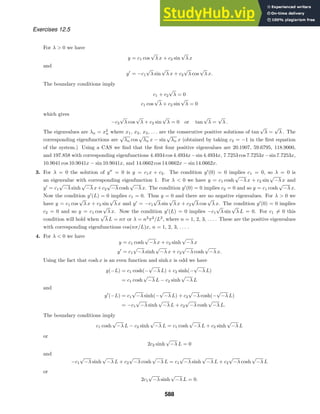

![Exercises 12.5
6. The eigenfunctions are sin
√
λn x where tan
√
λn = −λn. Thus
sin λn x2
=
1
0
sin2
λn x dx =
1
2
1
0
1 − cos 2 λn x dx
=
1
2
x −
1
2
√
λn
sin 2 λn x
1
0
=
1
2
1 −
1
2
√
λn
sin 2 λn
=
1
2
1 −
1
2
√
λn
2 sin λn cos λn
=
1
2
1 −
1
√
λn
tan λn cos λn cos λn
=
1
2
1 −
1
√
λn
− λn cos2
λn
=
1
2
1 + cos2
λn .
7. (a) If λ ≤ 0 the initial conditions imply y = 0. For λ 0 the general solution of the Cauchy-Euler differential
equation is y = c1 cos(
√
λ ln x) + c2 sin(
√
λ ln x). The condition y(1) = 0 implies c1 = 0, so that y =
c2 sin(
√
λ ln x). The condition y(5) = 0 implies
√
λ ln 5 = nπ, n = 1, 2, 3, . . . . Thus, the eigenvalues are
n2
π2
/(ln 5)2
for n = 1, 2, 3, . . . , with corresponding eigenfunctions sin[(nπ/ ln 5) ln x].
(b) The self-adjoint form is
d
dx
[xy
] +
λ
x
y = 0.
(c) An orthogonality relation is
5
1
sin
mπ
ln 5
ln x sin
nπ
ln 5
ln x dx = 0.
8. (a) The roots of the auxiliary equation m2
+m+λ = 0 are 1
2 (−1±
√
1 − 4λ ). When λ = 0 the general solution
of the differential equation is c1 + c2e−x
. The initial conditions imply c1 + c2 = 0 and c1 + c2e−2
= 0. Since
the determinant of the coefficients is not 0, the only solution of this homogeneous system is c1 = c2 = 0, in
which case y = 0. Similarly, if 0 λ 1
4 , the general solution is
y = c1e
1
2 (−1+
√
1−4λ )x
+ c2e
1
2 (−1−
√
1−4λ )x
.
In this case the initial conditions again imply c1 = c2 = 0, and so y = 0. Now, for λ 1
4 , the general
solution of the differential equation is
y = c1e−x/2
cos
√
4λ − 1 x + c2e−x/2
sin
√
4λ − 1 x.
The condition y(0) = 0 implies c1 = 0 so y = c2e−x/2
sin
√
4λ − 1 x. From
y(2) = c2e−1
sin 2
√
4λ − 1 = 0
we see that the eigenvalues are determined by 2
√
4λ − 1 = nπ for n = 1, 2, 3, . . . . Thus, the eigenvalues
are n2
π2
/42
+ 1/4 for n = 1, 2, 3, . . . , with corresponding eigenfunctions e−x/2
sin
nπ
2
x.
(b) The self-adjoint form is
d
dx
[ex
y
] + λex
y = 0.
(c) An orthogonality relation is
2
0
ex
e−x/2
sin
mπ
2
x e−x/2
cos
nπ
2
x dx =
2
0
sin
mπ
2
x cos
nπ
2
x dx = 0.
590](https://image.slidesharecdn.com/advancedengineeringmathematicssolutionsmanual-230807162553-1916df96/85/Advanced-Engineering-Mathematics-Solutions-Manual-pdf-590-320.jpg)

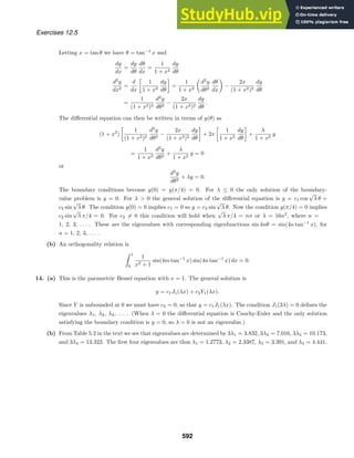
![Exercises 12.6
Exercises 12.6
1. Identifying b = 3, the first four eigenvalues are
λ1 =
3.832
3
≈ 1.277
λ2 =
7.016
3
≈ 2.339
λ3 =
10.173
3
= 3.391
λ4 =
13.323
3
≈ 4.441.
2. We first note from Case III in the text that 0 is an eigenvalue. Now, since J
0(2λ) = 0 is equivalent to J1(2λ) = 0,
the next three eigenvalues are
λ2 =
3.832
2
= 1.916
λ3 =
7.016
2
= 3.508
λ4 =
10.173
2
= 5.087.
3. The boundary condition indicates that we use (15) and (16) of Section 12.6. With b = 2 we obtain
ci =
2
4J2
1 (2λi)
2
0
xJ0(λix) dx
t = λix dt = λi dx
=
1
2J2
1 (2λi)
·
1
λ2
i
2λi
0
tJ0(t) dt
=
1
2λ2
i J2
1 (2λi)
2λi
0
d
dt
[tJ1(t)] dt [From (4) in the text]
=
1
2λ2
i J2
1 (2λi)
tJ1(t)
2λi
0
=
1
λiJ1(2λi)
.
Thus
f(x) =
∞
i=1
1
λiJ1(2λi)
J0(λix).
4. The boundary condition indicates that we use (19) and (20) of Section 12.6. With b = 2 we obtain
c1 =
2
4
2
0
x dx =
2
4
x2
2
2
0
= 1,
ci =
2
4J2
0 (2λi)
2
0
xJ0(λix) dx
t = λix dt = λi dx
=
1
2J2
0 (2λi)
·
1
λ2
i
2λi
0
tJ0(t) dt
593](https://image.slidesharecdn.com/advancedengineeringmathematicssolutionsmanual-230807162553-1916df96/85/Advanced-Engineering-Mathematics-Solutions-Manual-pdf-593-320.jpg)
![Exercises 12.6
=
1
2λ2
i J2
0 (2λi)
2λi
0
d
dt
[tJ1(t)] dt [From (4) in the text]
=
1
2λ2
i J2
0 (2λi)
tJ1(t)
2λi
0
=
J1(2λi)
λiJ2
0 (2λi)
.
Now since J
0(2λi) = 0 is equivalent to J1(2λi) = 0 we conclude ci = 0 for i = 2, 3, 4, . . . . Thus the expansion
of f on 0 x 2 consists of a series with one nontrivial term:
f(x) = c1 = 1.
5. The boundary condition indicates that we use (17) and (18) of Section 12.6. With b = 2 and h = 1 we obtain
ci =
2λ2
i
(4λ2
i + 1)J2
0 (2λi)
2
0
xJ0(λix) dx
t = λix dt = λi dx
=
2λ2
i
(4λ2
i + 1)J2
0 (2λi)
·
1
λ2
i
2λi
0
tJ0(t) dt
=
2
(4λ2
i + 1)J2
0 (2λi)
2λi
0
d
dt
[tJ1(t)] dt [From (4) in the text]
=
2
(4λ2
i + 1)J2
0 (2λi)
tJ1(t)
2λi
0
=
4λiJ1(2λi)
(4λ2
i + 1)J2
0 (2λi)
.
Thus
f(x) = 4
∞
i=1
λiJ1(2λi)
(4λ2
i + 1)J2
0 (2λi)
J0(λix).
6. Writing the boundary condition in the form
2J0(2λ) + 2λJ
0(2λ) = 0
we identify b = 2 and h = 2. Using (17) and (18) of Section 12.6 we obtain
ci =
2λ2
i
(4λ2
i + 4)J2
0 (2λi)
2
0
xJ0(λix) dx
t = λix dt = λi dx
=
λ2
i
2(λ2
i + 1)J2
0 (2λi)
·
1
λ2
i
2λi
0
tJ0(t) dt
=
1
2(λ2
i + 1)J2
0 (2λi)
2λi
0
d
dt
[tJ1(t)] dt [From (4) in the text]
=
1
2(λ2
i + 1)J2
0 (2λi)
tJ1(t)
2λi
0
=
λiJ1(2λi)
(λ2
i + 1)J2
0 (2λi)
.
594](https://image.slidesharecdn.com/advancedengineeringmathematicssolutionsmanual-230807162553-1916df96/85/Advanced-Engineering-Mathematics-Solutions-Manual-pdf-594-320.jpg)
![Exercises 12.6
Thus
f(x) =
∞
i=1
λiJ1(2λi)
(λ2
i + 1)J2
0 (2λi)
J0(λix).
7. The boundary condition indicates that we use (17) and (18) of Section 12.6. With n = 1, b = 4, and h = 3 we
obtain
ci =
2λ2
i
(16λ2
i − 1 + 9)J2
1 (4λi)
4
0
xJ1(λix)5x dx
t = λix dt = λi dx
=
5λ2
i
4(2λ2
i + 1)J2
1 (4λi)
·
1
λ3
i
4λi
0
t2
J1(t) dt
=
5
4λi(2λ2
i + 1)J2
1 (4λi)
4λi
0
d
dt
[t2
J2(t)] dt [From (4) in the text]
=
5
4λi(2λ2
i + 1)J2
1 (4λi)
t2
J2(t)
4λi
0
=
20λiJ2(4λi)
(2λ2
i + 1)J2
1 (4λi)
.
Thus
f(x) = 20
∞
i=1
λiJ2(4λi)
(2λ2
i + 1)J2
1 (4λi)
J1(λix).
8. The boundary condition indicates that we use (15) and (16) of Section 12.6. With n = 2 and b = 1 we obtain
c1 =
2
J2
3 (λi)
1
0
xJ2(λix)x2
dx
t = λix dt = λi dx
=
2
J2
3 (λi)
·
1
λ4
i
λi
0
t3
J2(t) dt
=
2
λ4
i J2
3 (λi)
λi
0
d
dt
[t3
J3(t)] dt [From (4) in the text]
=
2
λ4
i J2
3 (λi)
t3
J3(t)
λi
0
=
2
λiJ3(λi)
.
Thus
f(x) = 2
∞
i=1
1
λiJ3(λi)
J2(λix).
9. The boundary condition indicates that we use (19) and (20) of Section 12.6. With b = 3 we obtain
c1 =
2
9
3
0
xx2
dx =
2
9
x4
4
3
0
=
9
2
,
ci =
2
9J2
0 (3λi)
3
0
xJ0(λix)x2
dx
t = λix dt = λi dx
595](https://image.slidesharecdn.com/advancedengineeringmathematicssolutionsmanual-230807162553-1916df96/85/Advanced-Engineering-Mathematics-Solutions-Manual-pdf-595-320.jpg)
![Exercises 12.6
=
2
9J2
0 (3λi)
·
1
λ4
i
3λi
0
t3
J0(t) dt
=
2
9λ4
i J2
0 (3λi)
3λi
0
t2 d
dt
[tJ1(t)] dt
u = t2
dv = d
dt [tJ1(t)] dt
du = 2t dt v = tJ1(t)
=
2
9λ4
i J2
0 (3λi)
t3
J1(t)
3λi
0
−2
3λi
0
t2
J1(t) dt
With n = 0 in equation (5) in Section 12.6 in the text we have J
0(x) = −J1(x), so the boundary condition
J
0(3λi) = 0 implies J1(3λi) = 0. Then
ci =
2
9λ4
i J2
0 (3λi)
−2
3λi
0
d
dt
t2
J2(t)
dt
=
2
9λ4
i J2
0 (3λi)
−2t2
J2(t)
3λi
0
=
2
9λ4
i J2
0 (3λi)
−18λ2
i J2(3λi)
=
−4J2(3λi)
λ2
i J2
0 (3λi)
.
Thus
f(x) =
9
2
− 4
∞
i=1
J2(3λi)
λ2
i J2
0 (3λi)
J0(λix).
10. The boundary condition indicates that we use (15) and (16) of Section 12.6. With b = 1 it follows that
ci =
2
J2
1 (λi)
1
0
x
1 − x2
J0(λix) dx
=
2
J2
1 (λi)
1
0
xJ0(λix) dx −
1
0
x3
J0(λix) dx
t = λix dt = λi dx
=
2
J2
1 (λi)
1
λ2
i
λi
0
tJ0(t) dt −
1
λ4
i
λi
0
t3
J0(t) dt
=
2
J2
1 (λi)
1
λ2
i
λi
0
d
dt
(tJ1(t)) dt −
1
λ4
i
λi
0
t2 d
dt
[tJ1(t)] dt
u = t2
dv = d
dt [tJ1(t)] dt
du = 2t dt v = tJ1(t)
=
2
J2
1 (λi)
1
λ2
i
tJ1(t)
λi
0
−
1
λ4
i
t3
J1(t)
λi
0
− 2
λi
0
t2
J1(t) dt
=
2
J2
1 (λi)
J1(λi)
λi
−
J1(λi)
λi
+
2
λ4
i
λi
0
d
dt
t2
J2(t)
dt
=
2
J2
1 (λi)
2
λ4
i
t2
J2(t)
λi
0
=
4J2(λi)
λ2
i J2
1 (λi)
.
596](https://image.slidesharecdn.com/advancedengineeringmathematicssolutionsmanual-230807162553-1916df96/85/Advanced-Engineering-Mathematics-Solutions-Manual-pdf-596-320.jpg)
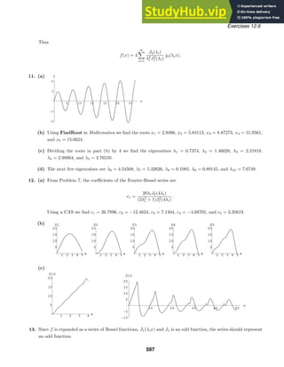


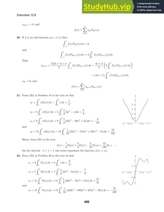
![Chapter 12 Review Exercises
Hence, from (27) in the text,
f(x) =
3
2
P1(x) −
7
8
P3(x) +
11
16
P5(x) −
75
128
P7(x) + · · · .
On the interval −1 x 1 this series represents the odd function
f(x) =
−1, −1 x 0
1, 0 x 1.
Chapter 12 Review Exercises
1. True, since
π
−π
(x2
− 1)x5
dx = 0
2. Even, since if f and g are odd then h(−x) = f(−x)g(−x) = −f(x)[−g(x)] = f(x)g(x) = h(x)
3. Cosine, since f is even
4. True
5. False; the Sturm-Liouville problem,
d
dx
[r(x)y
] + λp(x)y = 0, y
(a) = 0, y
(b) = 0,
on the interval [a, b], has eigenvalue λ = 0.
6. 3/2, the average of 3 and 0
7. The Fourier series will converge to 1, the cosine series to 1, and the sine series to 0 at x = 0. Respectively, this
is because the rule (x2
+ 1) defining f(x) determines a continuous function on (−3, 3), the even extension of f
to (−3, 0) is continuous at 0, and the odd extension of f to (−3, 0) approaches −1 as x approaches 0 from the
left.
8. cos 5x, since the general solution is y = c1 cos
√
λ x + c2 sin
√
λ x and y
(0) = 0 implies c2 = 0.
9. Since the coefficient of y in the differential equation is n2
, the weight function is the integrating factor
1
a(x)
e
(b/a)dx
=
1
1 − x2
e
− x
1−x2 dx
=
1
1 − x2
e
1
2 ln(1−x2
)
=
√
1 − x2
1 − x2
=
1
√
1 − x2
on the interval [−1, 1]. The orthogonality relation is
1
−1
1
√
1 − x2
Tm(x)Tn(x) dx = 0, m = n.
10. Since Pn(x) is orthogonal to P0(x) = 1 for n 0,
1
−1
Pn(x) dx =
1
−1
P0(x)Pn(x) dx = 0.
11. We know from a half-angle formula in trigonometry that cos2
x = 1
2 + 1
2 cos 2x, which is a cosine series.
12. (a) For m = n
L
0
sin
(2n + 1)π
2L
x sin
(2m + 1)π
2L
x dx =
1
2
L
0
cos
n − m
L
πx − cos
n + m + π
L
πx
dx = 0.
(b) From
L
0
sin2 (2n + 1)π
2L
x dx =
L
0
1
2
−
1
2
cos
(2n + 1)π
2L
x
dx =
L
2
601](https://image.slidesharecdn.com/advancedengineeringmathematicssolutionsmanual-230807162553-1916df96/85/Advanced-Engineering-Mathematics-Solutions-Manual-pdf-601-320.jpg)
![Chapter 12 Review Exercises
we see that
sin
(2n + 1)π
2L
x =
L
2
.
13. Since
A0 =
0
−1
(−2x) dx = 1,
An =
0
−1
(−2x) cos nπx dx =
2
n2π2
[(−1)n
− 1],
and
Bn =
0
−1
(−2x) sin nπx dx =
4
nπ
(−1)n
for n = 1, 2, 3, . . . we have
f(x) =
1
2
+
∞
n=1
2
n2π2
[(−1)n
− 1] cos nπx +
4
nπ
(−1)n
sin nπx
.
14. Since
A0 =
1
−1
(2x2
− 1) dx = −
2
3
,
An =
1
−1
(2x2
− 1) cos nπx dx =
8
n2π2
(−1)n
,
and
Bn =
1
−1
(2x2
− 1) sin nπx dx = 0
for n = 1, 2, 3, . . . we have
f(x) = −
1
3
+
∞
n=1
8
n2π2
(−1)n
cos nπx.
15. Since
A0 = 2
1
0
e−x
dx
and
An = 2
1
−1
e−x
cos nπx dx =
2
1 + n2π2
[(1 − (−1)n
e−1
]
for n = 1, 2, 3, . . . we have
f(x) = 1 − e−1
+ 2
∞
n=1
1 − (−1)n
e−1
1 + n2π2
cos nπx.
Since
Bn = 2
1
0
e−x
sin nπx dx =
2nπ
1 + n2π2
[(1 − (−1)n
e−1
]
for n = 1, 2, 3, . . . we have
f(x) =
∞
n=1
2nπ
1 + n2π2
[(1 − (−1)n
e−1
] sin nπx.
602](https://image.slidesharecdn.com/advancedengineeringmathematicssolutionsmanual-230807162553-1916df96/85/Advanced-Engineering-Mathematics-Solutions-Manual-pdf-602-320.jpg)
![-1 -0.5 0.5 1 x
0.5
1
1.5
2
fHxL
-1 -0.5 0.5 1 x
-1
-0.5
0.5
1
y
-1 -0.5 0.5 1 x
-1
-0.5
0.5
1
y
-1 -0.5 0.5 1 x
-1
-0.5
0.5
1
y
Chapter 12 Review Exercises
16.
f(x) = |x| − 1 f(x) = 2x2
− 1 f(x) = e−|x|
f(x) =
e−x
, 0 x 1
0, x = 0
−ex
, −1 x 0
17. For λ 0 a general solution of the given differential equation is
y = c1 cos(3
√
λ ln x) + c2 sin(3
√
λ ln x)
and
y
= −
3c1
√
λ
x
sin(3
√
λ ln x) +
3c2
√
λ
x
cos(3
√
λ ln x).
Since ln 1 = 0, the boundary condition y
(1) = 0 implies c2 = 0. Therefore
y = c1 cos(3
√
λ ln x).
Using ln e = 1 we find that y(e) = 0 implies c1 cos 3
√
λ = 0 or 3
√
λ =
2n − 1
2
π , for n = 1, 2, 3, . . . . The
eigenvalues are λ = (2n − 1)2
π2
/36 with corresponding eigenfunctions cos
2n − 1
2
π ln x
for n = 1, 2, 3, . . . .
18. To obtain the self-adjoint form of the differential equation in Problem 17 we note that an integrating factor is
(1/x2
)e
dx/x
= 1/x. Thus the weight function is 9/x and an orthogonality relation is
e
1
9
x
cos
2n − 1
2
π ln x
cos
2m − 1
2
π ln x
dx = 0, m = n.
19. The boundary condition indicates that we use (15) and (16) of Section 12.6. With b = 4 we obtain
ci =
2
16J2
1 (4λi)
4
0
xJ0(λix)f(x) dx
=
1
8J2
1 (4λi)
2
0
xJ0(λix) dx
t = λix dt = λi dx
=
1
8J2
1 (4λi)
·
1
λ2
i
2λi
0
tJ0(t) dt
=
1
8J2
1 (4λi)
2λi
0
d
dt
[tJ1(t)] dt [From (4) in 12.6 in the text]
=
1
8J2
1 (4λi)
tJ1(t)
2λi
0
=
J1(2λi)
4λiJ2
1 (4λi)
.
Thus
f(x) =
1
4
∞
i=1
J1(2λi)
λiJ2
1 (4λi)
J0(λix).
20. Since f(x) = x4
is a polynomial in x, an expansion of f in polynomials in x must terminate with the term
having the same degree as f. Using the fact that x4
P1(x) and x4
P3(x) are odd functions, we see immediately
603](https://image.slidesharecdn.com/advancedengineeringmathematicssolutionsmanual-230807162553-1916df96/85/Advanced-Engineering-Mathematics-Solutions-Manual-pdf-603-320.jpg)

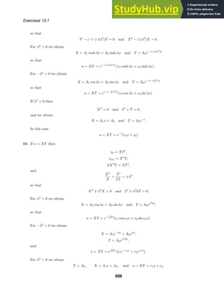
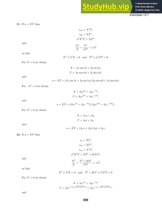
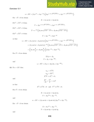
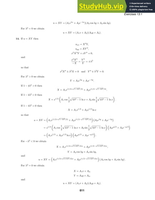
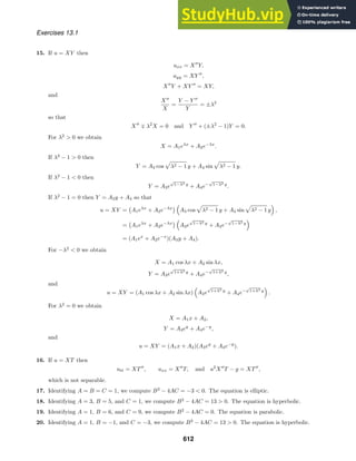
![Exercises 13.1
21. Identifying A = 1, B = −9, and C = 0, we compute B2
− 4AC = 81 0. The equation is hyperbolic.
22. Identifying A = 0, B = 1, and C = 0, we compute B2
− 4AC = 1 0. The equation is hyperbolic.
23. Identifying A = 1, B = 2, and C = 1, we compute B2
− 4AC = 0. The equation is parabolic.
24. Identifying A = 1, B = 0, and C = 1, we compute B2
− 4AC = −4 0. The equation is elliptic.
25. Identifying A = a2
, B = 0, and C = −1, we compute B2
− 4AC = 4a2
0. The equation is hyperbolic.
26. Identifying A = k 0, B = 0, and C = 0, we compute B2
− 4AC = −4k 0. The equation is elliptic.
27. If u = RT then
ur = R
T,
urr = R
T,
ut = RT
,
RT
= k
R
T +
1
r
R
T
,
and
r2
R
+ rR
r2R
=
T
kT
= ±λ2
.
If we use −λ2
0 then
r2
R
+ rR
+ λ2
r2
R = 0 and T
∓ λ2
kT = 0
so that
R = A2J0(λr) + A3Y0(λr),
T = A1e−kλ2
t
,
and
u = RT = e−kλ2
t
[c1J0(λr) + c2Y0(λr)]
28. If u = RΘ then
ur = R
Θ,
urr = R
Θ,
ut = RΘ
,
utt = RΘ
,
R
Θ +
1
r
R
Θ +
1
r2
RΘ
= 0,
and
r2
R
+ rR
R
= −
Θ
Θ
= λ2
.
Then
r2
R
+ rR
− λ2
R = 0 and Θ
+ λ2
Θ = 0
so that
R = c3rλ
+ c4r−λ
Θθ = c1 cos λθ + c2 sin λθ,
and
u = RΘ = (c1 cos λθ + c2 sin λθ)(c3rλ
+ c4r−λ
).
613](https://image.slidesharecdn.com/advancedengineeringmathematicssolutionsmanual-230807162553-1916df96/85/Advanced-Engineering-Mathematics-Solutions-Manual-pdf-613-320.jpg)
![Exercises 13.3
Imposing
u(x, 0) =
∞
n=1
An sin
nπ
L
x
gives
An =
2
L
L/2
0
sin
nπ
L
x dx =
2
nπ
1 − cos
nπ
2
for n = 1, 2, 3, . . . so that
u(x, t) =
2
π
∞
n=1
1 − cos nπ
2
n
e− kn2π2
L2 t
sin
nπ
L
x.
2. Using u = XT and −λ2
as a separation constant leads to
X
+ λ2
X = 0,
X(0) = 0,
X(L) = 0,
and
T
+ kλ2
T = 0.
Then
X = c1 sin
nπ
L
x and T = c2e− kn2π2
L2 t
for n = 1, 2, 3, . . . so that
u =
∞
n=1
Ane− kn2π2
L2 t
sin
nπ
L
x.
Imposing
u(x, 0) =
∞
n=1
An sin
nπ
L
x
gives
An =
2
L
L
0
x(L − x) sin
nπ
L
x dx =
4L2
n3π3
[1 − (−1)n
]
for n = 1, 2, 3, . . . so that
u(x, t) =
4L2
π3
∞
n=1
1 − (−1)n
n3
e− kn2π2
L2 t
sin
nπ
L
x.
3. Using u = XT and −λ2
as a separation constant leads to
X
+ λ2
X = 0,
X
(0) = 0,
X
(L) = 0,
and
T
+ kλ2
T = 0.
Then
X = c1 cos
nπ
L
x and T = c2e− kn2π2
L2 t
for n = 0, 1, 2, . . . so that
u =
∞
n=0
Ane− kn2π2
L2 t
cos
nπ
L
x.
616](https://image.slidesharecdn.com/advancedengineeringmathematicssolutionsmanual-230807162553-1916df96/85/Advanced-Engineering-Mathematics-Solutions-Manual-pdf-616-320.jpg)
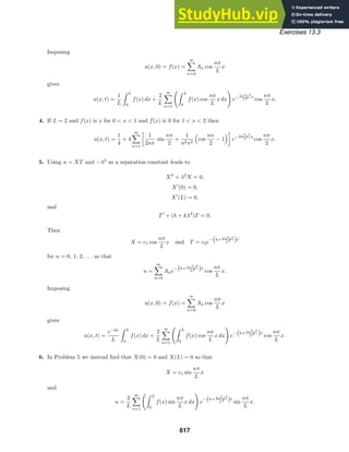


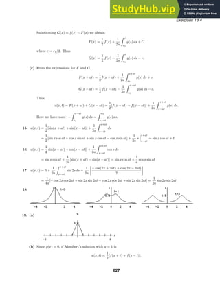
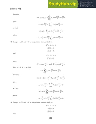

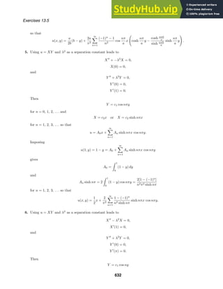


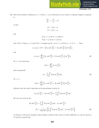
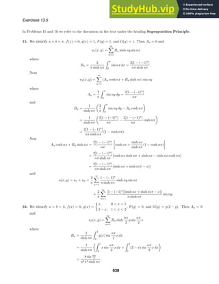

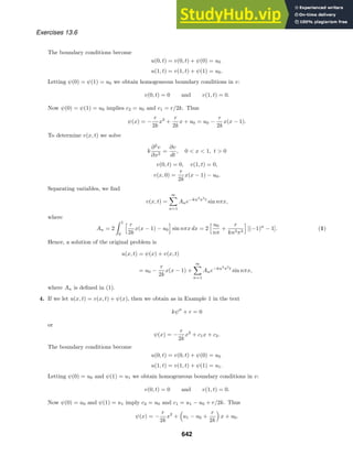

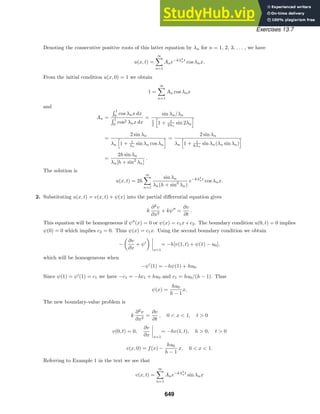
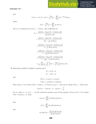
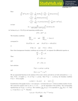
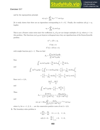


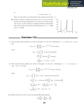
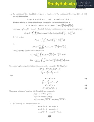


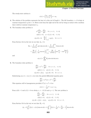


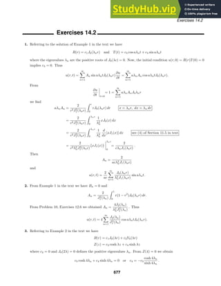


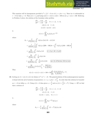

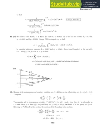
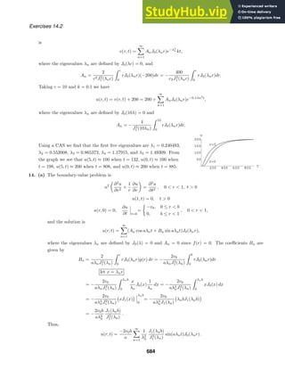
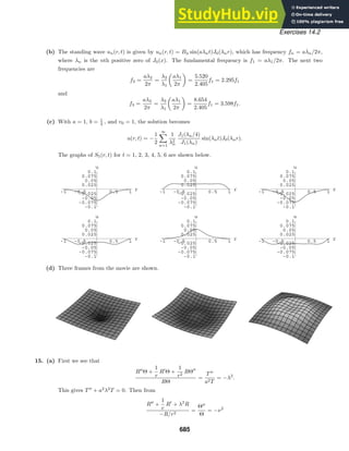

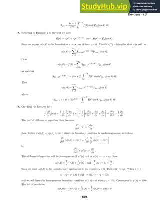

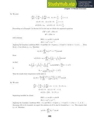

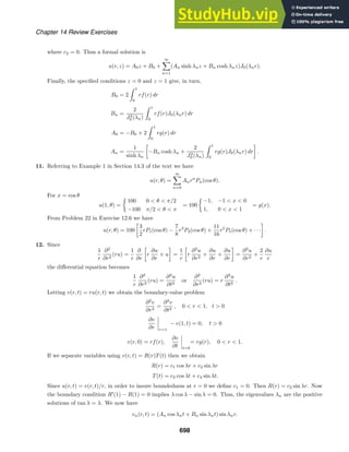
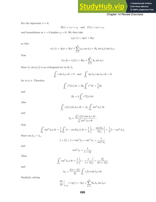

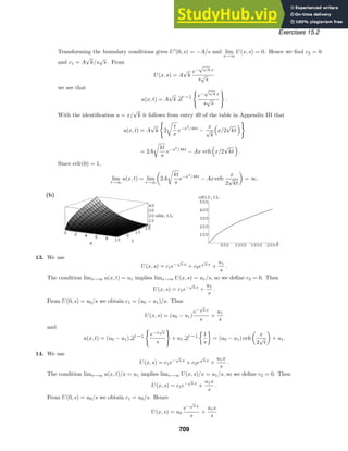


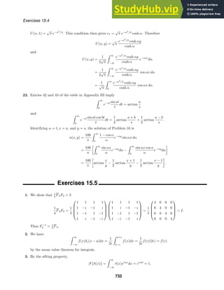

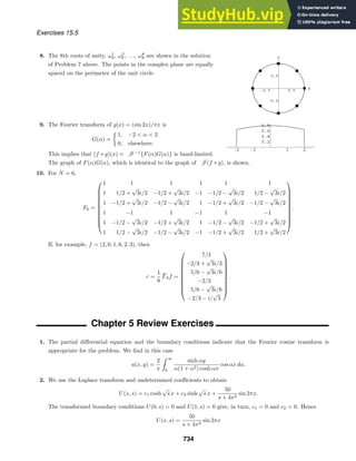

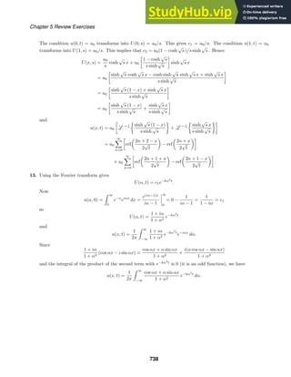
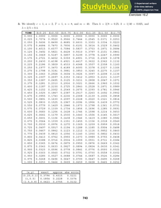
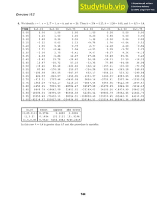
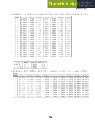
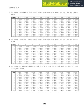
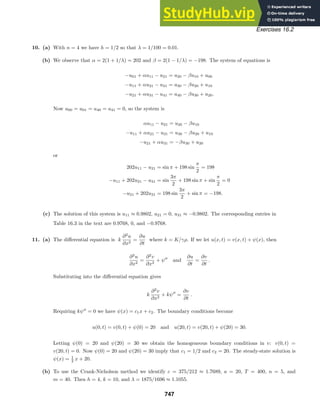
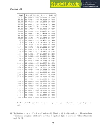
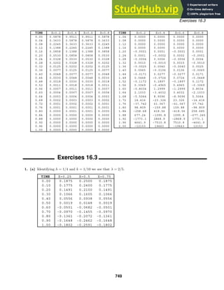
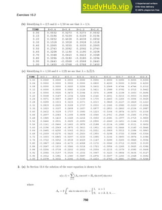


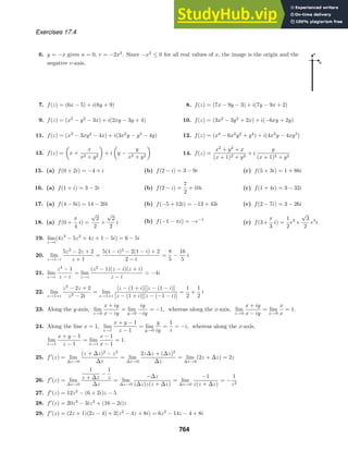


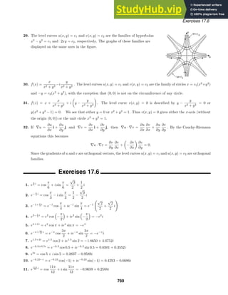

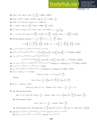
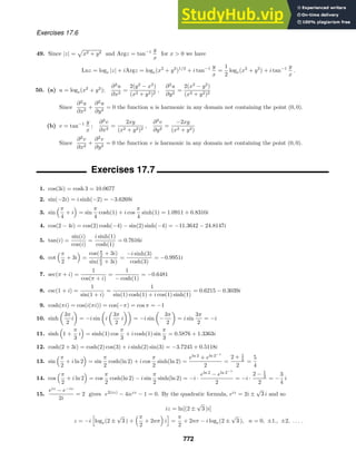
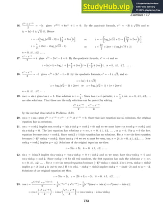


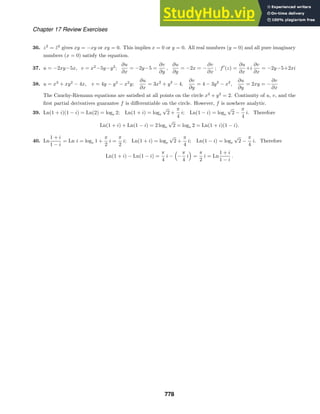


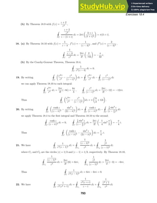

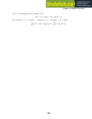


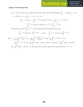

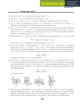
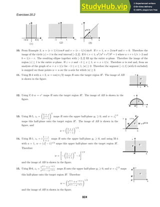
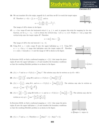
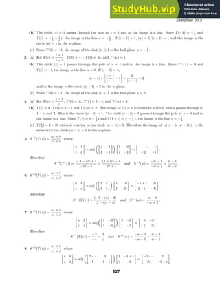
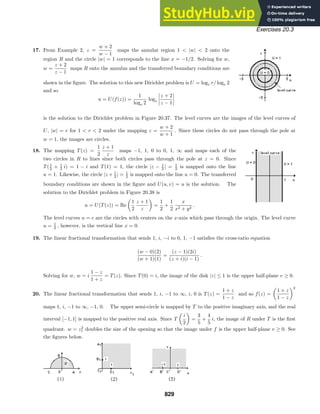
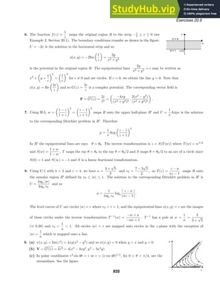
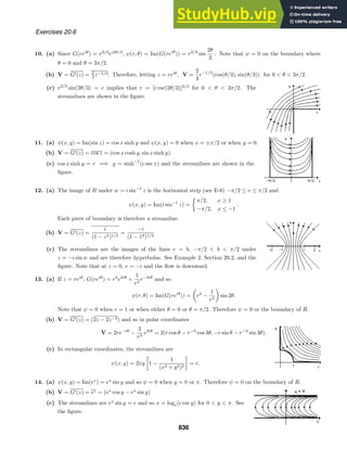
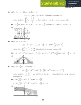
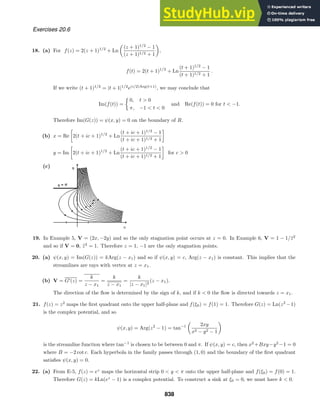
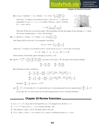
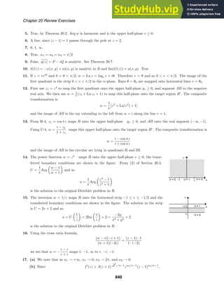
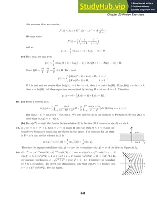

This document contains 27 multi-part exercises involving differential equations. The exercises cover topics such as determining whether differential equations are linear or nonlinear, solving differential equations, and classifying differential equations by order.