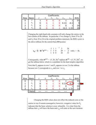
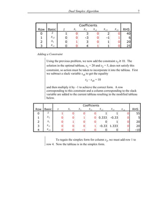
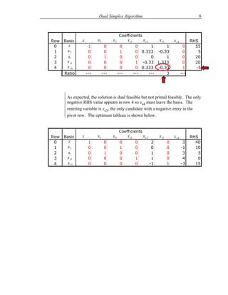
Operations Research Models and Methods
                                                      Paul A. Jensen and Jonathan F. Bard

LP Methods.S1
Dual Simplex Algorithm
In the tableau implementation of the primal simplex algorithm, the right-hand-side
column is always nonnegative so the basic solution is feasible at every iteration. For
purposes of this section, we will say that the basis for the tableau is primal feasible if all
elements of the right-hand side are nonnegative. Alternatively, when some of the
elements are negative, we say that the basis is primal infeasible. Up to this point we have
always been concerned with primal feasible bases.
        For the primal simplex algorithm, some elements in row 0 will be negative until
the final iteration when the optimality conditions are satisfied. In the event that all
elements of row 0 are nonnegative, we say that the associated basis is dual feasible.
Alternatively, if some of the elements of row 0 are negative, we have a dual infeasible
basis.
        As described, the primal simplex method works with primal feasible, but dual
infeasible (nonoptimal) bases. At the final (optimal) solution, the basis is both primal and
dual feasible. Throughout the process we maintain primal feasibility and drive toward
dual feasibility.
        In this section, a variant of the primal approach, known as the dual simplex
method, is considered that works in just the opposite fashion. Until the final iteration,
each basis examined is primal infeasible (some negative values on the right-hand side)
and dual feasible (all elements in row 0 are nonnegative). At the final (optimal) iteration
the solution will be both primal and dual feasible. Throughout the process we maintain
dual feasibility and drive toward primal feasibility. For a given problem, both the primal
and dual simplex algorithms will terminate at the same solution but arrive there from
different directions.
         The dual simplex algorithm is most suited for problems for which an initial dual
feasible solution is easily available. It is particularly useful for reoptimizing a problem
after a constraint has been added or some parameters have been changed so that the
previously optimal basis is no longer feasible.
        We will have much more to say about duality and the relationship between primal
and dual solutions in Chapter 5; however, in this section, we are principally concerned
with the mechanics of implementing the dual simplex method in the tableau format. We
will see that the dual simplex algorithm is very similar to the primal simplex algorithm.

Algorithm

               With reference to the tableau, the algorithm must begin with a basic
               solution that is dual feasible so all the elements of row 0 must be
               nonnnegative. The iterative step of the primal simplex algorithm first
               selects a variable to enter the basis and then finds the variable that must
               leave so that primal feasibility is maintained. The dual simplex method
               does the opposite; it first selects a variable to leave the basis and then finds
Dual Simplex Algorithm                                     2


        the variable that must enter the basis to maintain dual feasibility. This is
        the principal difference between the two methods. The algorithm below
        assumes a basic solution is described by a tableau.

Step 1 (Initialization)

        Start with a dual feasible basis and let k = 1. Create a tableau for this basis
        in the simplex form. If the right-hand side entries are all nonnegative, the
        solution is primal feasible, so stop with the optimal solution.

Step 2 (Iteration k)

           a.   Select the leaving variable. Find a row, call it r, with a negative
                                                -
                right-hand-side constant; i.e., br < 0. Let row r be the pivot row
                and let the leaving variable be xB(r). A common rule for choosing r
                is to select the most negative RHS value; i.e.,

                                   -        -
                                   br = min{bi : i = 1, … ,m}.

           b.   Determine the entering variable. For each negative coefficient in
                the pivot row, compute the negative of the ratio between the
                reduced cost in row 0 and the structural coefficient in row r. If
                                                  -
                there is no negative coefficient, a < 0, stop; there is no feasible
                                                   rj
                solution.
                        Let the column with the minimum ratio, designated by the
                index s, be the pivot column; let xs is the entering variable. The
                pivot column is determined by the following ratio test.
                              -
                            – cs       –c
                                       -j -                      
                                                                  
                                = min     : arj < 0, j = 1, … ,n 
                            -
                            ars       a-
                                       rj                        
                                                                  


           c.   Change the basis. Replace xB(r) by xs in the basis. Create a new
                tableau by performing the following operations (these are the same
                as for the primal simplex algorithm).

                     -
                Let ai be the vector of the ith row of the current tableau, and let
                - new                                         -
                ai be the ith row in the new tableau. Let bi be the RHS for row i
                                                 - new
                in the current tableau, and let bi be the RHS of the new tableau.
                     -
                Let a be the element in the ith row of the pivot column s.
                       is
Dual Simplex Algorithm                                     3


                     The pivot row in the new tableau is
                                  - new - -         - new - -
                                  ar = ar / ars and br = br /ars.
                     The other rows in the new tableau are


                                      ai = – ais × ar  + ai and
                                      - new   -     - new   -
                                                         

                          - new  -     - new -
                          bi = – ais × br  + bi for i = 0, 1 , … ,m, i ≠ r


                  (These operations have the effect of pricing out the pivot column. Its
                  replacement will have a single 1 in row r and a zero in all other rows
                  as required by the simplex form.)

     Step 3 (Feasibility test)

             If all entries on the right-hand side are nonnegative the solution is primal
             feasible, so stop with the optimal solution. Otherwise, put k ← k +1 and
             return to Step 2.

Examples

     An Easy Dual Feasible Starting Solution

             The simplest situation arises when there is an obvious dual feasible basis
             that can be used to initialize the algorithm. Consider the following
             problem.


                         Maximize z = –5x1 – 35x2– 20x3
                         subject to         x1    – x2     – x3 ≤ – 2
                                           –x1    –3x2            ≤ –3
                                         x1 ≥ 0, x2 ≥ 0, x3 ≥ 0


             Step 1: Adding slack variables x4 and x5, leads to the first tableau which is
             primal infeasible but dual feasible.
Dual Simplex Algorithm                                        4


                                    Coefficients
Row   Basic    z         x1          x2        x3         x4         x5         RHS
 0     z            1          5          35        20          0          0       0
 1     x4           0          1          -1        -1          1          0      -2
 2     x5           0         -1          -3         0          0          1      -3


      Iteration 1: Row 2 is selected as the pivot row so x5 leaves the basis. The
      ratio test indicates that x1 is to enter the basis. The tableau shows the ratio
      calculations.

                                    Coefficients
Row   Basic    z         x1          x2        x3         x4         x5         RHS
 0     z            1          5    35              20          0          0       0
 1     x4           0          1    -1              -1          1          0      -2
 2     x5           0         -1    -3               0          0          1      -3
      Ratio        ---         5 11.67              ---        ---        ---


      After the pricing out operations to obtain the simplex form for x1 we get
      the following tableau. The feasibility test at Step 3 fails because the basis
      is not yet primal feasible so we return to Step 2. We show the row and
      column selection steps for the next iteration.


                                    Coefficients
Row   Basic    z         x1          x2        x3         x4         x5         RHS
 0     z            1          0          20        20          0          5     -15
 1     x4           0          0          -4        -1          1          1      -5
 2     x1           0          1           3         0          0         -1       3
      Ratio        ---        ---          5        20         ---        ---


      Iteration 2: Row 1 is selected as the pivot row so x4 leaves the basis and x2
      enters. This leads to the tableau below that still has a negative RHS value
      so we return to Step 2.
Dual Simplex Algorithm                                      5


                                     Coefficients
Row   Basic     z         x1          x2         x3          x4       x5      RHS
 0     z             1          0           0       15           5       10     -40
 1     x2            0          0           1     0.25       -0.25    -0.25    1.25
 2      x1           0          1           0    -0.75        0.75    -0.25   -0.75
      Ratio         ---        ---         ---      20          ---      40


       Iteration 3: Selecting row 2 as the pivot row, x1 leaves the basis and x3
       enters. The updated tableau given below is both primal and dual feasible
       indicating that the optimal solution has been obtained. The algorithm
       terminates.


                                     Coefficients
Row   Basic     z         x1          x2         x3          x4       x5      RHS
 0     z             1    20                0            0        20     5     -55
 1     x2            0 0.333                1            0         0 -0.33       1
 2      x3           0 -1.33                0            1        -1 0.333       1


Restarting after Changing the Right-Hand-Side Constants

       A primary use of the dual simplex algorithm is to reoptimize a problem
       after it has been solved and one or more of the RHS constants is changed.
       This is illustrated with the following problem. The optimal tableau is also
       shown with xs1, xs2, and xs3 as slacks.
                    Maximize z =        2x1      + 3x2
                    subject to          –x1       + x2 ≤ 5
                                           x1    + 3x2 ≤ 35
                                           x1            ≤ 20
                                           x1 ≥ 0, x2 ≥ 0
Dual Simplex Algorithm                                     6


                                     Coefficients
Row    Basic        z          x1       x2    x s1        xs2      x s3   RHS
 0        z             1        0       0           0       1       1      55
 1        x2            0        0       1           0    0.33    -0.3       5
 2        x1            0        1       0           0       0       1      20
 3        x s1          0        0       0           1    -0.3    1.33      20


      Changing the right-hand-side constants will only change the entries in the
      last column of the tableau. In particular, if we change b2 from 35 to 20
      and b3 from 20 to 26 in the original problem statement, the RHS vector in
      the above tableau for the current basis B becomes


                                                   –1
                                  –1 1 1              5    26
                  -     –1bnew =  1 3 0                     
             xB = b = B                               20 = –2 with z = 46.
                                  1 0 0               26   33


      Consequently, when bnew = (5, 20, 26)T replaces bold = (5, 35, 20)T, we
      get the tableau below which is a candidate for the dual simplex algorithm.
                 -                       -
      Note that b2 appears in row 1 and b1 appears in row 2 in the tableau
      because row 2 corresponds to x1 and row 1 to x2.


                                     Coefficients
Row    Basic        z          x1       x2    x s1        xs2      x s3   RHS
 0       z           1          0        0          0    1    1             55
 1       x2          0          0        1          0 0.33 -0.3             -2
 2       x1          0          1        0          0    0    1             26
 3       x s1        0          0        0          1 -0.3 1.33             33
       Ratio        ---        ---      ---        ---  ---   3


              Changing the RHS values does not effect the reduced costs so the
                                                                               -
      entries in row 0 remain nonnegative; however, a negative value for b2
      indicates that the basic solution is now infeasible. It is clear from the
      tableau that x2 will leave the basis and xs3 will enter at the next iteration.
Dual Simplex Algorithm                                                        7


                                                  Coefficients
 Row    Basic                z            x1            x2          x s1          xs2           x s3    RHS
  0           z                  1            0          3              0            2             0      40
  1           x s3               0            0         -3              0           -1             1       6
  2           x1                 0            1          3              0            1             0      20
  3           x s1               0            0          4              1            1             0      25

Adding a Constraint

       Using the previous problem, we now add the constraint x2 ≥ 10. The
       solution in the optimal tableau, x1 = 20 and x2 = 5, does not satisfy this
       constraint, so action must be taken to incorporate it into the tableau. First
       we subtract a slack variable xs4 to get the equality
                                                        x2 – xs4 = 10

       and then multiply it by –1 to achieve the correct form. A row
       corresponding to this constraint and a column corresponding to the slack
       variable are added to the current tableau resulting in the modified tableau
       below.

                                                       Coefficients
Row   Basic          z               x1           x2         x s1           xs2          x s3          xs4       RHS
 0     z                 1                0             0            0     1     1                           0     55
 1     x2                0                0             1            0 0.333 -0.33                           0      5
 2     x1                0                1             0            0     0     1                           0     20
 3     x s1              0                0             0            1 -0.33 1.333                           0     20
 4     xs4               0                0            -1            0     0     0                           1    -10


              To regain the simplex form for column x2, we must add row 1 to
       row 4. Now the tableau is in the simplex form.
Dual Simplex Algorithm                                                8


                                         Coefficients
Row   Basic    z         x1         x2         x s1       xs2        x s3       xs4         RHS
 0     z            1          0          0            0     1     1                   0      55
 1     x2           0          0          1            0 0.333 -0.33                   0       5
 2     x1           0          1          0            0     0     1                   0      20
 3     x s1         0          0          0            1 -0.33 1.333                   0      20
 4     xs4          0          0          0            0 0.333 -0.33                   1      -5
      Ratio        ---        ---        ---          ---   ---    3                  ---


       As expected, the solution is dual feasible but not primal feasible. The only
       negative RHS value appears in row 4 so xs4 must leave the basis. The
       entering variable is xs3, the only candidate with a negative entry in the
       pivot row. The optimum tableau is shown below.


                                         Coefficients
Row   Basic    z         x1         x2         x s1       xs2        x s3       xs4         RHS
 0     z            1          0          0           0          2          0          3      40
 1     x2           0          0          1           0          0          0         -1      10
 2     x1           0          1          0           0          1          0          3       5
 3     x s1         0          0          0           1          1          0          4       0
 4     x s3         0          0          0           0         -1          1         -3      15

S1 Dualsimplex

  • 1.
    Operations Research Modelsand Methods Paul A. Jensen and Jonathan F. Bard LP Methods.S1 Dual Simplex Algorithm In the tableau implementation of the primal simplex algorithm, the right-hand-side column is always nonnegative so the basic solution is feasible at every iteration. For purposes of this section, we will say that the basis for the tableau is primal feasible if all elements of the right-hand side are nonnegative. Alternatively, when some of the elements are negative, we say that the basis is primal infeasible. Up to this point we have always been concerned with primal feasible bases. For the primal simplex algorithm, some elements in row 0 will be negative until the final iteration when the optimality conditions are satisfied. In the event that all elements of row 0 are nonnegative, we say that the associated basis is dual feasible. Alternatively, if some of the elements of row 0 are negative, we have a dual infeasible basis. As described, the primal simplex method works with primal feasible, but dual infeasible (nonoptimal) bases. At the final (optimal) solution, the basis is both primal and dual feasible. Throughout the process we maintain primal feasibility and drive toward dual feasibility. In this section, a variant of the primal approach, known as the dual simplex method, is considered that works in just the opposite fashion. Until the final iteration, each basis examined is primal infeasible (some negative values on the right-hand side) and dual feasible (all elements in row 0 are nonnegative). At the final (optimal) iteration the solution will be both primal and dual feasible. Throughout the process we maintain dual feasibility and drive toward primal feasibility. For a given problem, both the primal and dual simplex algorithms will terminate at the same solution but arrive there from different directions. The dual simplex algorithm is most suited for problems for which an initial dual feasible solution is easily available. It is particularly useful for reoptimizing a problem after a constraint has been added or some parameters have been changed so that the previously optimal basis is no longer feasible. We will have much more to say about duality and the relationship between primal and dual solutions in Chapter 5; however, in this section, we are principally concerned with the mechanics of implementing the dual simplex method in the tableau format. We will see that the dual simplex algorithm is very similar to the primal simplex algorithm. Algorithm With reference to the tableau, the algorithm must begin with a basic solution that is dual feasible so all the elements of row 0 must be nonnnegative. The iterative step of the primal simplex algorithm first selects a variable to enter the basis and then finds the variable that must leave so that primal feasibility is maintained. The dual simplex method does the opposite; it first selects a variable to leave the basis and then finds
  • 2.
    Dual Simplex Algorithm 2 the variable that must enter the basis to maintain dual feasibility. This is the principal difference between the two methods. The algorithm below assumes a basic solution is described by a tableau. Step 1 (Initialization) Start with a dual feasible basis and let k = 1. Create a tableau for this basis in the simplex form. If the right-hand side entries are all nonnegative, the solution is primal feasible, so stop with the optimal solution. Step 2 (Iteration k) a. Select the leaving variable. Find a row, call it r, with a negative - right-hand-side constant; i.e., br < 0. Let row r be the pivot row and let the leaving variable be xB(r). A common rule for choosing r is to select the most negative RHS value; i.e., - - br = min{bi : i = 1, … ,m}. b. Determine the entering variable. For each negative coefficient in the pivot row, compute the negative of the ratio between the reduced cost in row 0 and the structural coefficient in row r. If - there is no negative coefficient, a < 0, stop; there is no feasible rj solution. Let the column with the minimum ratio, designated by the index s, be the pivot column; let xs is the entering variable. The pivot column is determined by the following ratio test. - – cs  –c  -j -   = min  : arj < 0, j = 1, … ,n  - ars a-  rj   c. Change the basis. Replace xB(r) by xs in the basis. Create a new tableau by performing the following operations (these are the same as for the primal simplex algorithm). - Let ai be the vector of the ith row of the current tableau, and let - new - ai be the ith row in the new tableau. Let bi be the RHS for row i - new in the current tableau, and let bi be the RHS of the new tableau. - Let a be the element in the ith row of the pivot column s. is
  • 3.
    Dual Simplex Algorithm 3 The pivot row in the new tableau is - new - - - new - - ar = ar / ars and br = br /ars. The other rows in the new tableau are ai = – ais × ar  + ai and - new - - new -   - new  - - new - bi = – ais × br  + bi for i = 0, 1 , … ,m, i ≠ r (These operations have the effect of pricing out the pivot column. Its replacement will have a single 1 in row r and a zero in all other rows as required by the simplex form.) Step 3 (Feasibility test) If all entries on the right-hand side are nonnegative the solution is primal feasible, so stop with the optimal solution. Otherwise, put k ← k +1 and return to Step 2. Examples An Easy Dual Feasible Starting Solution The simplest situation arises when there is an obvious dual feasible basis that can be used to initialize the algorithm. Consider the following problem. Maximize z = –5x1 – 35x2– 20x3 subject to x1 – x2 – x3 ≤ – 2 –x1 –3x2 ≤ –3 x1 ≥ 0, x2 ≥ 0, x3 ≥ 0 Step 1: Adding slack variables x4 and x5, leads to the first tableau which is primal infeasible but dual feasible.
  • 4.
    Dual Simplex Algorithm 4 Coefficients Row Basic z x1 x2 x3 x4 x5 RHS 0 z 1 5 35 20 0 0 0 1 x4 0 1 -1 -1 1 0 -2 2 x5 0 -1 -3 0 0 1 -3 Iteration 1: Row 2 is selected as the pivot row so x5 leaves the basis. The ratio test indicates that x1 is to enter the basis. The tableau shows the ratio calculations. Coefficients Row Basic z x1 x2 x3 x4 x5 RHS 0 z 1 5 35 20 0 0 0 1 x4 0 1 -1 -1 1 0 -2 2 x5 0 -1 -3 0 0 1 -3 Ratio --- 5 11.67 --- --- --- After the pricing out operations to obtain the simplex form for x1 we get the following tableau. The feasibility test at Step 3 fails because the basis is not yet primal feasible so we return to Step 2. We show the row and column selection steps for the next iteration. Coefficients Row Basic z x1 x2 x3 x4 x5 RHS 0 z 1 0 20 20 0 5 -15 1 x4 0 0 -4 -1 1 1 -5 2 x1 0 1 3 0 0 -1 3 Ratio --- --- 5 20 --- --- Iteration 2: Row 1 is selected as the pivot row so x4 leaves the basis and x2 enters. This leads to the tableau below that still has a negative RHS value so we return to Step 2.
  • 5.
    Dual Simplex Algorithm 5 Coefficients Row Basic z x1 x2 x3 x4 x5 RHS 0 z 1 0 0 15 5 10 -40 1 x2 0 0 1 0.25 -0.25 -0.25 1.25 2 x1 0 1 0 -0.75 0.75 -0.25 -0.75 Ratio --- --- --- 20 --- 40 Iteration 3: Selecting row 2 as the pivot row, x1 leaves the basis and x3 enters. The updated tableau given below is both primal and dual feasible indicating that the optimal solution has been obtained. The algorithm terminates. Coefficients Row Basic z x1 x2 x3 x4 x5 RHS 0 z 1 20 0 0 20 5 -55 1 x2 0 0.333 1 0 0 -0.33 1 2 x3 0 -1.33 0 1 -1 0.333 1 Restarting after Changing the Right-Hand-Side Constants A primary use of the dual simplex algorithm is to reoptimize a problem after it has been solved and one or more of the RHS constants is changed. This is illustrated with the following problem. The optimal tableau is also shown with xs1, xs2, and xs3 as slacks. Maximize z = 2x1 + 3x2 subject to –x1 + x2 ≤ 5 x1 + 3x2 ≤ 35 x1 ≤ 20 x1 ≥ 0, x2 ≥ 0
  • 6.
    Dual Simplex Algorithm 6 Coefficients Row Basic z x1 x2 x s1 xs2 x s3 RHS 0 z 1 0 0 0 1 1 55 1 x2 0 0 1 0 0.33 -0.3 5 2 x1 0 1 0 0 0 1 20 3 x s1 0 0 0 1 -0.3 1.33 20 Changing the right-hand-side constants will only change the entries in the last column of the tableau. In particular, if we change b2 from 35 to 20 and b3 from 20 to 26 in the original problem statement, the RHS vector in the above tableau for the current basis B becomes –1  –1 1 1  5 26 - –1bnew =  1 3 0      xB = b = B   20 = –2 with z = 46.  1 0 0  26 33 Consequently, when bnew = (5, 20, 26)T replaces bold = (5, 35, 20)T, we get the tableau below which is a candidate for the dual simplex algorithm. - - Note that b2 appears in row 1 and b1 appears in row 2 in the tableau because row 2 corresponds to x1 and row 1 to x2. Coefficients Row Basic z x1 x2 x s1 xs2 x s3 RHS 0 z 1 0 0 0 1 1 55 1 x2 0 0 1 0 0.33 -0.3 -2 2 x1 0 1 0 0 0 1 26 3 x s1 0 0 0 1 -0.3 1.33 33 Ratio --- --- --- --- --- 3 Changing the RHS values does not effect the reduced costs so the - entries in row 0 remain nonnegative; however, a negative value for b2 indicates that the basic solution is now infeasible. It is clear from the tableau that x2 will leave the basis and xs3 will enter at the next iteration.
  • 7.
    Dual Simplex Algorithm 7 Coefficients Row Basic z x1 x2 x s1 xs2 x s3 RHS 0 z 1 0 3 0 2 0 40 1 x s3 0 0 -3 0 -1 1 6 2 x1 0 1 3 0 1 0 20 3 x s1 0 0 4 1 1 0 25 Adding a Constraint Using the previous problem, we now add the constraint x2 ≥ 10. The solution in the optimal tableau, x1 = 20 and x2 = 5, does not satisfy this constraint, so action must be taken to incorporate it into the tableau. First we subtract a slack variable xs4 to get the equality x2 – xs4 = 10 and then multiply it by –1 to achieve the correct form. A row corresponding to this constraint and a column corresponding to the slack variable are added to the current tableau resulting in the modified tableau below. Coefficients Row Basic z x1 x2 x s1 xs2 x s3 xs4 RHS 0 z 1 0 0 0 1 1 0 55 1 x2 0 0 1 0 0.333 -0.33 0 5 2 x1 0 1 0 0 0 1 0 20 3 x s1 0 0 0 1 -0.33 1.333 0 20 4 xs4 0 0 -1 0 0 0 1 -10 To regain the simplex form for column x2, we must add row 1 to row 4. Now the tableau is in the simplex form.
  • 8.
    Dual Simplex Algorithm 8 Coefficients Row Basic z x1 x2 x s1 xs2 x s3 xs4 RHS 0 z 1 0 0 0 1 1 0 55 1 x2 0 0 1 0 0.333 -0.33 0 5 2 x1 0 1 0 0 0 1 0 20 3 x s1 0 0 0 1 -0.33 1.333 0 20 4 xs4 0 0 0 0 0.333 -0.33 1 -5 Ratio --- --- --- --- --- 3 --- As expected, the solution is dual feasible but not primal feasible. The only negative RHS value appears in row 4 so xs4 must leave the basis. The entering variable is xs3, the only candidate with a negative entry in the pivot row. The optimum tableau is shown below. Coefficients Row Basic z x1 x2 x s1 xs2 x s3 xs4 RHS 0 z 1 0 0 0 2 0 3 40 1 x2 0 0 1 0 0 0 -1 10 2 x1 0 1 0 0 1 0 3 5 3 x s1 0 0 0 1 1 0 4 0 4 x s3 0 0 0 0 -1 1 -3 15