Operations research

1. Chapter 3
The Simplex Method

2. Stand LP
minimize
subject to
0
T
c x
Ax b
x



3. General Simplex Method
 Step 0: Generate an initial basic solution x(0). Let k = 0,
Go to Step 1.
 Step 1: Check optimality of x(k). If x(k) is optimal, then
STOP, else go to Step 2.
 Step 2: Check whether the LP is unbounded, if so
STOP, else go to Step 3.
 Step 3: Generate another basic solution x(k+1) so that
cTx(k+1) ≤ cTx(k) . Let k = k + 1, go to Step 1.

4. Example
1 2
1 3
2 4
1 2 3 4
minimize
subject to 1
1
0, 0, 0, 0
x x
x x
x x
x x x x
 
 
 
   
1 2
1
2
1 2
minimize
subject to 1
1
0, 0
x x
x
x
x x
 


 

5. Example
 4 different extreme points (basic feasible solutions)
3
4
0
1
2
1
1
0
0
B
N
x
x x
v
x x
x
   
   
     
  
     
 
   
 
 
3
2
1
1
4
1
1
0
0
B
N
x
x x
v
x x
x
   
   
     
  
     
 
   
 
 
1
4
3
3
2
1
1
0
0
B
N
x
x x
v
x x
x
   
   
     
  
     
 
   
 
 
1
2
4
3
4
1
1
0
0
B
N
x
x x
v
x x
x
   
   
     
  
     
 
   
 
 

6. Example: 2 Dimension

7. Adjacent Basic Feasible Solution
 v(0) and v(1) are adjacent, v(0) and v(2) are adjacent;
v(0) and v(3) are not adjacent.
 v(2) and v(0) are adjacent, v(2) and v(3) are adjacent;
v(2) and v(1) are not adjacent.
 Definition: Two different basic feasible solutions x any
y are said to be adjacent if they have exactly m-1 basic
variables in common.
 For example, v(0) and v(1) are adjacent since they have
m-1=2-1=1 basic variable in common, i.e. x3; v(0) and v(1)
are adjacent as they have 0 basic variable in common.

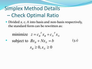
8. Simplex Method Details
– Check Optimal Ratio
 Divided x, c, A into basis and non-basis respectively,
the standard form can be rewritten as:
 (3.1)
minimize
subject to
0, 0
T T
B B N N
B N
B N
z c x c x
Bx Nx b
x x
 
 
 

9. Simplex Method Details
– Check Optimal Ratio
 From the first constraint:
 At optimal point , then .
 Substituting xB into the objective:
 
1
B N
x B b Nx

 
 
 
 
1
1 1
* 1
T T
B N N N
T T T
B N B N
T T T
B B N B N
z c B b Nx c x
c B b c c B N x
c x c c B N x

 

  
  
  
0
N
x  * 1
B
x B b



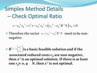
10. Simplex Method Details
– Check Optimal Ratio
 Therefore the vector need to be non-
negative.
 If is a basic feasible solution and if the
associated reduced costs rN are non-negative,
then x* is an optimal solution. If there is at least
one rq < 0, q N, then x* is not optimal.
 
* * 1
0
T T T T T
B B B B N B N
z c x c x c x c c B N x

     
1
T T
N N B
r c c B N

 
*
*
*
B
N
x
x
x
 
  
 
 


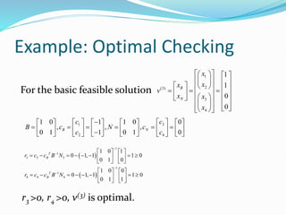
11. Example: Optimal Checking
1 2
1 3
2 4
1 2 3 4
minimize
subject to 1
1
0, 0, 0, 0
x x
x x
x x
x x x x
 
 
 
   
For the basic feasible solution
3
2
(1)
1
4
1
1
0
0
B
N
x
x
x
v
x x
x
 
   
 
   
   
   
  
     
 
     
 
   
 
 
3 1
4
2
1 0 0 1 0 1
, , ,
0 1 1 0 1 0
B N
c c
B c N c
c
c

   
       
     
   
       

       
 
 
 
 
1
1
1 1 1
1
1
4 4 4
1 0 1
1 0, 1 1 0
0 1 0
1 0 0
0 0, 1 1 0
0 1 1
T
B
T
B
r c c B N
r c c B N




   
        
   
   
   
      
   
   
r1 <0, v(1) is not optimal.

12. Example: Optimal Checking
For the basic feasible solution
1
2
(3)
3
4
1
1
0
0
B
N
x
x
x
v
x x
x
 
   
 
   
   
   
  
     
 
     
 
   
 
 
3
1
2 4
1 0 1 1 0 0
, , ,
0 1 1 0 1 0
B N
c
c
B c N c
c c
  
 
       
     
 
 
       

       
   
 
 
1
1
3 3 3
1
1
4 4 4
1 0 1
0 1, 1 1 0
0 1 0
1 0 0
0 1, 1 1 0
0 1 1
T
B
T
B
r c c B N
r c c B N




   
       
   
   
   
       
   
   
r3 >0, r4 >0, v(3) is optimal.

13. Simplex Method Details
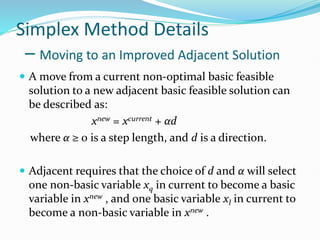
– Moving to an Improved Adjacent Solution
 A move from a current non-optimal basic feasible
solution to a new adjacent basic feasible solution can
be described as:
xnew = xcurrent + αd
where α ≥ 0 is a step length, and d is a direction.
 Adjacent requires that the choice of d and α will select
one non-basic variable xq in current to become a basic
variable in xnew , and one basic variable xl in current to
become a non-basic variable in xnew .

14. Simplex Method Details
– Moving to an Improved Adjacent Solution
 From a start point
to an adjacent point .
 Expanding to the full n dimensions of vectors:
xnew = xcurrent + αd
which suggests direction , where
1 1 1
current
B N B N
Bx Nx b x B b B Nx B b
  
     
1 1 1
new current
B q q B q q
x B b B N x x B N x
  
   
1
0
new current
B B
new current
N N
x x B d
d d
x x
 

     
   
     
     
   
1
q
q
B N
d
e

 

  
 
 
0
0
1
0
q
e n m

 

 

 

 
 

 

 

 

 

 
qth

15. Simplex Method Details
– Moving to an Improved Adjacent Solution
 Theorem 3.1
Suppose x* is basis feasible solution with basic matrix
B and non-basis matrix N. For any non-basic variable
xq with rq < 0, the direction will lead to a
decrease in the objective function.
 Proof: cTxnew = cT(xcurrent + αdq) < cTxcurrent
=> cTdq < 0 (α non-negative)
1
q
q
q
B N
d
e

 

  
 
 
1
1 1
0
T
q
B
T q T T T
B q N q q B q q
N q
B N
c
c d c B N c e c c B N r
c e

 
 

 
       
 
 
   
 

16. Simplex Method Details
– Feasibility of a Descent Direction
 Check xnew = xcurrent + αdq satisfy:
(1) Axnew = b (2) xnew ≥ 0
 To show (1) we consider Axnew = A(xcurrent + αdq) =
Axcurrent + αAdq = b + αAdq = b => Adq = 0.
 To show (2) xnew = xcurrent + αdq ≥ 0
Case 1: if dq ≥ 0, xnew = xcurrent + αdq ≥ 0 for any α ≥ 0.
but cTdq < 0 since rq < 0, cT(xcurrent + αdq) = cTxcurrent +
αcTdq -> -∞ as α -> ∞, therefore the LP is unbounded.
 
1
1
| 0
q
q
q q q q
q
B N
Ad B N BB N Ne N N
e


 

       
 
 
 

17. Simplex Method Details
– Feasibility of a Descent Direction
Case 2: there is at least one component of dq that is
negative. By the requirement xcurrent + αdq ≥ 0 =>
αdq ≥ - xcurrent, thus the largest α is:
where is the index set of basic variables in xcurrent.
The determination of α is called the minimum ratio
test.
min | 0
current
j q
j
q
j B
j
x
d
d


 
 
  
 
 
 
B

18. Simplex Method Details
– Direction and Step Length
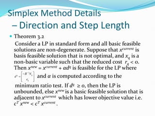
 Theorem 3.2
Consider a LP in standard form and all basic feasible
solutions are non-degenerate. Suppose that xcurrent is
basis feasible solution that is not optimal, and xq is a
non-basic variable such that the reduced cost rq < 0.
Then xnew = xcurrent + αdq is feasible for the LP where
and α is computed according to the
minimum ratio test. If dq ≥ 0, then the LP is
unbounded, else xnew is a basic feasible solution that is
adjacent to xcurrent which has lower objective value i.e.
cT xnew < cT xcurrent .
1
q
q
q
B N
d
e

 

  
 
 

19. Example: Direction and Step Length
1 2
1 3
2 4
1 2 3 4
minimize
subject to 1
1
0, 0, 0, 0
x x
x x
x x
x x x x
 
 
 
   
3
2
(1)
1
4
1
1
0
0
B
current
N
x
x
x
x v
x x
x
 
   
 
   
   
   
   
     
 
     
 
   
 
 
 
1
1
1 1 1
1 0 1
1 0, 1 1 0, is not optimal.
0 1 0
T current
B
r c c B N x

    
        
   
   
1
1
3
1
1
2
1 1
1
1 1
1
4
1
1 0 1
0
0 1 0
1
1
0
0
d
d
B N
d
e d
d


 
  
 
   
 

   
   
 
  
 
     
   
   
   
   
   
 
   
   

20. Example: Direction and Step Length
 Since there is at least one component of d1 is negative,
minimum ratio test for α :
 xnew = xcurrent + αdq =
 cT xnew = -2 < -1 = cT xcurrent
3
1
{3,2}
3
1
min | 0 1
1
current current
j q
j
q
j B
j
x x
d
d d

 
   
   
       
     

 
   
 
3
2
1
4
1 1 0
1 0 1
1
0 1 1
0 0 0
new
new
new
new
x
x
x
x
 

     
 
     
 
     
    
     
 
     
 
       

21. Simplex Method
 Step 0: (Initialization)
Generate an initial basic solution x(0) = [xB | xN]T.
Let B be the basis matrix and N be the non-basis
matrix with corresponding partition c = [cB | cN]T.
Let and be the index sets of xB and xN .
Let k = 0, Go to Step 1.
 Step 1: (Optimality Check)
Compute the reduced cost for all .
If rq ≥ 0 for all , x(k) is optimal, STOP, else select
one xq from non-basis such that rq < 0, Go to Step 2.
B N
1
T
q q B q
r c c B N

  q N

q N


22. Simplex Method
 Step 2: (Descent Direction Generation)
Construct .
If dq ≥ 0, then the LP is unbounded, else Go to Step 3.
 Step 3: (Step Length Generation)
Compute the step length (the mini-
mum ratio test). Let j* be the index of basic variable
then attains the minimum ratio α. Go to Step 4.
 Step 4: (Improved Adjacent Basic Feasible Solution)
Let x(k+1) = x(k) + αdq. Go to Step 5.
1
q
q
q
B N
d
e

 

  
 
 
min | 0
current
j q
j
q
j B
j
x
d
d


 
 
  
 
 
 

23. Simplex Method
 Step 5: (Basis Update)
Let Bj* be the column in B associated with the leaving
basic variable xj*.
Update the basis matrix B by removing Bj* and adding
the column Nq, thus
Update the non-basis matrix N by removing Nq and
adding Bj*, thus
Let k = k+1, Go to Step 1.
   
*
B B j q
 
   
*
N N q j
 

24. Example: Simplex Method
1 2
1 3
2 4
1 2 3 4
minimize
subject to 1
1
0, 0, 0, 0
x x
x x
x x
x x x x
 
 
 
   
Step 0: Initialization
3
4
(0)
1
2
1
1 1 0 1 0
with ,
0 0 1 0 1
0
B
N
x
x
x
x B N
x x
x
 
   
 
   
     
 
   
    
     
   
     
     
 
   
 
 
   
3
4
0 1
, , 3,4 , 1,2
0 1
B N
c
c c B N
c

     
    
     

   
 

25. Example: Iteration 1
 Step 1:
x(0) is not optimal, choose x1 as the non-basis variable
enter the basis. Go to Step 2
 Step 2: Constructed
 Step 3: Compute step length
. Go to Step 4.
 
 
1
1
1 1 1
1
1
2 2 2
1 0 1
1 0,0 1 0
0 1 0
1 0 0
1 0,0 1 0
0 1 1
T
B
T
B
r c c B N
r c c B N




   
       
   
   
   
       
   
   
1
1
1 1
1
1
1 0 1
0
0 1 0
0
1
1
0
0
B N
d
e


  
 
   

   
   
 
  
     
   
     
     
   
 
1 3
1 1
{3,4}
3
1
min | 0 1
1
current current
j
j
j B
j
x x
d
d d

 
   
   
       
     

 
   
 

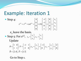
26. Example: Iteration 1
 Step 4:
x3 leave the basis.
 Step 5: For x(1),
Update
Go to Step 1.
3
4
(1) (0) (1)
1
2
1 1 0
1 0 1
(1)
0 1 1
0 0 0
x
x
x x d
x
x

  
     
 
     
 
     
     
 
     
 
     
       
3
1
4 2
,
B N
x
x
x x
x x
 
 
   
 
   
   
3
1
4 2
1 0 1 0 1 0
, , ,
0 1 0 1 0 1
1,4 , 3,2
B N
c
c
B N c c
c c
B N
  
 
       
     
 
 
       

       
   
 

27. Example: Iteration 2
 Step 1:
x(1) is not optimal, choose x2 as the non-basis variable
enter the basis. Go to Step 2
 Step 2: Constructed
 Step 3: Compute step length
. Go to Step 4.
 
 
1
1
3 3 3
1
1
2 2 2
1 0 1
0 1,0 1 0
0 1 0
1 0 0
1 1,0 1 0
0 1 1
T
B
T
B
r c c B N
r c c B N




   
      
   
   
   
        
   
   
1
1
2 2
2
0
1 0 0
1
0 1 1
0
0
0
1
1
B N
d
e


   
   

   
   
  
  
     
   
     
     
   
 
2 4
2 1
{1,4}
4
1
min | 0 1
1
current current
j
j
j B
j
x x
d
d d

 
   
   
       
     

 
   
 

28. Example: Iteration 2
 Step 4:
x4 leave the basis.
 Step 5: For x(2),
Update
Go to Step 1.
1
4
(2) (1) (2)
3
2
1 0 1
1 1 0
(1)
0 0 0
0 1 1
x
x
x x d
x
x

 
     
 
     
  
     
     
 
     
 
     
       
3
1
2 4
,
B N
x
x
x x
x x
 
 
   
 
   
   
3
1
2 4
1 0 1 0 1 0
, , ,,
0 1 0 1 1 0
1,2 , 3,4
B N
c
c
B N c c
c c
B N
  
 
       
     
 
 
       

       
   
 

29. Example: Iteration 3
 Step 1:
rN ≥ 0, STOP. x(2) is optimal.
 The path of the iterations is
v(0) -> v(2) -> v(3)
 If we chose x2 as enter vari-
able in iteration 1, the path
will be v(0) -> v(1) -> v(3)
 
 
1
1
3 3 3
1
1
4 4 4
1 0 1
0 1, 1 1 0
0 1 0
1 0 0
0 1, 1 1 0
0 1 1
T
B
T
B
r c c B N
r c c B N




   
       
   
   
   
       
   
   

30. Initial Basis Generation
– Two Phase Method
 Artificial variables
In the case where it is difficult to identify identity sub-
matrix, in the constraint set Ax = b, one can add
artificial variables to create an identity sub-matrix.
 E.g. x1 + 2x2 + x3 + x4 = 4
-x1 - x3 - x5 = 3
The basis is hard to find, we add x6 and x7 to the
constraints,
x1 + 2x2 + x3 + x4 + x6 = 4
-x1 - x3 - x5 + x7 = 3
1 2 1 1 0 1 0 4
,
1 0 1 0 1 0 1 3
A b
   
 
   
  
   

31. Initial Basis Generation
– Two Phase Method
 Consider a standard form of a Linear Programming (SFLP)
And consider the addition of artificial variables (ALP)
 The relationship between SFLP and ALP as follows:
(1) If SFLP has a feasible solution, then ALP has a feasible
solution with xa = 0.
(2) If ALP has a feasible solution with xa = 0, then SFLP has
a feasible solution.
minimize
subject to
0
T
c x
Ax b
x


minimize
subject to
0
T
a
c x
Ax x b
x
 


32. Initial Basis Generation
– Two Phase Method
 Phase I:
The Phase I problem can be initialized with the basic
solution x = 0, xa = b.
Let be the optimal solution to Phase I.
 Case 1: If xa
* ≠ 0, then the original LP is infeasible.
 Case 2: otherwise xa
* = 0 with 2 sub-cases:
minimize 1
subject to
0, 0
T
a
a
a
x
Ax x b
x x
 
 
*
*
a
x
x
x
 
  
 
 

33. Initial Basis Generation
– Two Phase Method
 Subcase 1: All xa
* in the non-basis, then discard the
artificial variables in ALP and use the x* as a starting
solution for Phase II problem:
 Subcase 2: Some of the artificial variables are basic
variables. Then exchange such an artificial basic
variable with a current non-basis and non-artificial
variables xq. Let xa
*i be such artificial variable in the jth
position among xB. There are 2 sub-subcases:
minimize
subject to
0, 0
T T
B B N N
B N
B N
c x c x
Bx Nx b
x x

 
 

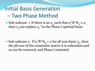
34. Initial Basis Generation
– Two Phase Method
 Sub-subcase 1: If there is an xq such that ej
TB-1Nq ≠ 0,
then xq can replace xa
*i in the Phase I optimal basis.
 Sub-subcase 2: If ej
TB-1Nq = 0 for all non-basic xq, then
the jth row of the constraint matrix A is redundant and
so can be removed, and Phase I restarted.

35. Example: Two Phase Method
 Phase I:
1 2
1 2
1 2
1 2
1 2
minimize 2
subject to 2
2 3
2 4
0, 0
x x
x x
x x
x x
x x

 
  
 
 
6 7 8
1 2 3 6
1 2 4 7
1 2 5 8
1 2 3 4 5 6 7 8
minimize
subject to + 2
2 + 3
2 + 4
, , , , , , , 0
x x x
x x x x
x x x x
x x x x
x x x x x x x x
 
  
   
  


36. Example: Two Phase Method
 Solving Phase I by simplex method gives optimal
solution
1 1
6 6 2 2
7 7 3 3
8 8 4 4
5 5
0 0
2 1 0 0
3 , 1 , 0 , 0
4 1 0 0
0 0
1 0 0 1 1
0 1 0 ,
0 0 1
B B N N
x c
x c x c
x x b c c x x c c
x c x c
x c
B N
   
   
   
   
   
       
   
   
       
   
        
   
       
   
   
   
   
       
   
   
   
   
   

 
 
 
 
 
 
   
1 0 0
1 2 0 1 0
2 1 0 0 5
6,7,8 , 1,2,3,4,5 ,
B N
 
 
 
 
 
 
 
   
1
* *
2 4 5 6 7 8
3
1
2 , 0 0 0 0 0
1
T T
B N
x
x x x x x x x x
x
   
   
   
   
   
 
 

37. Example: Two Phase Method
 xa
* = [x6, x7, x8]T = [0 0 0]T, and are all in non-basis,
then reformulate Phase II problem:
 And use the initial basic feasible solution x* from
Phase I, we finally get the optimal solution:
x1 = 1/3, x2 = 5/3, x3 = 1, x4 = 0, x5 = 5/3,
1 2
1 2 3
1 2 4
1 2 5
1 2 3 4 5
minimize 2
subject to 2
2 3
2 4
, , , , 0
x x
x x x
x x x
x x x
x x x x x

  
   
  


38. Initial Basis Generation
– Big M Method
 The Big M problem is
where M > 0 is a large parameter.
 The Big M problem can be solved by the Simplex
Method with the initial basic feasible solution xa = b as
basic variables and x = 0 as the non-basic variables.
 One of two cases will be resulted in by Big M method:
minimize 1
subject to
0, 0
T T
a
a
a
c x M x
Ax x b
x x

 
 

39. Initial Basis Generation
– Big M Method
 Case 1: Solving the Big M model results in a finite
optimal solution
Subcase 1: If xa
* = 0, then x* is the optimal for the
original LP.
Subcase 2: If xa
* ≠ 0, then the original LP is infeasible.
 Case 2: The Big M problem is unbounded below.
Subcase 1: If xa
* = 0, then the original LP is also
unbounded below.
Subcase 2: If at least one artificial variable is non-
zero, then the original LP is infeasible.
*
*
a
x
x
x
 
  
 
 

40. Example: Big M Method
 Solving by Simplex method, the optimal solution is:
x1 = 1/3, x2 = 5/3, x3 = 0, x4 = 0, x5 = 5/3,
x6 = 0, x7 = 0, x7 = 0.
 Since xa
* = [x6, x7, x8]T = [0 0 0]T, the solution is
optimal to original LP.
1 2 6 7 8
1 2 3 6
1 2 4 7
1 2 5 8
1 2 3 4
minimize 2
subject to + 2
2 + 3
2 + 4
, , , ,
x x Mx Mx Mx
x x x x
x x x x
x x x x
x x x x x
   
  
   
  
5 6 7 8
, , , 0
x x x 

41. Degeneracy
 It is possible for basic feasible solutions has some basic
variables with zeros values i.e. these basic feasible
solution are degenerate.
 Suppose xd be a degenerate basic feasible solution, and
xnew = xd + αdq is feasible, i.e.
Axnew = b xnew = xd + αdq ≥ 0
since some of the basic variables in xd are zero, then
the minimum ratio test may set α to 0. In such case,
the value of xnew and xd are same, and there is no
improvement in objective value. However, xnew is
distinct from and adjacent to xd.

42. Example: Degeneracy
 Consider the constraints
x1 + x2 ≤ 40
2x1 + x2 ≤ 40
x2 ≤ 40
x1 ≥ 0 x2 ≥ 0

43. Cycling
 It is possible that the Simplex Method return a basic
feasible solution that was visited in the previous
iterations, i.e. cycling occurs.
 Beale’s (1955) example
4 5 6 7
1 4 5 6 7
2 4 5 6 7
3 6
1 1
minimize 20 6
4 2
1
subject to 8 9 0
4
1 1
12 3 0
2 2
1
x x x x
x x x x x
x x x x x
x x
   
    
    
 
1 2 3 4 5 6 7
, , , , , , 0
x x x x x x x 

44. Cycling
 Using initial B associated with x1, x2 and x3, the
following iterations are obtained:
iteration Enter
variable
Leaving
variable
Basic variables Obj val
0 x1=0, x2=0, x3=1, 0
1 x4 x1 x4=0, x2=0, x3=1, 0
2 x5 x2 x4=0, x5=0, x3=1, 0
3 x6 x4 x6=0, x5=0, x3=1, 0
4 x7 x5 x6=0, x7=0, x3=1, 0
5 x1 x6 x1=0, x7=0, x3=1, 0
6 x2 x7 x1=0, x2=0, x3=1, 0

45. Anti-Cycling Rules
– Bland’s Rule
 Bland’s Rule:
(1)For non-basic variables with negative reduced costs,
select the variables with smallest index to enter the
basis.
(2)If there is a tie in the minimum ratio test select the
variables with smallest index to leave the basis.
 Bland (1977) proof that if the Simplex Method uses
Bland’s Rule, then the Simplex Method will not cycle.

46. Anti-Cycling Rules
– Bland’s Rule
 Starting from iteration 4, the iterations are different
when using Bland’s rule.
iteration Enter
variable
Leaving
variable
Basic variables Obj val
0 x1=0, x2=0, x3=1, 0
1 x4 x1 x4=0, x2=0, x3=1, 0
2 x5 x2 x4=0, x5=0, x3=1, 0
3 x6 x4 x6=0, x5=0, x3=1, 0
4 x1 x5 x6=0, x1=0, x3=1, 0
5 x2 x3 x6=1, x1=1, x2=1/2, -1/2
6 x4 x2 x6=1, x1=3/4, x4=1, -5/4

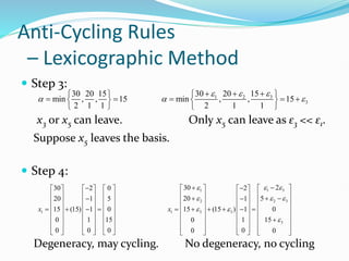
47. Anti-Cycling Rules
– Lexicographic Method
 Dantzig et al. (1955) present Lexicographic Method
which is to eliminate degeneracy, and finally prevent
the cycling.
 Consider LP:
 Assign a small positive constant εi to the RHS of ith
constraint with the order 0 << εm << … << ε2 << ε1.
1 1
2 2
minimize
subject to
0
T
T
T
T
m m
c x
a x b
a x b
a x b
x





48. Anti-Cycling Rules
– Lexicographic Method
 Adding such constants to the right hand side will
ensure that there is a unique variable to leave the basis
during an iteration
 The enter variable can be selected any non-basic
variables with negative reduced cost.
1 1 1
2 2 2
minimize
subject to
0
T
T
T
T
m m m
c x
a x b
a x b
a x b
x



 
 
 


49. Anti-Cycling Rules
– Lexicographic Method
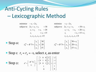
 Step 0:
 Step 1: r1 = r2 = -1, select x1 as enter
 Step 2:
1 2 1 2
1 2 3 1 2 3 1
1 2 4
minimize 2 minimize 2
subject to 2 30 subject to 2 30
20
x x x x
x x x x x x
x x x

   
      
   1 2 4 2
1 5 1 5 3
1 2 3 4 5
20
15 15
, , , , 0
x x x
x x x x
x x x x x


   
    
 1 2 3 4 5
, , , , 0
x x x x x 
3 3 1
(0) 1 (0) 1
4 4 2
5 5 3
30
30
20 20
15 15
B B
x x
x B b x x B b x
x x



 

     
 
     
 
      
     
 
     
  
   
   
1
1 1
1
1 0 0 2 2
0 1 0 1 1
0 0 1 1 1
1
1
0
0
B N
d
e

  
     
 
     
 
 
     
 

 
     
   
     
   
 
   
   
 
 

50. Anti-Cycling Rules
– Lexicographic Method
 Step 3:
x3 or x5 can leave. Only x5 can leave as ε3 << ε1.
Suppose x5 leaves the basis.
 Step 4:
Degeneracy, may cycling. No degeneracy, no cycling
3
1 2
3
15
30 20
30 20 15
min , , 15 min , , 15
2 1 1 2 1 1

 
  

 
 
 
    
   
   
1 3
1
2 3
2
1 1 3 3
3
2
30
30 2 0 2
5
20
20 1 5 1
15 (15) 1 0 15 (15 ) 1 0
0 1 15 1 15
0
0 0 0 0
0 0
x x
 

 

 



  
 
       

 
         

 
 
       
 
       
         
 
       

 
       
 
       
       
  


 
 
 
 
 


51. Anti-Cycling Rules
– Lexicographic Method
 Theorem 3.3
Assume that the constraint matrix of a linear program
has full row rank m. If the leaving variable is
determined by Lexicographic Method, then the
Simplex Method will always terminate.

52. Revised Simplex Method
 Simplex Method require the basis B is invertible
during iteration, this is computational expensive in
practice.
 A better idea is to generate an inverse B-1 by solving an
equivalent linear system of equations.
 For example, to compute the reduced costs the linear
system BTπ = cB is solved first for and then the vector
rN = cN – πTN can be easily computed.
 In practice, triangular factorization such as LU decom-
position to solve the square system can enhance both
the numerical stability and reduce space requirement

53. Revised Simplex Method
 Step 0: (Initialization)
Generate an initial basic solution x(0) = [xB | xN]T.
Let B be the basis matrix and N be the non-basis
matrix with corresponding partition c = [cB | cN]T.
Let and be the index sets of xB and xN .
Let k = 0, Go to Step 1.
 Step 1: (Optimality Check)
Solve for π in the linear system BTπ = cB.
Compute the reduced cost rq = cq - π TNq for all .
If rq ≥ 0 for all , x(k) is optimal, STOP, else select
one xq from non-basis such that rq < 0, Go to Step 2.
B N
q N

q N


54. Revised Simplex Method
 Step 2: (Descent Direction Generation)
Solve for d in the linear system Bd = -Nq.
Construct .
If dq ≥ 0, then the LP is unbounded, else Go to Step 3.
 Step 3: (Step Length Generation)
Compute the step length (the minimum
ratio test). Let j* be the index of basic variable
then attains the minimum ratio α. Go to Step 4.
 Step 4: (Improved Adjacent Basic Feasible Solution)
Let x(k+1) = x(k) + αdq. Go to Step 5.
1
q
q
q
B N
d
e

 

  
 
 
min | 0
current
j q
j
q
j B
j
x
d
d


 
 
  
 
 
 

55. Revised Simplex Method
 Step 5: (Basis Update)
Let Bj* be the column in B associated with the leaving
basic variable xj*.
Update the basis matrix B by removing Bj* and adding
the column Nq, thus
Update the non-basis matrix N by removing Nq and
adding Bj*, thus
Let k = k+1, Go to Step 1.
   
*
B B j q
 
   
*
N N q j
 

56. Example: Revised Simplex Method
1 2
1 2 3
1 2 4
1 2 3 4
minimize 2
subject to 4
2 6
0, 0, 0, 0
x x
x x x
x x x
x x x x

   
  
   
Step 0: Initialization
3
4
(0)
1
2
4
6 1 0 1 1
with ,
0 0 1 2 1
0
B
N
x
x
x
x B N
x x
x
 
   
 
    
     
 
   
    
     
   
     
     
 
   
 
 
   
3
4
0 2
, , 3,4 , 1,2
0 1
B N
c
c c B N
c
     
    
     

   
 

57. Example: Iteration 1
 Step 1: Solve BTπ = cB i.e.
x(0) is not optimal, choose x2 as enter. Go to Step 2
 Step 2: Solve Bd = -Nq i.e.
 Step 3: Compute step length
. Go to Step 4.
   
1 1 1 2 2 2
1 1
2 0,0 2 0; 1 0,0 1 0
2 1
T T
r c N r c N
 

   
             
   
   
2
2
1
1
0
0
1
d
d
e

 
 

   
  
   
 
 
 
2 3 3
2 2 2
{3,4}
3 4
4 6
min | 0 , , 4
1 1
current current current
j
j
j B
j
x x x
d
d d d

 
   
   
         
     
 
 
   
 
1 1
2 2
1 0 0 0
0 1 0 0
T
 

 
   
     
   
   
     
     
   
1 1
2 2
1 0 1 1
0 1 1 1
d d
d
d d

   
     
    
   
     

     
   

58. Example: Iteration 1
 Step 4:
x3 leave the basis.
 Step 5: For x(1),
Update
Go to Step 1.
3
4
(1) (0) (1)
1
2
4 1 0
6 1 2
(4)
0 0 0
0 1 4
x
x
x x d
x
x

  
     
 
     
  
     
     
 
     
 
     
       
1
2
3
4
,
B N
x
x
x x
x
x
 
 
   
 
   
   
1
2
3
4
1 0 1 1 1 2
, , ,
1 1 2 0 0 0
2,4 , 1,3
B N
c
c
B N c c
c
c
B N
   
 
       
     
 
 
       
       
   
 

59. Example: Iteration 2
 Step 1: Solve BTπ = cB i.e.
rN ≥ 0, STOP. x(1) is optimal.
   
1 1 1 3 3 3
1 1
2 1,0 1 0; 0 1,0 1 0
2 0
T T
r c N r c N
 

   
             
   
   
1 1
2 2
1 1 1 1
0 1 0 0
T
 

 
 
   
     
   
   
     
     
   

60. Complexity of the Simplex Method
 Definition:
A function g(n) = O(f(n)) (or Big-O of f(n) if there is
constant C > 0 such that for sufficiently large n)
g(n) ≤ Cf(n)
 E.g. the polynomial g(n) = 2n2 +3n +4 = O(n2)
since g(n) ≤ 4f(n) = 4n2 for n ≥ 3 where f(n) = n2.
 For LP (or any problem), an algorithm is said to have
polynomial time worst case complexity if the number of
the operations required in the worst case is a polynomial
function of the size of the problem.
 An algorithm is said to be exponential if the worst case
complexity grows exponentially in the size of the problem.

61. Klee-Minty Problems
 Klee and Minty (1972) shows following LP with 2m
variables and m constraints in standard form
 The simplex method has to enumerate all possible
selection of m variables out of the 2m variables i.e. .
 If m = 50, then that will take 3 trillion years to
finished by a computer with capacity of 1 billion iterations
per second.
1
1
1
1
minimize 10
subject to 2 10 100 , 1,...,
0, , 0
m m j
j
j
i i j i j
j i
j
m
x
x x i m
x x


  

   
 


2m
m
 
 
 
29
100
10
50
 

 
 

62. Simplex Method MATLAB Code
 The standard LP can be solved by
function [xsol objval iter exitflag]=SimplexMethod(c, Aeq, beq, B_set)
 Inputs:
c = n×1 vector, objective coefficient
Aeq = m×n matrix with m < n
beq = m×1 vector, RHS
B_set = m×1 vector, subscript set of basis
 Outputs:
xsol = n*1 vector, final solution
objval is a scalar, final objective value
iter including all iteration details
exitflag describes the exit condition of the problem as follows:
0 - optimal solution
1 - unbounded problem

63. Example 1: Bounded
 minimize –x1 – x2 minimize –x1 – x2
subject to x1 ≤ 1 subject to x1 + x3 = 1
x2 ≤ 1 => x2 + x4 = 1
x1 ≥ 0, x2 ≥ 0 x1 ≥ 0, x2 ≥ 0, x3 ≥ 0, x4 ≥ 0
 Solve by following MATLAB code:
>> c = [-1; -1; 0; 0;];
>> Aeq = [1 0 1 0; 0 1 0 1]; Beq = [1; 1];
>> B_set = [3; 4]; % the subscript of basic variables
>> [xsol fval iter_detail exitflag]=SimplexMethod(c, Aeq, beq, B_set)
probelm solved
xsol = [1 1 0 0]T
fval = -2
iter_detail = [1x1 struct] [1x1 struct] [1x1 struct]
exitflag = 0

64. Example 2: Unboundedness
 minimize –x1 – x2
subject to –2x1 + x2 + x3 = 1
x1 – x2 + x4 = 1
x1 ≥ 0, x2 ≥ 0, x3 ≥ 0, x4 ≥ 0
 Solve by following MATLAB code:
>> c=[-1; -1; 0; 0;];
>> Aeq=[-2 1 1 0; 1 -1 0 1]; beq=[1;1];
>> B_set=[3; 4]; % the subscript of basic variables
>> [xsol fval iter_detail exitflag]=SimplexMethod(c, Aeq, beq, B_set)
unbounded problem
xsol = []
fval = []
iter_detail = []
exitflag = 1