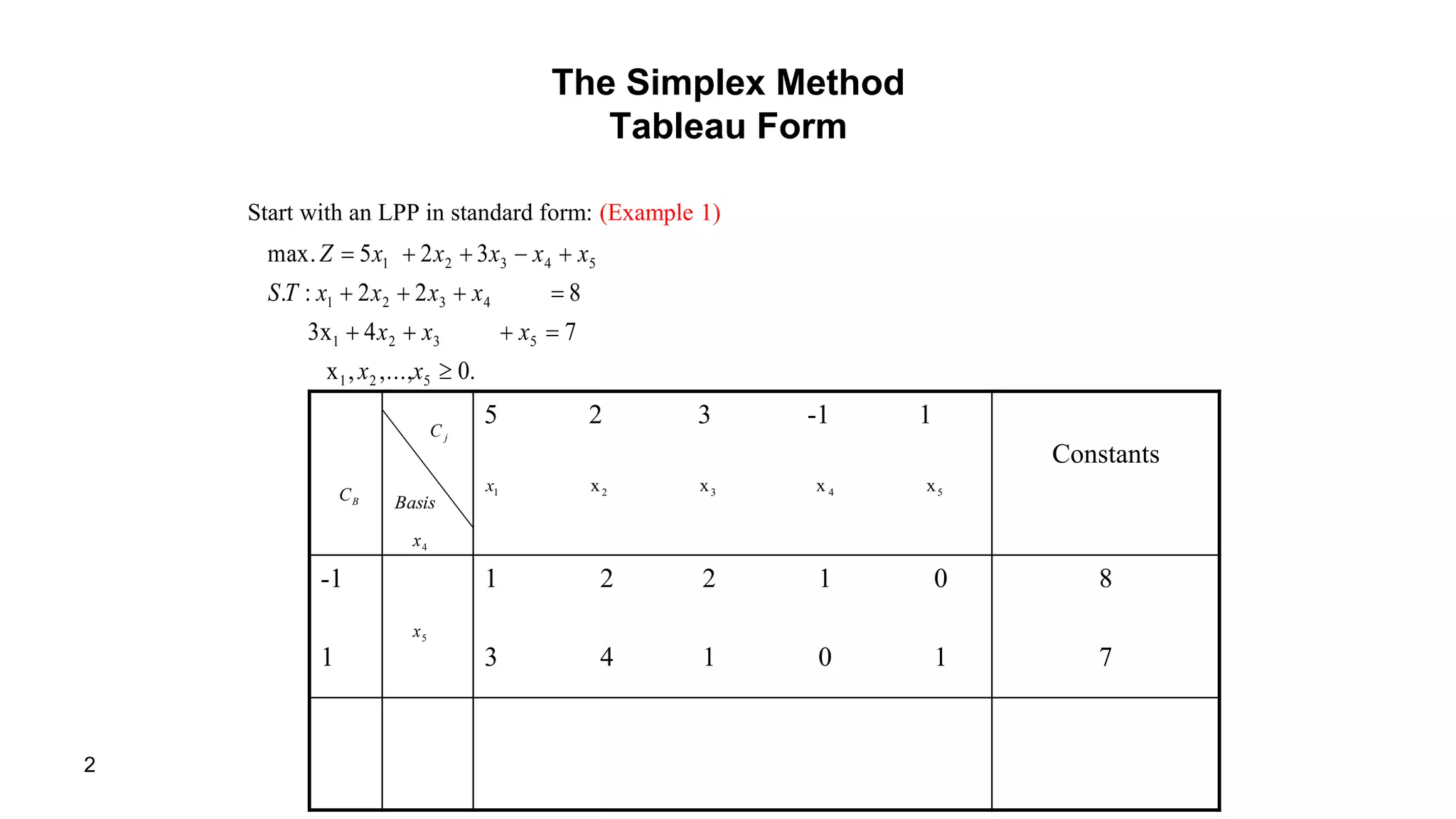
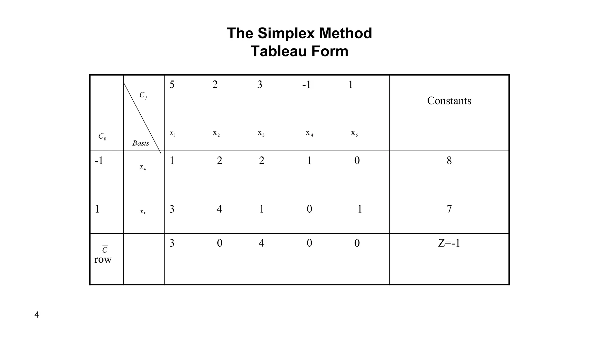
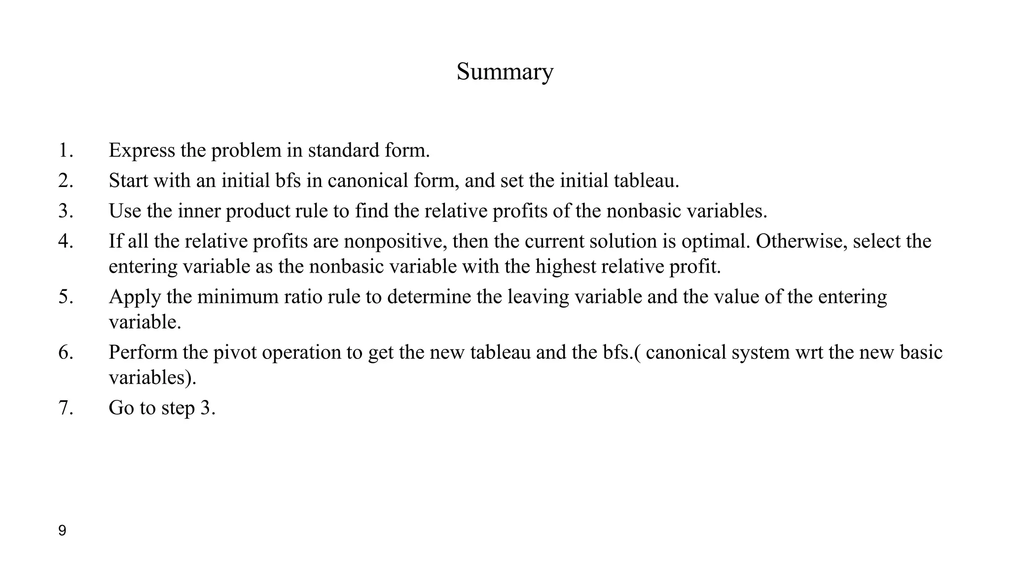
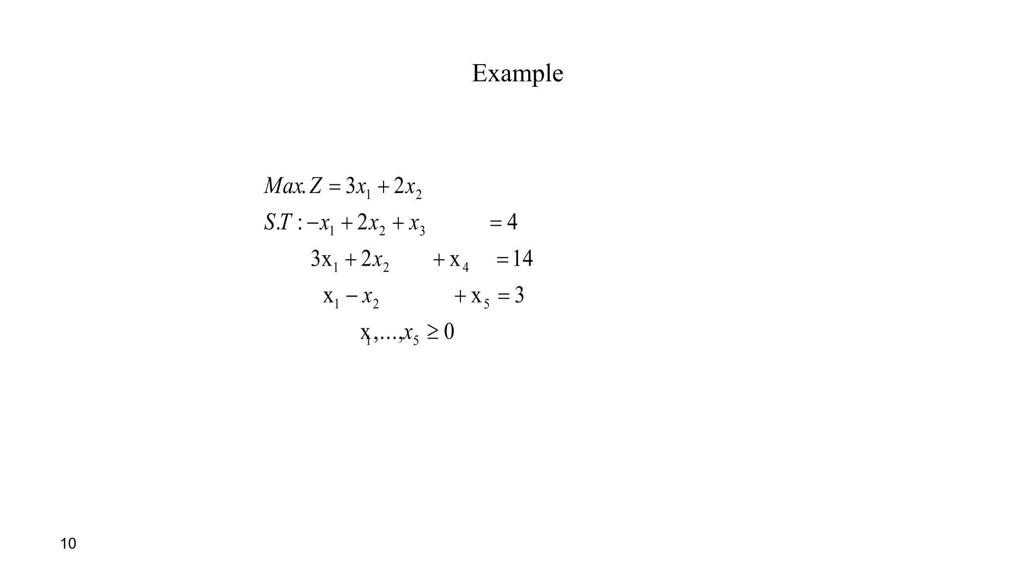
1. The document describes using a tableau form to solve linear programs with the simplex method. It shows how to set up the initial tableau and transform it through iterations.
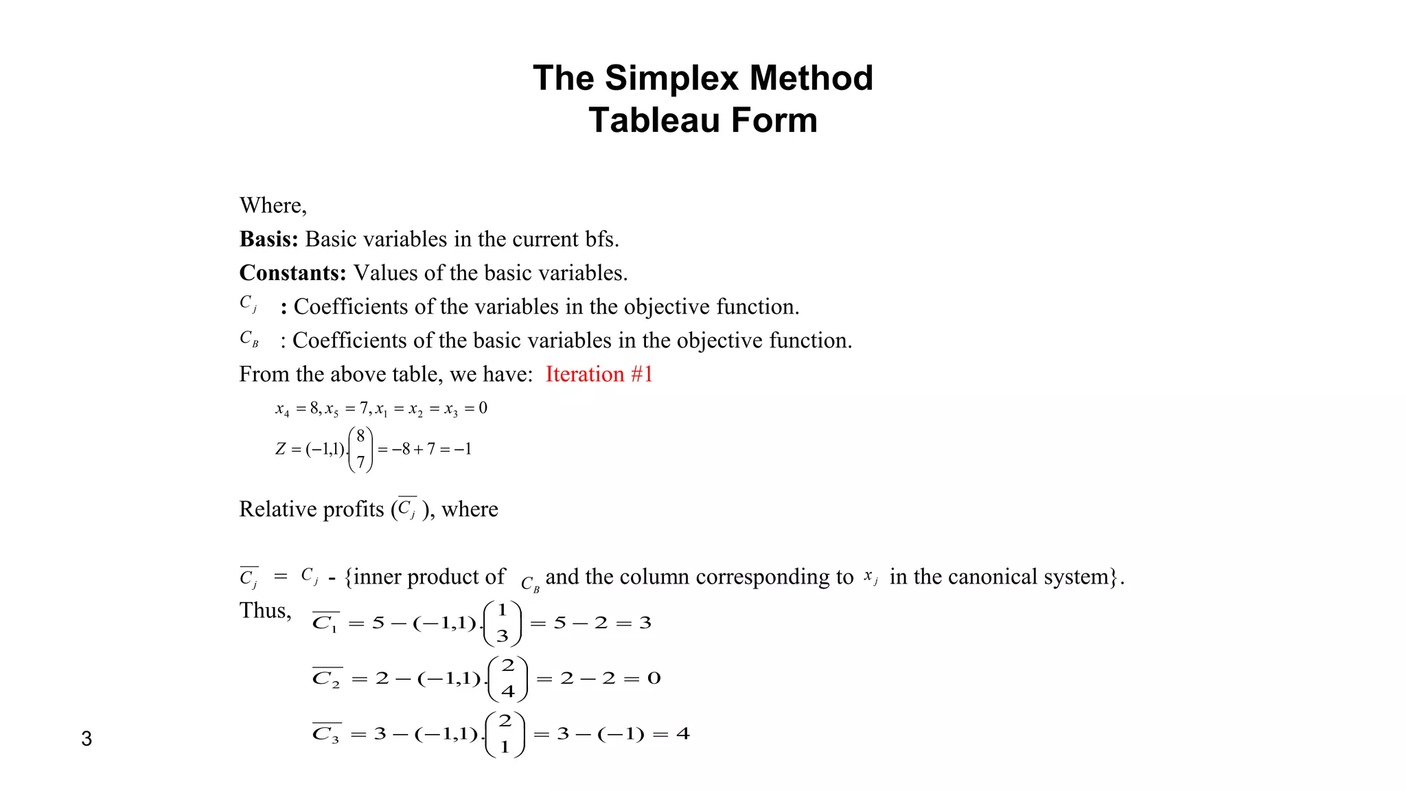
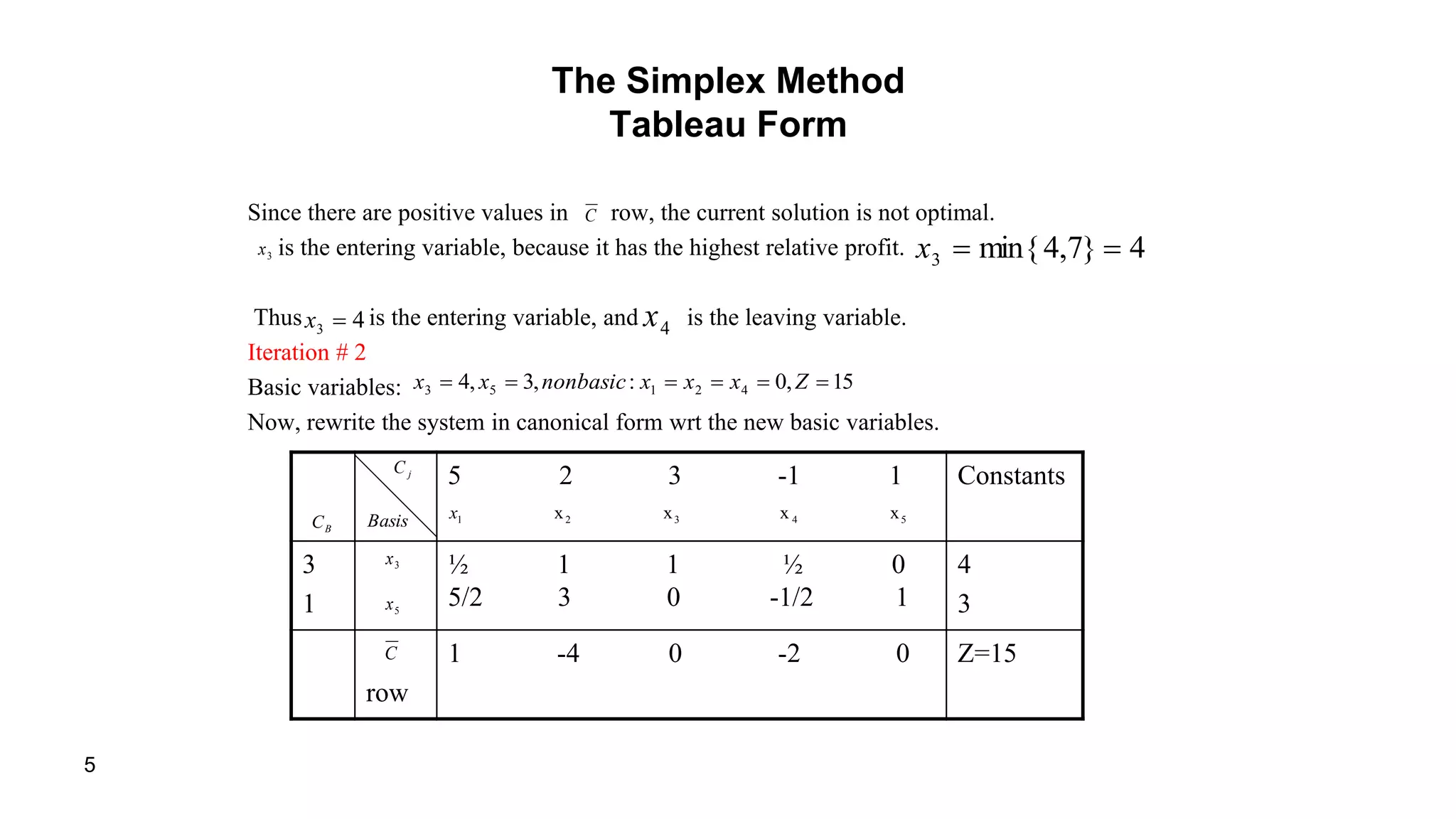
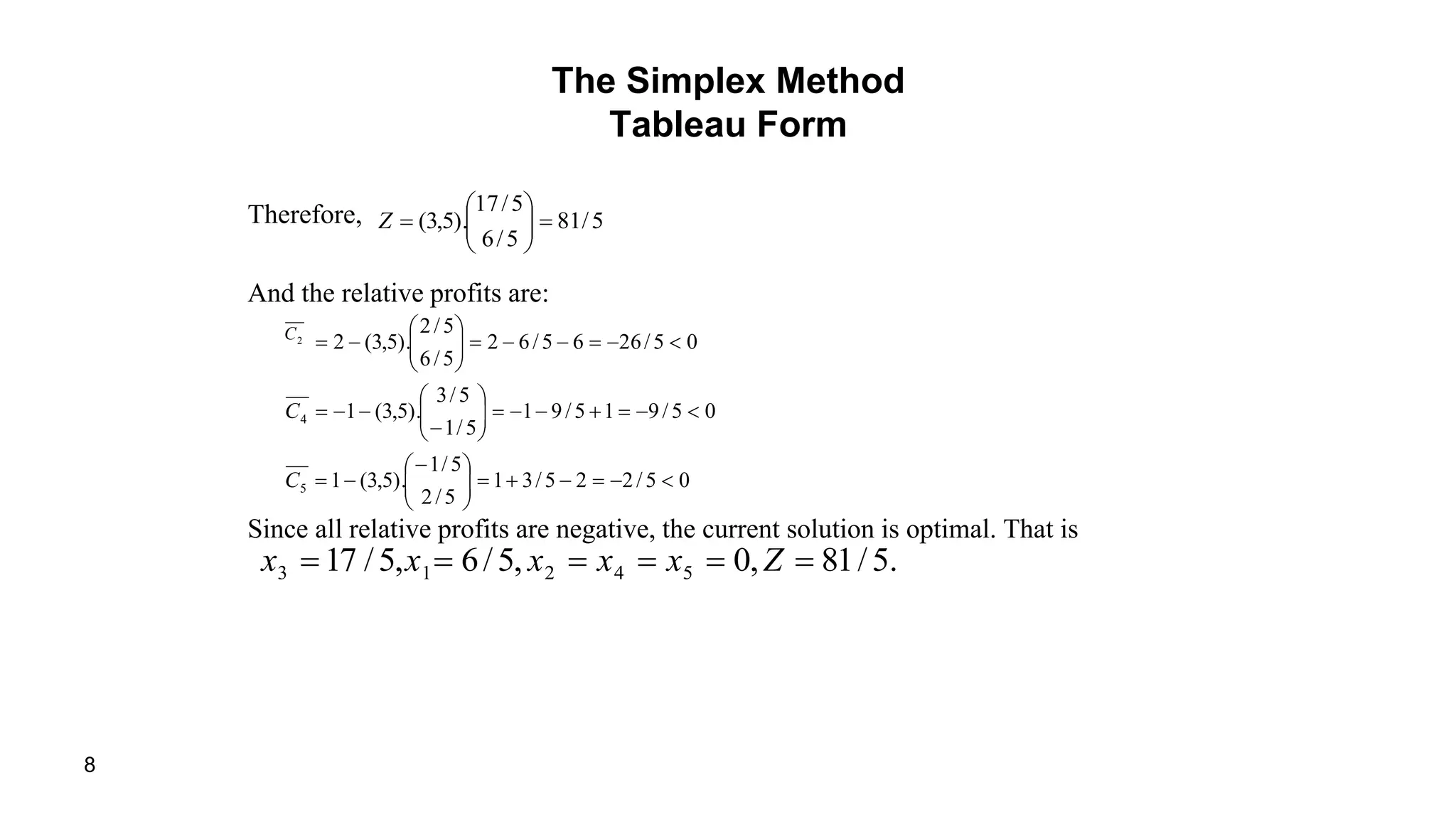
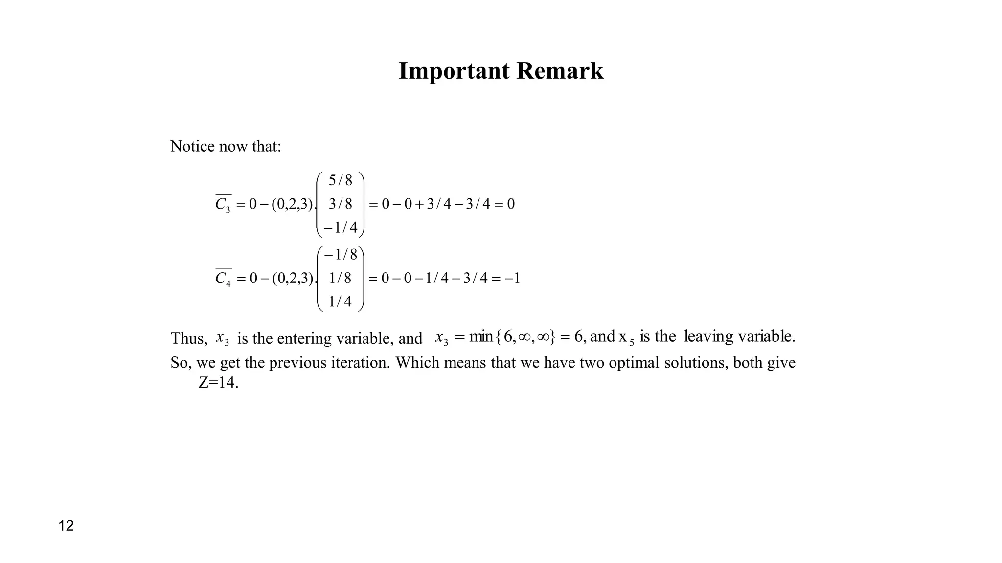
2. Each iteration involves finding the relative profits to determine the entering variable, using the minimum ratio test to find the leaving variable, and updating the tableau to reflect the pivot.
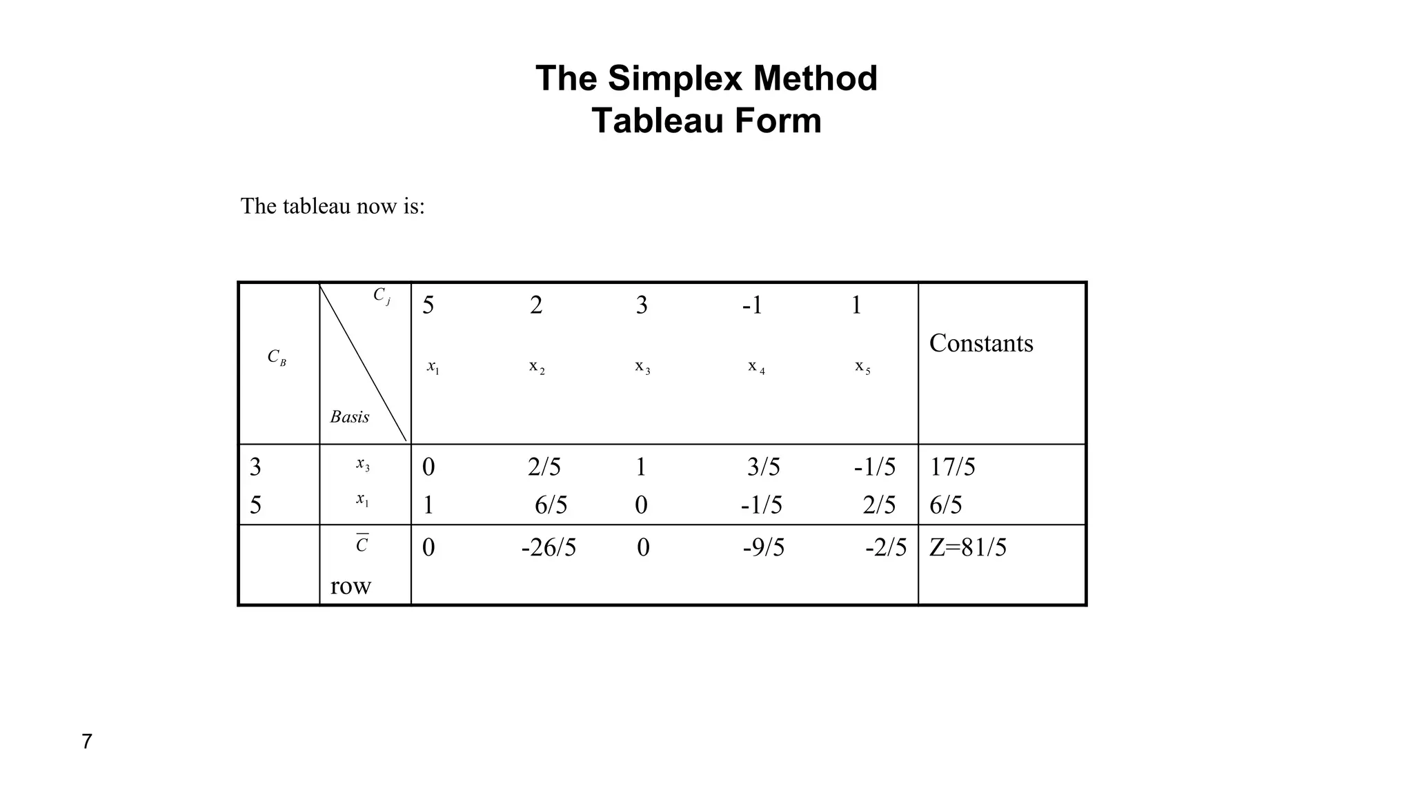
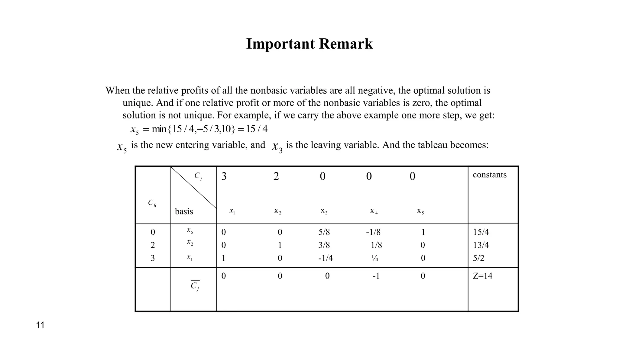
3. The process repeats until an optimal solution is found when all relative profits are nonpositive for maximization or nonnegative for minimization.

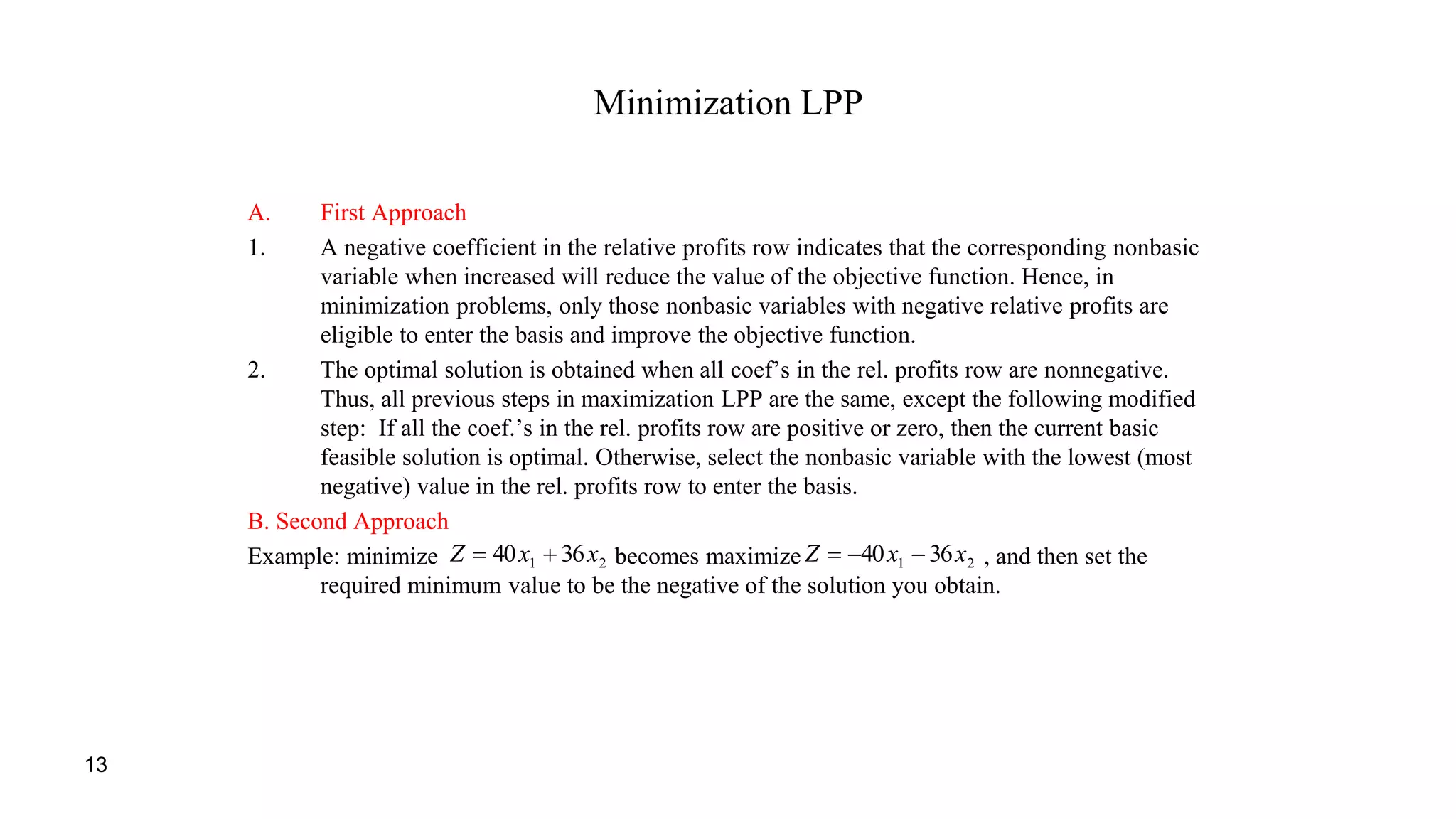


![Mech vii-operation research [06 me74]-notes](https://cdn.slidesharecdn.com/ss_thumbnails/mech-vii-operationresearch06me74-notes-130308221101-phpapp02-thumbnail.jpg?width=640&height=640&fit=bounds)