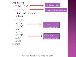
The document outlines the bisection method, a derivative-based optimization technique requiring continuity of the first derivative and unimodal functions. It describes the steps to implement the method, including initializing the level of uncertainty, finding the midpoint, and iterating until a solution is found. An example is provided to illustrate the procedure for determining the minima of a function.

1. NUMERICAL ON
BISECTION METHOD
BY Sumita Das

2. Bisection Method
 It is a Derivative Based Method for Optimization
 Requirements for Bisection Method
 f -> c’ i.e. f is continuous for the first derivative.
 There exists a minima in the level of uncertainty [a
b]
 Function must be unimodal.
PowerPoint Presentation by Sumita Das, GHRCE

3. Algorithm
 Initialize Level of uncertainty [a b]
k=1
ak =a
bk =b
ϵ > 0
l : Allowable level of uncertainty such that
(1/2) n <= (1/(b`-a`))
PowerPoint Presentation by Sumita Das, GHRCE

4. While k<= n
ck= (ak +bk )/2
if f(ck)=0
Stop with ck as the
solution
if f(ck)>0
ak+1 = ak
bk+1 = ck
else
ak+1 = ck
bk+1 = bk
end if
k=k+1
end while
Find midpoint
c is now b.
a remains same
c is now a.
b remains same
Midpoint is the minima
PowerPoint Presentation by Sumita Das, GHRCE

5. In Simple words
Midpoint
m
a b
Example: f(x)=3x2 – 2x
f’(x)=6x-2
Put midpoint value in
derivative.
f’(x)=6*50-2=298
1. if f(m)=0, Midpoint is
minima
2. if f(m)>0, Level of
uncertainty will be [a, m]
3. if f(m)<0, Level of
uncertainty will be [m, b]
50 9010
So, 298>0, level of uncertainty will be
[10, 50] ,Follow the procedure.
PowerPoint Presentation by Sumita Das, GHRCE

6. Example
Que: Find Minima f(x)=(x-2)2
[0 6]
Solution: f ‘(x)=2x-4
k ak bk ck f’(ck )
1 0 6 3 2
2 0 3 1.5 -1
3 1.5 3 2.25 0.5
4 1.5 2.25 1.875 -0.25
5 1.875 2.25 2.062 0.123
6 1.875 2.062 1.9685 -0.063
7 1.9685 2.062 2.015 0.0305
8 1.9685 2.015 1.99175 -0.016
9 1.99175 2.015 2.003 0.006
PowerPoint Presentation by Sumita Das, GHRCE

7. References
[1] Singiresu S. Rao, “Engineering Optimization, Chapter 5:
Nonlinear Programming I: One-Dimensional Minimization
Methods”, 4th Edition
PowerPoint Presentation by Sumita Das, GHRCE