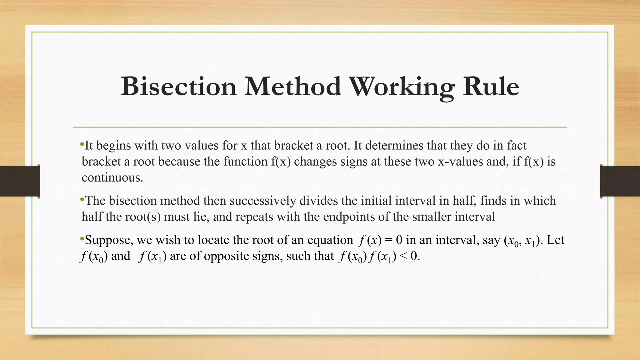
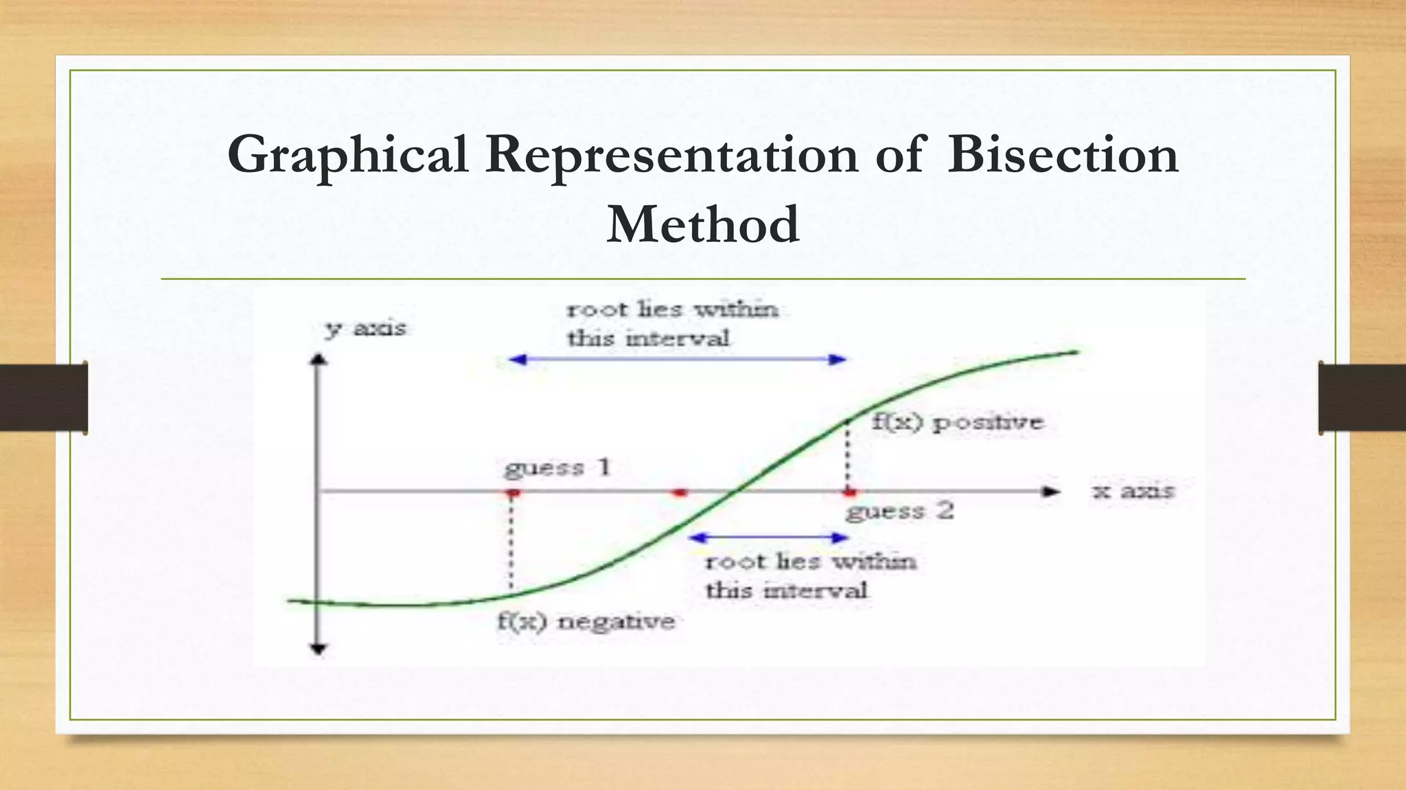
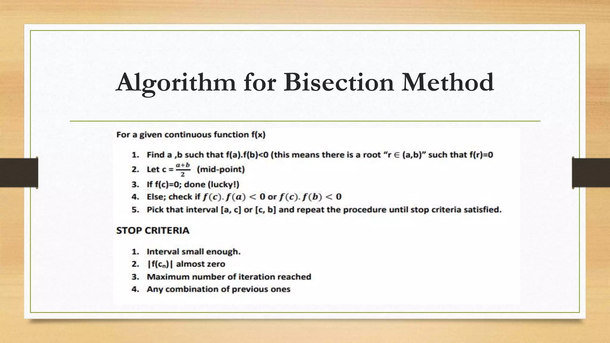
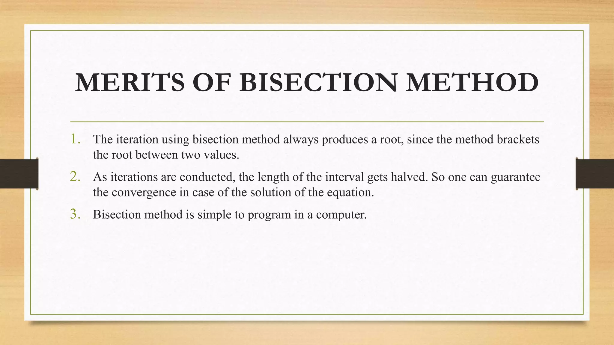
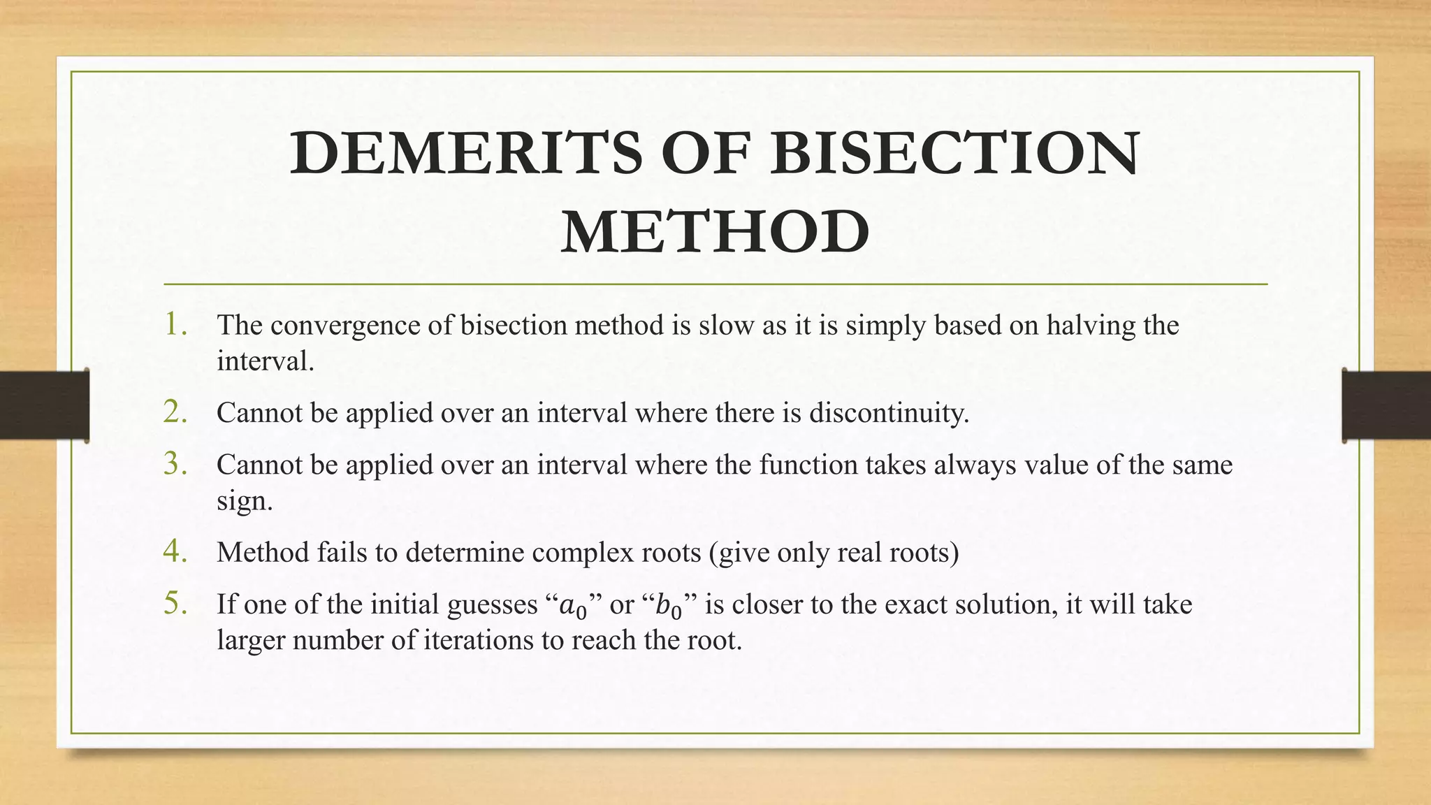
Numerical Computing
Bisection Method
Lecture # 9
By Nasima Akhtar
Bisection Method Working Rule
•It begins with two values for x that bracket a root. It determines that they do in fact
bracket a root because the function f(x) changes signs at these two x-values and, if f(x) is
continuous.
•The bisection method then successively divides the initial interval in half, finds in which
half the root(s) must lie, and repeats with the endpoints of the smaller interval
•Suppose, we wish to locate the root of an equation f (x) = 0 in an interval, say (x0, x1). Let
f (x0) and f (x1) are of opposite signs, such that f (x0) f (x1) < 0.
Graphical Representation of Bisection
Method
Formula Derivation
𝑥2=
𝑥0 + 𝑥1
2
If f (x2) = 0, then x2 is the desired root of f (x) = 0.
However, if f (x2) ≠ 0 then the root may be between x0 and x2 or x2 and x1.
• As we know f(𝑥0)> 0 then, we can find which value to replace for next iteration by the
following condition such as
• If f(𝑥0)*f(𝑥2) < 0 then, 𝑥1= 𝑥2 else 𝑥0= 𝑥2
General form of this method is given by:
𝑥𝑛 =
𝑥𝑛−2 + 𝑥𝑛−1
2
Algorithm for Bisection Method
MERITS OF BISECTION METHOD
1. The iteration using bisection method always produces a root, since the method brackets
the root between two values.
2. As iterations are conducted, the length of the interval gets halved. So one can guarantee
the convergence in case of the solution of the equation.
3. Bisection method is simple to program in a computer.
DEMERITS OF BISECTION
METHOD
1. The convergence of bisection method is slow as it is simply based on halving the
interval.
2. Cannot be applied over an interval where there is discontinuity.
3. Cannot be applied over an interval where the function takes always value of the same
sign.
4. Method fails to determine complex roots (give only real roots)
5. If one of the initial guesses “𝑎0” or “𝑏0” is closer to the exact solution, it will take
larger number of iterations to reach the root.
Example Numerical
F(x)=𝑥3 + 3𝑥 − 5
So we consider 𝑥0 = 1 , 𝑥1 = 2
F(1)= - 1
F(2)=9
𝑥𝑛 =
𝑥𝑛−2+𝑥𝑛−1
2
------ 1
For n=2
𝑥𝑛−2 = 1
𝑥𝑛−1=2
Putting in 1
𝑥2 =
𝑥0+𝑥1
2
=
1+2
2
= 1.5 As f( 1.5)= 2.875 i.e F(1.5)>0
X F(x) Update
Value
1 -1
2 9
1.5 2.875 𝑥2
1.25 0.703125 𝑥2
1.125 -0.2011 𝑥1
1.187500 0.237061 𝑥2
1.156250 0.014557 𝑥2
1.140625 -0.094143 𝑥1
1.156250 0.040003 𝑥2
Example Numerical
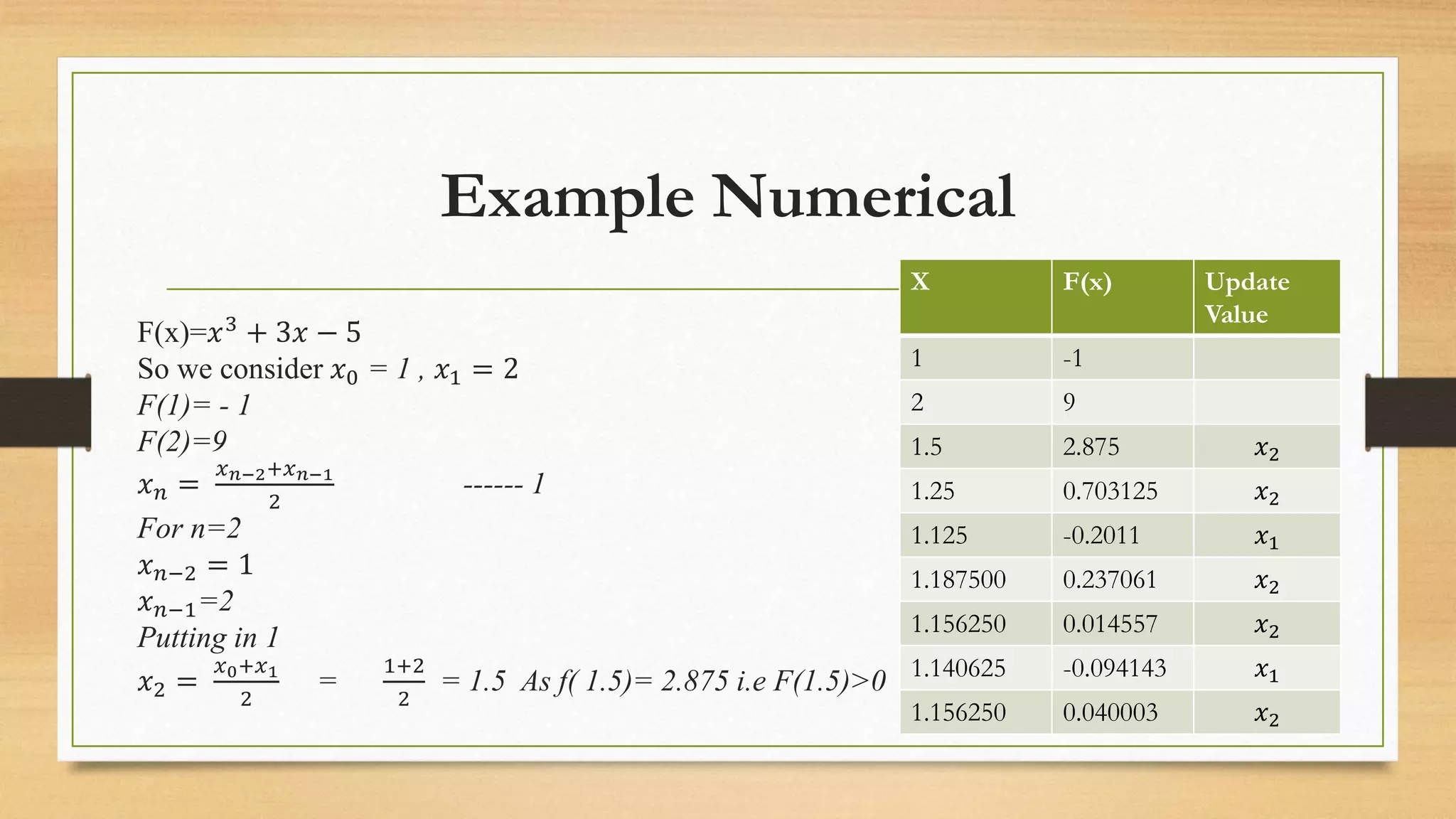
So replace 𝑥1with 𝑥2,
𝐼𝑛𝑡𝑒𝑟𝑣𝑎𝑙 𝑤𝑒 𝑐𝑜𝑛𝑠𝑖𝑑𝑒𝑟 𝑖𝑠
𝑥0 = 1 , 𝑥1 = 1.5 i.e [1,1.5]
𝑥2 =
𝑥0+𝑥1
2
=
1+1.5
2
= 1.25 As f(
1.25)= 2.875 i.e F(1.25)>0
𝑥3 =
𝑥1+𝑥2
2
=
1+1.25
2
= 1.125 As f(
1.125)= -0.2011 i.e F(1.125)<0
𝑥4 =
𝑥2+𝑥3
2
=
1.125+1.25
2
= 1.187500
As f(1.187500)= 0.237061
i.e. F(1.187500)>0
𝑥5 =
𝑥3+𝑥4
2
=
1.125+1.187500
2
= 1.156250
As f(1.156250)= 0.014557
i.e. F(1.156250)>0
X F(x) Up
dat
e
Val
ue
1 -1
2 9
1.5 2.875 𝑥2
1.25 0.703125 𝑥2
1.125 -0.2011 𝑥1
1.187500 0.237061 𝑥2
1.156250 0.014557 𝑥2
1.140625 -0.094143 𝑥1
1.156250 0.040003 𝑥2
Matlab Code
function_x=@(x) x.^3+3*x-5;
x1=1;
x2=2;
figure(1)
fplot(function_x,[x1 x2],'b-')
grid on
hold on
x_mid = (x1 + x2)/2;
iterate=1;
%fprintf('%f',abs(- 4))
%while
abs(myfunction(x_mid))>
0.01
while abs(x1 - x2) > 0.01 %or
you can change it to number
of iterations, it can be any
condition
if
(function_x(x2)*function_x(x
_mid))<0
x1=x_mid;
else
x2=x_mid;
end
x_mid = (x1+x2)/2;
%fprintf('The root of data is
%gn' , x_mid);
iterate=iterate+1;
fprintf('%d Approximation
Bracket is [%f,%f] gives
function value %f,%f
respectively and, mid value is
%fn',iterate,
x1,x2,function_x(x1),function
_x(x2),x_mid);
end
plot(x_mid,function_x(x_mid)
,'r')
fprintf('The root of data is
%fn and iteration is %dn' ,
x_mid,iterate);
Thank You 

Bisection

  • 1.
  • 2.
    Bisection Method WorkingRule •It begins with two values for x that bracket a root. It determines that they do in fact bracket a root because the function f(x) changes signs at these two x-values and, if f(x) is continuous. •The bisection method then successively divides the initial interval in half, finds in which half the root(s) must lie, and repeats with the endpoints of the smaller interval •Suppose, we wish to locate the root of an equation f (x) = 0 in an interval, say (x0, x1). Let f (x0) and f (x1) are of opposite signs, such that f (x0) f (x1) < 0.
  • 3.
  • 4.
    Formula Derivation 𝑥2= 𝑥0 +𝑥1 2 If f (x2) = 0, then x2 is the desired root of f (x) = 0. However, if f (x2) ≠ 0 then the root may be between x0 and x2 or x2 and x1. • As we know f(𝑥0)> 0 then, we can find which value to replace for next iteration by the following condition such as • If f(𝑥0)*f(𝑥2) < 0 then, 𝑥1= 𝑥2 else 𝑥0= 𝑥2 General form of this method is given by: 𝑥𝑛 = 𝑥𝑛−2 + 𝑥𝑛−1 2
  • 5.
  • 6.
    MERITS OF BISECTIONMETHOD 1. The iteration using bisection method always produces a root, since the method brackets the root between two values. 2. As iterations are conducted, the length of the interval gets halved. So one can guarantee the convergence in case of the solution of the equation. 3. Bisection method is simple to program in a computer.
  • 7.
    DEMERITS OF BISECTION METHOD 1.The convergence of bisection method is slow as it is simply based on halving the interval. 2. Cannot be applied over an interval where there is discontinuity. 3. Cannot be applied over an interval where the function takes always value of the same sign. 4. Method fails to determine complex roots (give only real roots) 5. If one of the initial guesses “𝑎0” or “𝑏0” is closer to the exact solution, it will take larger number of iterations to reach the root.
  • 8.
    Example Numerical F(x)=𝑥3 +3𝑥 − 5 So we consider 𝑥0 = 1 , 𝑥1 = 2 F(1)= - 1 F(2)=9 𝑥𝑛 = 𝑥𝑛−2+𝑥𝑛−1 2 ------ 1 For n=2 𝑥𝑛−2 = 1 𝑥𝑛−1=2 Putting in 1 𝑥2 = 𝑥0+𝑥1 2 = 1+2 2 = 1.5 As f( 1.5)= 2.875 i.e F(1.5)>0 X F(x) Update Value 1 -1 2 9 1.5 2.875 𝑥2 1.25 0.703125 𝑥2 1.125 -0.2011 𝑥1 1.187500 0.237061 𝑥2 1.156250 0.014557 𝑥2 1.140625 -0.094143 𝑥1 1.156250 0.040003 𝑥2
  • 9.
    Example Numerical So replace𝑥1with 𝑥2, 𝐼𝑛𝑡𝑒𝑟𝑣𝑎𝑙 𝑤𝑒 𝑐𝑜𝑛𝑠𝑖𝑑𝑒𝑟 𝑖𝑠 𝑥0 = 1 , 𝑥1 = 1.5 i.e [1,1.5] 𝑥2 = 𝑥0+𝑥1 2 = 1+1.5 2 = 1.25 As f( 1.25)= 2.875 i.e F(1.25)>0 𝑥3 = 𝑥1+𝑥2 2 = 1+1.25 2 = 1.125 As f( 1.125)= -0.2011 i.e F(1.125)<0 𝑥4 = 𝑥2+𝑥3 2 = 1.125+1.25 2 = 1.187500 As f(1.187500)= 0.237061 i.e. F(1.187500)>0 𝑥5 = 𝑥3+𝑥4 2 = 1.125+1.187500 2 = 1.156250 As f(1.156250)= 0.014557 i.e. F(1.156250)>0 X F(x) Up dat e Val ue 1 -1 2 9 1.5 2.875 𝑥2 1.25 0.703125 𝑥2 1.125 -0.2011 𝑥1 1.187500 0.237061 𝑥2 1.156250 0.014557 𝑥2 1.140625 -0.094143 𝑥1 1.156250 0.040003 𝑥2
  • 10.
    Matlab Code function_x=@(x) x.^3+3*x-5; x1=1; x2=2; figure(1) fplot(function_x,[x1x2],'b-') grid on hold on x_mid = (x1 + x2)/2; iterate=1; %fprintf('%f',abs(- 4)) %while abs(myfunction(x_mid))> 0.01 while abs(x1 - x2) > 0.01 %or you can change it to number of iterations, it can be any condition if (function_x(x2)*function_x(x _mid))<0 x1=x_mid; else x2=x_mid; end x_mid = (x1+x2)/2; %fprintf('The root of data is %gn' , x_mid); iterate=iterate+1; fprintf('%d Approximation Bracket is [%f,%f] gives function value %f,%f respectively and, mid value is %fn',iterate, x1,x2,function_x(x1),function _x(x2),x_mid); end plot(x_mid,function_x(x_mid) ,'r') fprintf('The root of data is %fn and iteration is %dn' , x_mid,iterate);
  • 11.