Download as PDF, PPTX

![Fractional Calculus
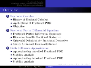
Fractional Partial Differential Equations
Finite Difference Approximation
Fractional Partial Differential Equations
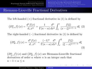
Riemann-Liouville Fractional Derivative
Gr¨unwald Definition for Fractional Derivative
Shifted Gr¨unwald Formula/Estimate
Shifted Gr¨unwald Formula/Estimate
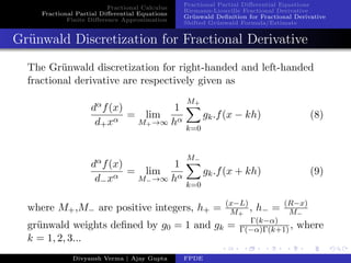
We define shifted Gr¨unwald formula as
dαf(x)
d+xα
= lim
M+→∞
1
hα
M+
k=0
gk.f[x − (k − 1)h] (10)
dαf(x)
d−xα
= lim
M−→∞
1
hα
M−
k=0
gk.f[x + (k − 1)h] (11)
which defines the following shifted Gr¨unwald estimates resp.
dαf(x)
d+xα
=
1
hα
M+
k=0
gk.f[x − (k − 1)h] + O(h) (12)
dαf(x)
d−xα
=
1
hα
M−
k=0
gk.f[x + (k − 1)h] + O(h) (13)
Divyansh Verma | Ajay Gupta FPDE](https://image.slidesharecdn.com/hzefwfbprnmwtm56ifvr-signature-aca8aa32a3e117212f8903b932b4ced8c00ff1f293d9ecd1445a7786e676bb86-poli-151231142320/85/FPDE-presentation-12-320.jpg)

![Fractional Calculus
Fractional Partial Differential Equations
Finite Difference Approximation
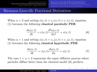
Approximating one-sided Fractional PDE
Stability Analysis
Approximating two-sided Fractional PDE
Stability Analysis
Stability Analysis
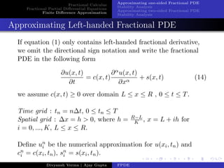
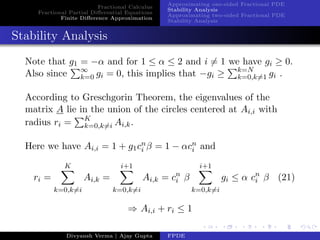
The difference equations defined by (19), together with the
Dirichlet boundary conditions, result in a linear system of
equations of the form
Un+1
= A Un
+ ∆t Sn
(20)
where Un
= [un
0 , un
1 , un
2 , ..., un
K]T , Sn
= [0, sn
0 , sn
1 , sn
2 , ..., sn
K−1, 0]T
and A is the matrix of coefficients, and is the sum of a lower
triangular matrix and a superdiagonal matrix. The matrix
entries Ai,j for i = 1, ..., K − 1 and j = 1, ..., K − 1
Ai,j = 0 , when j ≥ i + 2
= 1 + g1 β cn
i , when j = i
= gi−j+1 β cn
i , when otherwise
Divyansh Verma | Ajay Gupta FPDE](https://image.slidesharecdn.com/hzefwfbprnmwtm56ifvr-signature-aca8aa32a3e117212f8903b932b4ced8c00ff1f293d9ecd1445a7786e676bb86-poli-151231142320/85/FPDE-presentation-17-320.jpg)


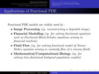
The document discusses fractional calculus and fractional partial differential equations (FPDEs). It provides background on fractional calculus, including its origins in the late 17th century. It then discusses applications of FPDEs in fields like image processing and finance. The objective is to numerically solve two-sided FPDEs using finite difference methods. It introduces the Riemann-Liouville definition of fractional derivatives and the Grünwald definition for approximating fractional derivatives. It then discusses approximating one-sided and two-sided FPDEs using finite differences and analyzes the stability of the resulting schemes.