NUMERICAL METHODS WITH MATLAB : bisection,mueller's,newton-raphson,false point,x=g(x)

Islamic Azad University
Qazvin Branch
Faculty of Industrial and Mechanics , Department of Mechanical
Engineering
Subject
Compare Some Algorithms for Solving Nonlinear Equation
Thesis Advisor
Dr.Marufi
By
Parham Sagharichi Ha

Assignment of Numerical Analysis Parham Sagharichi Ha
parhamsagharchi@gmail.com 1
Problem
The speed v of a Saturn V rocket in vertical flight near the surface of earth can
be approximated by
𝑣 = 𝑢 ln
𝑀0
𝑀0 − 𝑚̇ 𝑡
− 𝑔𝑡
𝑢 = 2510
𝑚
𝑠
= 𝑣𝑒𝑙𝑜𝑐𝑖𝑡𝑦 𝑜𝑓 𝑒𝑥ℎ𝑎𝑢𝑠𝑡 𝑟𝑒𝑙𝑎𝑡𝑖𝑣𝑒 𝑡𝑜 𝑡ℎ𝑒 𝑟𝑜𝑐𝑘𝑒𝑡
𝑀0 = 2.8 ∗ 106
𝑘𝑔 = 𝑚𝑎𝑠𝑠 𝑜𝑓 𝑟𝑜𝑐𝑘𝑒𝑡 𝑎𝑡 𝑙𝑖𝑓𝑡𝑜𝑓𝑓
𝑚̇ = 13.3 ∗ 103
𝑘𝑔
𝑠
= 𝑟𝑎𝑡𝑒 𝑜𝑓 𝑓𝑢𝑒𝑙 𝑐𝑜𝑛𝑠𝑢𝑚𝑝𝑡𝑖𝑜𝑛
𝑔 = 9.81
𝑚
𝑠2
= 𝑔𝑟𝑎𝑣𝑖𝑡𝑎𝑡𝑖𝑜𝑛𝑎𝑙 𝑎𝑐𝑐𝑒𝑙𝑒𝑟𝑎𝑡𝑖𝑜𝑛
𝑡 = 𝑡𝑖𝑚𝑒
Determine the time when the rocket reaches the speed of sound (335 m/s).
Solution
𝑢 𝑙𝑛
𝑀0
𝑀0 − 𝑚̇ 𝑡
− 𝑔𝑡 − 𝑣 = 0
Now we want to determine time in the above equation

Matlab
1) Bisection Method
Script :
clc
close all
clear all
%%
% Subject : Bisect Algorithm
% Author: Parham Sagharichi Ha Email :
parhamsagharchi@gmail.com
%%
%-------------------S------T------A------R------T------------
-------------%
global tolerance
tolerance = 1e-4; % for example : 1e-4 = 10^-4
u = 2510;
M0 = 2.8*10^6;
mdot = 13.3*10^3;
g = 9.81;
v = 335;
xlower = 0;
xupper = 100;
myfun = @(t)(u.*log(M0./(M0-mdot.*t))-g.*t-v);
[root,iflag] = fbisect(myfun,xlower,xupper);
switch iflag
case -2
disp('Initial range does not only contain one root')
otherwise
disp([' Root = ' num2str(root) ...
' found in ' num2str(iflag) ' iterations'])
end
%---------------F------I------N------I------S------H---------
-------------%

Function :
function [root,iflag] = fbisect(myfun,a,b)
if a>=b
disp(' attention b>a in [a b] ')
return
end
global tolerance
x = a:0.001:b;
y = feval(myfun,x);
fa = y(1);
fb = y(end);
ymax = max(y);
ymin = min(y);
figure
plot(x,y)
grid on
hold on
plot([a a],[ymin ymax])
plot([b b],[ymin ymax])
iflag = 0;
iterations = 0 ;
while (fa*fb<0) & (b-a)>tolerance
iterations = iterations + 1;
c = (a+b)/2;
fc = feval(myfun,c);
plot([c c],[ymin ymax])
pause
if fa*fc<0
b = c; fb = fc;
elseif fa*fc>0
a = c; fa = fc;
else
iflag = 1;
root = c
return
end
end
switch iterations
case 0
iflag = -2; root = NaN;
otherwise
iflag = iterations; root = c;
end

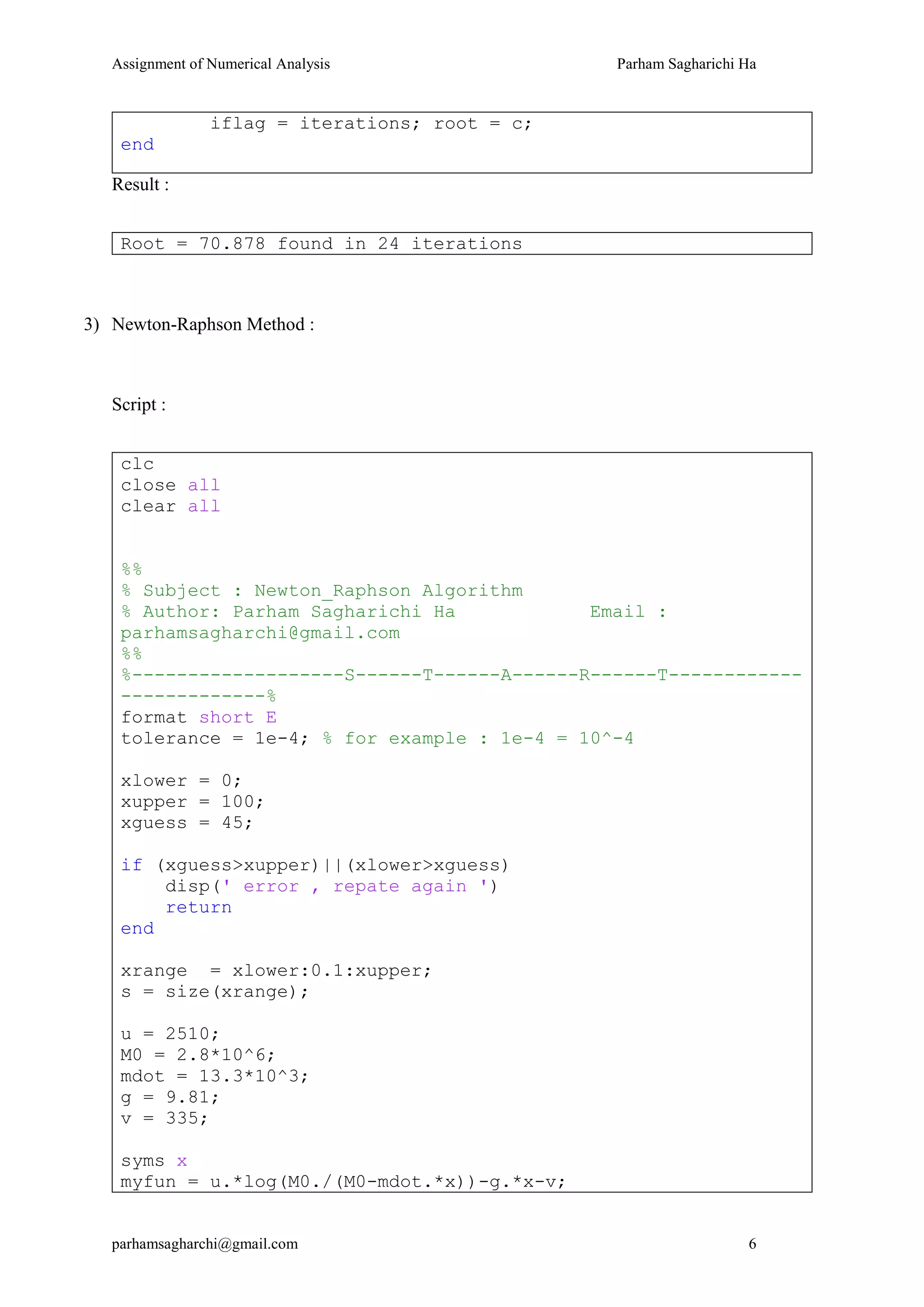
Result :
Root = 70.8779 found in 20 iterations
2) Linear Interpolation (False Position) Method :
Script :
clc
close all
clear all
%%
% Subject : False Postion Algorithm
%%
%-------------------S------T------A------R------T------------
-------------%
global tolerance
u = 2510;
M0 = 2.8*10^6;
mdot = 13.3*10^3;
g = 9.81;
v = 335;
xlower = 0;
xupper = 100;
[root,iflag] = finter(myfun,xlower,xupper);
switch iflag
case -2
disp('Initial range does not only contain one root')
otherwise
' found in ' num2str(iflag) ' iterations'])
end
%---------------F------I------N------I------S------H---------
-------------%

Function :
function [root,iflag] = finter(myfun,a,b)
if a>=b
disp(' attention b>a in [a b] ')
return
end
global tolerance
x = a:0.001:b;
y = feval(myfun,x);
fa = y(1);
fb = y(end);
ymax = max(y);
ymin = min(y);
figure
plot(x,y)
grid on
hold on
plot([a a],[ymin ymax])
plot([b b],[ymin ymax])
iflag = 0;
iterations = 0 ;
while (fa*fb<0) & (b-a)>tolerance
c = b - (fb)*(a-b)/(fa-fb);
fc = feval(myfun,c);
plot([c c],[ymin ymax])
pause
if fa*fc<0
b = c; fb = fc;
elseif fa*fc>0
a = c; fa = fc;
else
iflag = 1;
root = c
return
end
end
switch iterations
case 0
iflag = -2; root = NaN;
otherwise

iflag = iterations; root = c;
end
Result :
3) Newton-Raphson Method :
Script :
clc
close all
clear all
%%
% Subject : Newton_Raphson Algorithm
%%
%-------------------S------T------A------R------T------------
-------------%
format short E
xlower = 0;
xupper = 100;
xguess = 45;
if (xguess>xupper)||(xlower>xguess)
disp(' error , repate again ')
return
end
xrange = xlower:0.1:xupper;
s = size(xrange);
u = 2510;
M0 = 2.8*10^6;
mdot = 13.3*10^3;
g = 9.81;
v = 335;
syms x
myfun = u.*log(M0./(M0-mdot.*x))-g.*x-v;

u = 2510;
M0 = 2.8*10^6;
mdot = 13.3*10^3;
g = 9.81;
v = 335;
for i = 1:s(2);
y(i) = double(subs(myfun,[x],[xrange(i)]));
end
fa = y(1);
fb = y(end);
ymax = max(y);
ymin = min(y);
figure
plot(xrange,y)
grid on
hold on
plot([xlower xlower],[ymin ymax])
plot([xupper xupper],[ymin ymax])
plot([xlower xupper],[0 0])
iflag = 0;
iterations = 1 ;
f = double(subs(myfun,[x],xguess));
myfun_prime = jacobian(myfun,x);
fprime = double(subs(myfun_prime,[x],xguess));
xn = xguess;
xnew = xn - f/fprime;
plot([xn xn],[0 f])
pause
plot([xn xnew],[f 0])
while (abs(xnew-xn)>tolerance) & (iterations<30)
xn = xnew;
f = double(subs(myfun,[x],xn));
fprime = double(subs(myfun_prime,[x],xn));
xnew = xn - f/fprime;
root = xnew;
pause
plot([xn xn],[0 f])
pause
plot([xn xnew],[f 0])
end

switch iterations
case 30
disp(' Not root found ');
otherwise
' found in ' num2str(iterations) ' iterations
'])
end
%---------------F------I------N------I------S------H---------
-------------%
Result :
4) Mueller’s Method :
Script :
clc
close all
clear all
%%
% Subject : Mueller’s Algorithm
%%
%-------------------S------T------A------R------T------------
-------------%
u = 2510;
M0 = 2.8*10^6;
mdot = 13.3*10^3;
g = 9.81;
v = 335;
xlower = 0;
xupper = 100;

xguess = 45;
return
end
x = [xlower xguess xupper]';%[x2 x0 x1]
xe = xlower:0.1:xupper;
ye = feval(myfun,xe);
ymax = max(ye);
ymin = min(ye);
figure
plot(xe,ye)
grid on
hold on
rline = plot([xlower xlower],[ymin ymax]);
mline = plot([xguess xguess],[ymin ymax]);
fline = plot([xupper xupper],[ymin ymax]);
pause
iterations = 0;
while (true)
iterations = iterations +1;
y = feval(myfun,x);%[f2 f0 f1]
h1 = x(3)-x(2);
h2 = x(2)-x(1);
gamma = h2/h1;
c = y(2);
a = (gamma*y(3)-y(2)*(1+gamma)+y(1))/(gamma*h1^2*(1+gamma));
b = (y(3)-y(2)-a*h1^2)/h1;
if b>0
root = x(2)-(2*c)/(b+sqrt(b^2-4*a*c));
else
root = x(2)-(2*c)/(b-sqrt(b^2-4*a*c));
end
pause
rootline = plot([root root],[ymin ymax]);
if root>x(2)
x = [x(2) root x(3)];
else
x = [x(1) root x(2)];
end
pause
delete(rootline)
delete(rline)
delete(mline)
delete(fline)

rline = plot([x(1) x(1)],[ymin ymax]);
mline = plot([x(2) x(2)],[ymin ymax]);
fline = plot([x(3) x(3)],[ymin ymax]);
if (abs(feval(myfun,root))<(10^-8))&(iterations<30)
break
end
end
switch iterations
case 30
otherwise
' found in ' num2str(iterations) ' iterations
'])
end
Result :
5) 𝑥 = 𝑔(𝑥) Method :
𝑢 𝑙𝑛
𝑀0
𝑀0 − 𝑚̇ 𝑡
− 𝑔𝑡 − 𝑣 = 0
First Equation :
𝑡 =
𝑢
𝑔
𝑙𝑛
𝑀0
𝑀0 − 𝑚̇ 𝑡
−
𝑣
𝑔
Second Equation :
𝑡 =
𝑀0
𝑚̇
(
exp (
𝑔𝑡 + 𝑣
𝑢
) − 1
exp (
𝑔𝑡 + 𝑣
𝑢
)
)

Script :
clc
close all
clear all
%%
% Subject : x=g(x) Algorithm
%%
%-------------------S------T------A------R------T------------
-------------%
u = 2510;
M0 = 2.8*10^6;
mdot = 13.3*10^3;
g = 9.81;
v = 335;
xlower = 0;
xupper = 100;
xguess = 45;
return
end
myfun1 = @(t)((u/g).*log(M0./(M0-mdot.*t))-v/g);
myfun2 = @(t)((M0/mdot).*(exp((g.*t+v)/u)-
1)./exp((g.*t+v)/u));
xold1 = xguess;
xnew1 = feval(myfun1,xold1);
iterations1 = 0;
while (abs(xnew1-xold1)>tolerance)&(iterations1<30)
iterations1 = iterations1 + 1;
xold1 = xnew1;

end
root1 = xnew1(end);
switch iterations1
case 30
otherwise
disp([' Root1 = ' num2str(root1) ...
' found in ' num2str(iterations1) ' iterations1
'])
end
xold2 = xguess;
iterations2 = 0;
while (abs(xnew2-xold2)>tolerance)&(iterations2<30)
iterations2 = iterations2 + 1;
xold2 = xnew2;
end
root2 = xnew2(end)
switch iterations2
case 30
otherwise
disp([' Root2 = ' num2str(root2) ...
' found in ' num2str(iterations2) ' iterations2
'])
end
Result :
Not root found
root2 =
7.0878e+01
Root2 = 70.8779 found in 20 iterations2
References
Kiusalaas, J. (2009) Numerical Methods in Engineering with MATLAB®

NUMERICAL METHODS WITH MATLAB : bisection,mueller's,newton-raphson,false point,x=g(x)

Recommended

Recommended

More Related Content

What's hot

What's hot (20)

Viewers also liked

Viewers also liked (20)

Similar to NUMERICAL METHODS WITH MATLAB : bisection,mueller's,newton-raphson,false point,x=g(x)

Similar to NUMERICAL METHODS WITH MATLAB : bisection,mueller's,newton-raphson,false point,x=g(x) (20)

Recently uploaded

Recently uploaded (20)

NUMERICAL METHODS WITH MATLAB : bisection,mueller's,newton-raphson,false point,x=g(x)