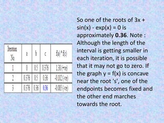
The False-Position Method is an iterative root-finding algorithm that improves upon the bisection method. It uses the slope of a line between two points to estimate a new root, rather than always bisecting the interval. Given an initial interval where the function changes sign, it calculates a new x-value at the intersection of the x-axis and a line through two existing points. It then chooses a new interval based on where the function changes sign again. The method is similar to bisection but uses a different formula to calculate the new estimate. An example finds a root of 3x + sin(x) - exp(x) = 0 between 0 and 0.5, converging to a solution of approximately 0.
Here we focuses on Fixed-Point Iterative Technique for solving nonlinear Equations in Numerical Analysis. It is one of the opened-iterative techniques for finding roots called Fixed-Point of Non-linear Equations.
In numerical analysis, Newton's method (also known as the Newton–Raphson method), named after Isaac Newton and Joseph Raphson, is a method for finding successively better approximations to the roots (or zeroes) of a real-valued function.
The method starts with a function f defined over the real numbers x, the function's derivative f', and an initial guess x0 for a root of the function f.
This lecture contains Newton Raphson Method working rule, Graphical representation, Example, Pros and cons of this method and a Matlab Code.
Explanation is available here: https://www.youtube.com/watch?v=NmwwcfyvHVg&lc=UgwqFcZZrXScgYBZPcV4AaABAg
Computer Oriented Numerical Analysis
What is interpolation?
Many times, data is given only at discrete points such as .
So, how then does one find the value of y at any other value of x ?
Well, a continuous function f(x) may be used to represent the data values with f(x) passing through the points (Figure 1). Then one can find the value of y at any other value of x .
This is called interpolation
Newton’s Divided Difference Formula:
To illustrate this method, linear and quadratic interpolation is presented first.
Then, the general form of Newton’s divided difference polynomial method is presented.
Algorithms Lecture 3: Analysis of Algorithms IIMohamed Loey
We will discuss the following: Maximum Pairwise Product, Fibonacci, Greatest Common Divisors, Naive algorithm is too slow. The Efficient algorithm is much better. Finding the correct algorithm requires knowing something interesting about the problem
This slides contains assymptotic notations, recurrence relation like subtitution method, iteration method, master method and recursion tree method and sorting algorithms like merge sort, quick sort, heap sort, counting sort, radix sort and bucket sort.
Psychology: Motivation,Types of Motivation & Theories of MotivationPriyanka Nain
This presentation is basically about Motivation,categories & types of Motivation. It also consists of two theories of Motivation- McClelland's Theory of Needs and Maslow's Theory of Self Actualization.
APPROXIMATIONS; LINEAR PROGRAMMING;NON- LINEAR FUNCTIONS; PROJECT MANAGEMENT WITH PERT/CPM; DECISION THEORY; THEORY OF GAMES; INVENTORY MODELLING; QUEUING THEORY
This 10 hours class is intended to give students the basis to empirically solve statistical problems. Talk 1 serves as an introduction to the statistical software R, and presents how to calculate basic measures such as mean, variance, correlation and gini index. Talk 2 shows how the central limit theorem and the law of the large numbers work empirically. Talk 3 presents the point estimate, the confidence interval and the hypothesis test for the most important parameters. Talk 4 introduces to the linear regression model and Talk 5 to the bootstrap world. Talk 5 also presents an easy example of a markov chains.
All the talks are supported by script codes, in R language.
A polynomial interpolation algorithm is developed using the Newton's divided-difference interpolating polynomials. The definition of monotony of a function is then used to define the least degree of the polynomial to make efficient and consistent the interpolation in the discrete given function. The relation between the order of monotony of a particular function and the degree of the interpolating polynomial is justified, analyzing the relation between the derivatives of such function and the truncation error expression. In this algorithm there is not matter about the number and the arrangement of the data points, neither if the points are regularly spaced or not. The algorithm thus defined can be used to make interpolations in functions of one and several dependent variables. The algoritm automatically select the data points nearest to the point where an interpolation is desired, following the criterion of symmetry. Indirectly, the algorithm also select the number of data points, which is a unity higher than the order of the used polynomial, following the criterion of monotony. Finally, the complete algoritm is presented and subroutines in fortran code is exposed as an addendum. Notice that there is not the degree of the interpolating polynomial within the arguments of such subroutines.
1 Part 2 Systems of Equations Which Do Not Have A Uni.docxeugeniadean34240
1
Part 2: Systems of Equations Which Do Not Have A Unique
Solution
On the previous pages we learned how to solve systems of equations using Gaussian
elimination. In each of the examples and exercises of part 1(except for exercise 1 parts d and e)
the systems of equations had a unique solution. That is, a single value for each of the variables.
In example 3 we found the solution to be 7 23 3, . This means that the graphs of the two lines in
example 3 intersect at this unique point. In 2-space, the xy-plane, we have the geometric bonus
of being able to draw a picture of the solutions to a system of two equations two unknowns.
Clearly, if we were asked to draw the graphs of two lines in the xy-plane we have 3 basic
choices/cases:
1. Draw the two lines so they intersect. This point of intersection can only happen once for
a given pair of lines. That is, the two lines intersect in a unique point. There is a unique
common solution to the system of equations. Discussed in part 1.
2. Draw the two lines so that one is on "top of" the other. In this case there are an infinite
number of common points, an infinite number of solutions to the given system. Discussed
in part 2.
3. Draw two parallel lines. In this case there are no points common to both lines. There is
no solution to the system of equations that describe the lines. Discussed in part 2.
The 3 cases above apply to any system of equations.
Theorem 1. For any system of m equations with n unknowns (m < n) one of the following cases
applies:
1. There is a unique solution to the system.
2. There is an infinite number of solutions to the system.
3. There are no solutions to the system.
Again, in this section of the notes we will illustrate cases 2 and 3. To solve systems of
equations where these cases apply we use the matrix procedure developed previously.
Example 6. Solve the system
x + 2y = 1
2x + 4y = 2
2
It is probably already clear to the reader that the second equation is really the first in
disguise. (Simply divide both sides of the second equation by 2 to obtain the first). So if we
were to draw the graph of both we would obtain the same line, hence have an infinite number of
points common to both lines, an infinite number of solutions. However it would be helpful in
solving other systems where the solutions may not be so apparent to do the problem
algebraically, using matrices. The matrix of the system with its simplification follows. Recall,
we try to express the matrix
1 2 1
2 4 2
in the form 1
2
1 0
0 1
b
b
from which we can read off the
solution. However after one step we note that
1 2 1
2 4 2
1 22 R R
1 2 1
0 0 0
. It should be clear to the reader that no matter what further
elementary row operations we perform on the matrix
1 2 1
0 0 0
we cannot change it to the form
we hoped for, namel.
2. Introduction
The poor convergence of the bisection
method as well as its poor adaptability
to higher dimensions motivate the use
of better techniques. One such
method is the Method of False
Position.
3. Methodology
we start with an initial interval [x1,x2], and we
assume that the function changes sign only once
in this interval. Now we find an x3 in this
interval, which is given by the intersection of the
x axis and the straight line passing through
(x1,f(x1)) and (x2,f(x2)). It is easy to verify that
x3 is given by
4. Methodology
Now, we choose the new
interval from the two choices
[x1,x3] or [x3,x2] depending on in
which interval the function
changes sign.
5. Note
The False-Position and Bisection
algorithms are
quite similar. The only difference is
the formula used to
calculate the new estimate of the
root x3
7. Numerical Example
Find a root of 3x + sin(x) - exp(x) =0. The
graph of this equation is given in the
figure.
From this it's clear that there is a
root between 0
and 0.5 and also
another root between 1.5 and
2.0. Now let us consider the function f
(x) in the
interval [0, 0.5] where f (0) * f (0.5) is
less than
zero and use the regula-falsi scheme to
obtain the
zero of f (x) = 0.
8. So one of the roots of 3x +
sin(x) - exp(x) = 0 is
approximately 0.36. Note :
Although the length of the
interval is getting smaller in
each iteration, it is possible
that it may not go to zero. If
the graph y = f(x) is concave
near the root 's', one of the
endpoints becomes fixed and
the other end marches
towards the root.