Downloaded 211 times

![ters II
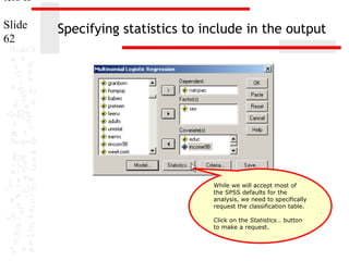
Relationship of individual independent
variables and the dependent variable
Slide
21
Likelihood Ratio Tests
Effect
Intercept
AGE
EDUC
POLVIEWS
SEX
-2 Log
Likelihood of
Reduced
Model
327.463a
333.440
329.606
334.636
338.985
Chi-Square
.000
5.976
2.143
7.173
11.521
df
Sig.
0
2
2
2
2
.
.050
.343
.028
.003
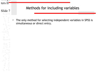
The chi-square statistic is the difference in -2 log-likelihoods
Parameter Estimates
between the final model and a reduced model. The reduced model
is formed by omitting an effect from the final model. The null
hypothesis is that all parameters of that effect are 0.
a.
a
NATCHLD
B
Std. Error
Wald
df
This reduced model is equivalent to the final2.233 because
model
TOO LITTLE
Intercept
8.434
14.261
1
omitting the effect does not increase the degrees of freedom.
AGE
-.023
.017
1.756
1
EDUC
-.066
.102
.414
1
POLVIEWS
-.575
.251
5.234
1
[SEX=1]
-2.167
.805
7.242
1
b
[SEX=2]
0
.
.
0
ABOUT RIGHT Intercept
4.485
2.255
3.955
1
AGE
-.001
.018
.003
1
EDUC
.011
.104
.011
1
POLVIEWS
-.397
.257
2.375
1
[SEX=1]
-1.606
.824
3.800
1
b
[SEX=2]
0
.
.
0
a. The reference category is: TOO MUCH.
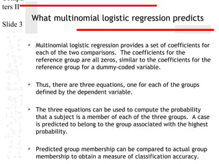
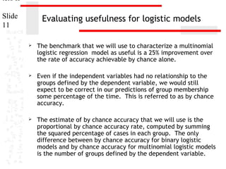
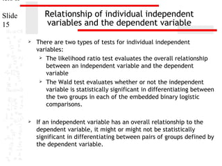
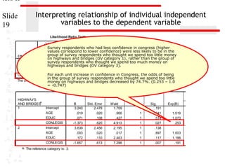
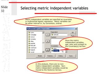
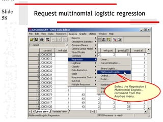
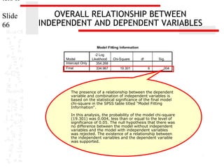
In this example, there is
a statistically significant
relationship between SEX
and the dependent
variable, spending on
childcare assistance.
As well, SEX plays a
statistically significant role
in differentiating 95% Confidence Interval
the TOO
LITTLE group from the TOO
Exp(B)
MUCH Exp(B)
(reference) group.
Sig.
Lower Bound
Upper Bo
(0.007 < 0.5)
.000
.185
.977
.944
.520
.936
.766
.022
.563
.344
.007
.115
.024
.
.
.
However, SEX does not
.047differentiate the ABOUT
.955RIGHT .999
.965
group from the
TOO MUCH (reference)
.916
1.011
.824
group.(0.51 > 0.5)
.123
.673
.406
.051
.201
.040
.
.
.
1.
1.
.
.
1.
1.
1.
1.](https://image.slidesharecdn.com/multinomiallogisticregressionbasicrelationships-140123080904-phpapp02/85/Multinomial-logisticregression-basicrelationships-21-320.jpg)
![ters II
Slide
22
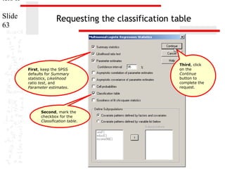
Interpreting relationship of individual independent
variables and the dependent variable
Likelihood Ratio Tests
Effect
Intercept
AGE
EDUC
POLVIEWS
SEX
-2 Log
Likelihood of
Reduced
Model
Chi-Square
df
Sig.
327.463a
.000
0
.
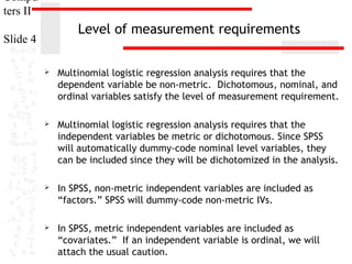
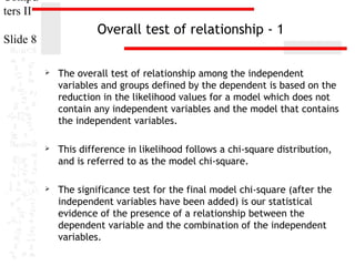
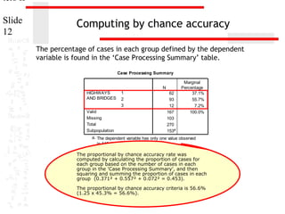
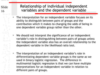
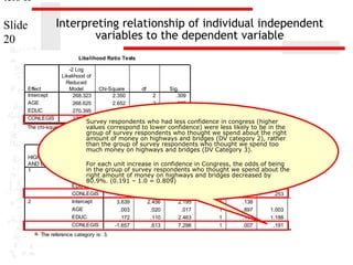
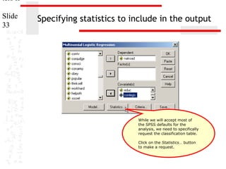
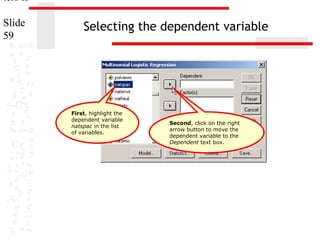
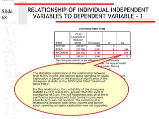
Survey respondents who were2 male (code 1 for sex) were less likely
333.440
5.976
.050
to 329.606
be in the group of survey respondents who thought we spend too
2.143
2
.343
little money on childcare assistance (DV category 1), rather than the
334.636
2
.028
group of survey 7.173
respondents who thought we spend too much
money on childcare assistance (DV category 3).
338.985
11.521
2
.003
The chi-square statistic is the difference in -2 log-likelihoods
Survey respondents who were male were 88.5% less likely (0.115 –
Parameter Estimates
between the final model and a reduced model. The reduced model
1.0 = -0.885) to be in the group of survey respondents who thought
is formed by omittingspend too little final model. The null
we an effect from the money on childcare assistance.
hypothesis is that all parameters of that effect are 0.
a.
a
NATCHLD
B
Std. Error
Wald
df
Sig.
Exp(B)
This reduced model is equivalent to the final2.233 because
model
TOO LITTLE
Intercept
8.434
14.261
1
.000
omitting the effect does not increase the degrees of freedom.
AGE
-.023
.017
1.756
1
.185
.977
EDUC
-.066
.102
.414
1
.520
.936
POLVIEWS
-.575
.251
5.234
1
.022
.563
[SEX=1]
-2.167
.805
7.242
1
.007
.115
b
[SEX=2]
0
.
.
0
.
.
ABOUT RIGHT Intercept
4.485
2.255
3.955
1
.047
AGE
-.001
.018
.003
1
.955
.999
EDUC
.011
.104
.011
1
.916
1.011
POLVIEWS
-.397
.257
2.375
1
.123
.673
[SEX=1]
-1.606
.824
3.800
1
.051
.201
b
[SEX=2]
0
.
.
0
.
.
a. The reference category is: TOO MUCH.
95% Confidence Interval
Exp(B)
Lower Bound
Upper Bo
.944
.766
.344
.024
.
1.
1.
.
.
.965
.824
.406
.040
.
1.
1.
1.
1.](https://image.slidesharecdn.com/multinomiallogisticregressionbasicrelationships-140123080904-phpapp02/85/Multinomial-logisticregression-basicrelationships-22-320.jpg)
![ters II
Slide
24
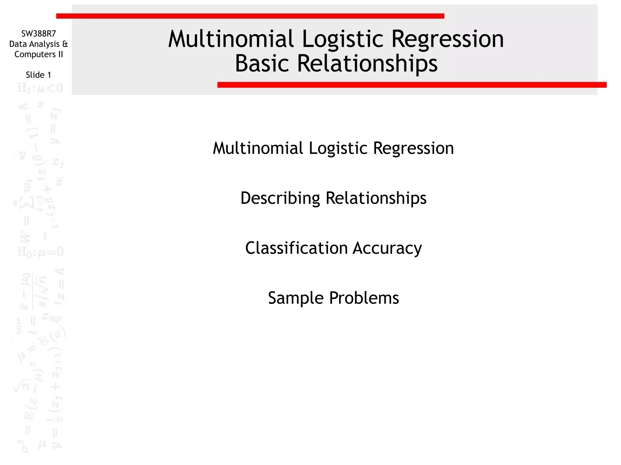
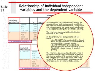
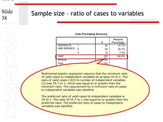
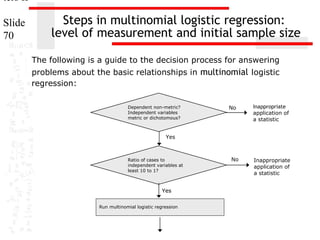
Problem 1
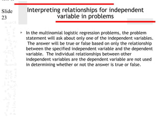
11. In the dataset GSS2000, is the following statement true, false, or an incorrect application
of a statistic? Assume that there is no problem with missing data, outliers, or influential cases,
and that the validation analysis will confirm the generalizability of the results. Use a level of
significance of 0.05 for evaluating the statistical relationships.
The variables "age" [age], "highest year of school completed" [educ] and "confidence in
Congress" [conlegis] were useful predictors for distinguishing between groups based on
responses to "opinion about spending on highways and bridges" [natroad]. These predictors
differentiate survey respondents who thought we spend too little money on highways and
bridges from survey respondents who thought we spend too much money on highways and
bridges and survey respondents who thought we spend about the right amount of money on
highways and bridges from survey respondents who thought we spend too much money on
highways and bridges.
Among this set of predictors, confidence in Congress was helpful in distinguishing among the
groups defined by responses to opinion about spending on highways and bridges. Survey
respondents who had less confidence in congress were less likely to be in the group of survey
respondents who thought we spend too little money on highways and bridges, rather than the
group of survey respondents who thought we spend too much money on highways and bridges.
For each unit increase in confidence in Congress, the odds of being in the group of survey
respondents who thought we spend too little money on highways and bridges decreased by
74.7%. Survey respondents who had less confidence in congress were less likely to be in the
group of survey respondents who thought we spend about the right amount of money on
highways and bridges, rather than the group of survey respondents who thought we spend too
much money on highways and bridges. For each unit increase in confidence in Congress, the
odds of being in the group of survey respondents who thought we spend about the right amount
of money on highways and bridges decreased by 80.9%.
1.
2.
3.
4.
True
True with caution
False
Inappropriate application of a statistic](https://image.slidesharecdn.com/multinomiallogisticregressionbasicrelationships-140123080904-phpapp02/85/Multinomial-logisticregression-basicrelationships-24-320.jpg)
![ters II
Slide
25
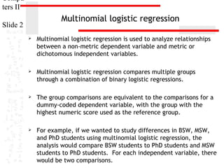
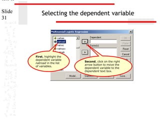
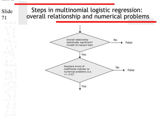
Dissecting problem 1 - 1
11. In the dataset GSS2000, is the following statement true, false, or an incorrect application
of a statistic? Assume that there is no problem with missing data, outliers, or influential cases,
and that the validation analysis will confirm the generalizability of the results. Use a level of
significance of 0.05 for evaluating the statistical relationships.
The variables "age" [age], "highest year of school completed" [educ] and "confidence in
Congress" [conlegis] were useful predictors for distinguishing between groups based on
responses to "opinion about spending on highways and bridges" [natroad]. These predictors
differentiate survey respondents who For thesewe spend too little money on highways and
thought problems, we will
bridges from survey respondents who assume that spend is nomuch money on highways and
thought we there too problem
bridges and survey respondents who thought we spend about the right amount of money on
with missing data, outliers, or
highways and bridges from survey respondents who thought wethe
influential cases, and that spend too much money on
highways and bridges.
validation analysis will confirm
the generalizability of the
Among this set of predictors, confidence in Congress was helpful in distinguishing among the
results
groups defined by responses to opinion about spending on highways and bridges. Survey
respondents who had less confidence in congress were less likely to be in the group of survey
In this money we are told and
respondents who thought we spend too littleproblem,on highways to bridges, rather than the
use we spend too much
group of survey respondents who thought 0.05 as alpha for the money on highways and bridges.
For each unit increase in confidence in Congress, logistic regression. in the group of survey
multinomial the odds of being
respondents who thought we spend too little money on highways and bridges decreased by
74.7%. Survey respondents who had less confidence in congress were less likely to be in the
group of survey respondents who thought we spend about the right amount of money on
highways and bridges, rather than the group of survey respondents who thought we spend too
much money on highways and bridges. For each unit increase in confidence in Congress, the
odds of being in the group of survey respondents who thought we spend about the right amount
of money on highways and bridges decreased by 80.9%.
1.
2.
3.
4.
True
True with caution
False
Inappropriate application of a statistic](https://image.slidesharecdn.com/multinomiallogisticregressionbasicrelationships-140123080904-phpapp02/85/Multinomial-logisticregression-basicrelationships-25-320.jpg)
![ters II
Slide
26
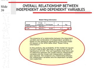
Dissecting problem 1 - 2
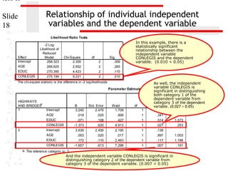
The variables listed first in the problem
statement are the independent variables
(IVs): "age" [age], "highest year of school
11. In the dataset GSS2000,"confidence in
completed" [educ] and is the following statement true, false, or an incorrect application
of a statistic? Assume that there is no problem with missing data, outliers, or influential cases,
Congress" [conlegis].
and that the validation analysis will confirm the generalizability of the results. Use a level of
significance of 0.05 for evaluating the statistical relationships.
The variables "age" [age], "highest year of school completed" [educ] and "confidence in
Congress" [conlegis] were useful predictors for distinguishing between groups based on
responses to "opinion about spending on highways and bridges" [natroad]. These predictors
differentiate survey respondents who thought we spend too little money on highways and
bridges from survey respondents who thought we spend too much money on highways and
bridges and survey respondents who thought we spend about the right amount of money on
highways and bridges from survey respondents who thought we spend too much money on
The variable used to define
highways and bridges.the dependent
groups is
variable (DV): "opinion about
Among this set of predictors, confidence in Congress was helpful in distinguishing among the
spending on highways and
groups defined by responses to opinion about spending on highways and bridges. Survey
respondents bridges" [natroad].
who had less confidence in congress were less likely to be in the group of survey
respondents who thought we spend too little money on highways and bridges, rather than the
group of survey respondents who thought we spend too much money on highways and bridges.
For each unit increase in confidence in Congress, the odds of being in the group of survey
respondents who thought we spend too little moneySPSS only supports direct or
on highways and bridges decreased by
simultaneous entry of independent in the
74.7%. Survey respondents who had less confidence in congress were less likely to be
group of survey respondents who thought we spend variables in multinomial logistic
about the right amount of money on
regression, so we have no choice of
highways and bridges, rather than the group of survey respondents who thought we spend too
much money on highways and bridges. For each unitmethod for entering variables.
increase in confidence in Congress, the
odds of being in the group of survey respondents who thought we spend about the right amount
of money on highways and bridges decreased by 80.9%.](https://image.slidesharecdn.com/multinomiallogisticregressionbasicrelationships-140123080904-phpapp02/85/Multinomial-logisticregression-basicrelationships-26-320.jpg)
![ters II
Slide
27
Dissecting problem 1 - 3
SPSS multinomial logistic regression models the relationship by
comparing each of the groups defined by the dependent variable to the
group with the highest code value.
11. In the dataset GSS2000, opinionfollowing statement true, false, or an incorrect application
The responses to is the about spending on highways and bridges were:
of a statistic? Assume that there is no problem with missing data, outliers, or influential cases,
and that the validation analysis will confirm the= Too much.
generalizability of the results. Use a level of
1= Too little, 2 = About right, and 3
significance of 0.05 for evaluating the statistical relationships.
The variables "age" [age], "highest year of school completed" [educ] and "confidence in
Congress" [conlegis] were useful predictors for distinguishing between groups based on
responses to "opinion about spending on highways and bridges" [natroad]. These predictors
differentiate survey respondents who thought we spend too little money on highways and
bridges from survey respondents who thought we spend too much money on highways and
bridges and survey respondents who thought we spend about the right amount of money on
highways and bridges from survey respondents who thought we spend too much money on
highways and bridges.
Among this set of predictors, confidence in Congress was helpful in distinguishing among the
groups defined by responses to opinion about spending on highways and bridges. Survey
respondents who had less confidence in congress were less likely to be in the group of survey
respondents who The analysis spend too in two money on highways and bridges, rather than the
thought we will result little comparisons:
group of survey respondents who thought we spend too spend too little money
• survey respondents who thought we much money on highways and bridges.
For each unit increase in confidence in Congress, the odds of being in the group of survey
versus survey respondents who thought we spend too much
respondents who thought we spend too and bridges on highways and bridges decreased by
money on highways little money
74.7%. Survey respondents respondents who thought wecongress were less likely to be in the
• survey who had less confidence in spend about the right
group of survey respondentsof money versus survey respondents whoamount of money on
who thought we spend about the right thought we
amount
highways and bridges, rather than the group of survey respondents who thought we spend too
spend too bridges. For on highways and bridges.
much money on highways and much money each unit increase in confidence in Congress, the
odds of being in the group of survey respondents who thought we spend about the right amount
of money on highways and bridges decreased by 80.9%.](https://image.slidesharecdn.com/multinomiallogisticregressionbasicrelationships-140123080904-phpapp02/85/Multinomial-logisticregression-basicrelationships-27-320.jpg)
![ters II
Slide
28
Dissecting problem 1 - 4
Each problem includes a statement about the relationship between
one independent variable and the dependent variable. The answer
to the problem is based on the stated relationship, ignoring the
The variablesrelationships between the other independent variables and the
"age" [age], "highest year of school completed" [educ] and "confidence in
dependent variable.
Congress" [conlegis] were useful predictors for distinguishing between groups based on
responses to "opinion about spending on highways and bridges" [natroad]. These predictors
differentiate This problem identifies a difference forspendof the comparisons highways and
survey respondents who thought we both too little money on
bridges from among respondents who thought we spend too much money on highways and
survey groups modeled by the multinomial logistic regression.
bridges and survey respondents who thought we spend about the right amount of money on
highways and bridges from survey respondents who thought we spend too much money on
highways and bridges.
Among this set of predictors, confidence in Congress was helpful in distinguishing among the
groups defined by responses to opinion about spending on highways and bridges. Survey
respondents who had less confidence in congress were less likely to be in the group of
survey respondents who thought we spend too little money on highways and bridges, rather
than the group of survey respondents who thought we spend too much money on highways
and bridges. For each unit increase in confidence in Congress, the odds of being in the
group of survey respondents who thought we spend too little money on highways and
bridges decreased by 74.7%. Survey respondents who had less confidence in congress were
less likely to be in the group of survey respondents who thought we spend about the right
amount of money on highways and bridges, rather than the group of survey respondents
who thought we spend too much money on highways and bridges. For each unit increase in
confidence in Congress, the odds of being in the group of survey respondents who thought
we spend about the right amount of money on highways and bridges decreased by 80.9%.](https://image.slidesharecdn.com/multinomiallogisticregressionbasicrelationships-140123080904-phpapp02/85/Multinomial-logisticregression-basicrelationships-28-320.jpg)
![ters II
Slide
29
Dissecting problem 1 - 5
11. In the dataset GSS2000, is the following statement true, false, or an incorrect application
of a statistic? Assume that there is no problem with missing data, outliers, or influential cases,
and that the validation analysis will confirm the generalizability of the results. Use a level of
significance of 0.05 for evaluating the statistical relationships.
The variables "age" [age], "highest year of school completed" [educ] and "confidence in
Congress" [conlegis] were useful predictors for distinguishing between groups based on
responses to "opinion about spending on highways and bridges" [natroad]. These predictors
differentiate survey respondents who thought we spend too little money on highways and
bridges from survey respondents who thought we spend too much money on highways and
bridges and survey respondents who thought we spend about the right amount of money on
highways and bridges from survey respondents who thought we spend too much money on
highways and bridges.
Among this set of predictors, confidence in Congress was helpful in distinguishing among the
groups defined by responses to opinion about spending on highways and bridges. Survey
respondents who had less confidence in congress were less likely to be in the group of survey
respondents who thought we spend too little money on highways and bridges, rather than the
group of survey respondents who thought we spend too much money on highways and bridges.
In order for the multinomial logistic regression
For each unit increase in confidence in Congress, the odds of being in the group of survey
question to be on highways and bridges decreased
respondents who thought we spend too little money true, the overall relationship must by
be statistically significant, were less be no
74.7%. Survey respondents who had less confidence in congress there mustlikely to be in the
evidence of numerical problems, the classification
group of survey respondents who thought we spend about the right amount of money on
highways and bridges, rather than the accuracy rate must be substantiallythought we spend too
group of survey respondents who better than
much money on highways and bridges.couldeach unit increase in confidence in Congress, the
For be obtained by chance alone, and the
odds of being in the group of survey respondents who thought we spendbe statistically amount
stated individual relationship must about the right
of money on highways and bridges decreased by and interpreted correctly.
significant 80.9%.](https://image.slidesharecdn.com/multinomiallogisticregressionbasicrelationships-140123080904-phpapp02/85/Multinomial-logisticregression-basicrelationships-29-320.jpg)

![ters II
Slide
36
LEVEL OF MEASUREMENT - 1
11. In the dataset GSS2000, is the following statement true, false, or an incorrect application
of a statistic? Assume that there is no problem with missing data, outliers, or influential cases,
and that the validation analysis will confirm the generalizability of the results. Use a level of
significance of 0.05 for evaluating the statistical relationships.
The variables "age" [age], "highest year of school completed" [educ] and "confidence in
Congress" [conlegis] were useful predictors for distinguishing between groups based on
responses to "opinion about spending on highways and bridges" [natroad]. These predictors
differentiate survey respondents who thought we spend too little money on highways and
bridges from survey respondents who thought we spend too much money on highways and
bridges and survey respondents who thought we spend about the right amount of money on
highways and bridges from survey respondents who thought we spend too much money on
highways and bridges.
Among this set of predictors, confidence in Congress was helpful in distinguishing among the
groups defined by responses to opinion about spending on highways and bridges. Survey
respondents who had less confidence in congressrequires that the to be in the group of survey
Multinomial logistic regression were less likely
respondents who thought we spend too little money andhighways and bridges, rather than the
dependent variable be non-metric on the
group of survey respondents who thought we spend too much money on highways and bridges.
independent variables be metric or dichotomous.
For each unit increase in confidence in Congress, the odds of being in the group of survey
respondents who thought we spend too little money on highways and bridges decreased by
"Opinion about spending on highways and
bridges" [natroad] is confidence in congress were less likely to be in the
74.7%. Survey respondents who had lessordinal, satisfying the nonmetric level of thought we spend about the the
group of survey respondents who measurement requirement forright amount of money on
dependent variable.
highways and bridges, rather than the group of survey respondents who thought we spend too
much money on highways and bridges. For each unit increase in confidence in Congress, the
It contains three respondents who thought we
odds of being in the group of surveycategories: survey respondents spend about the right amount
who thought we spend too
of money on highways and bridges decreased little money, about
the right amount of money, by 80.9%.
and too much
money on highways and bridges.
1. True
2. True with caution](https://image.slidesharecdn.com/multinomiallogisticregressionbasicrelationships-140123080904-phpapp02/85/Multinomial-logisticregression-basicrelationships-36-320.jpg)
![ters II
Slide
37
LEVEL OF MEASUREMENT - 2
"Age" [age] and "highest year of
school completed" [educ] are interval,
11. satisfying the metric or dichotomous
In the dataset GSS2000, is the following statement true, false, or an incorrect application
of alevel of measurement requirement for
statistic? Assume that there is no problem with missing data, outliers, or influential cases,
independent variables.
and that the validation analysis will confirm the generalizability of the results. Use a level of
significance of 0.05 for evaluating the statistical relationships.
The variables "age" [age], "highest year of school completed" [educ] and "confidence in
Congress" [conlegis] were useful predictors for distinguishing between groups based on
responses to "opinion about spending on highways and bridges" [natroad]. These predictors
differentiate survey respondents who thought we spend too little money on highways and
bridges from survey respondents who thought we spend too much money on highways and
bridges and survey respondents who thought we spend about the right amount of money on
highways and bridges from survey respondents who thought we spend too much money on
"Confidence in Congress" [conlegis] is ordinal,
highways and bridges. satisfying the metric or dichotomous level of
measurement requirement for independent
variables. If we follow the convention of treating
Among this set of predictors, confidence in Congress was helpfulthe distinguishing among the
ordinal level variables as metric variables, in level
groups defined by responses to opinion about spending on highways is bridges. Survey
of measurement requirement for the analysis and
respondents who had less confidence in congress analysts do not agree in the group of survey
satisfied. Since some data were less likely to be
with this convention, a note of caution should be
respondents who thought we spend too little money on highways and bridges, rather than the
included in our interpretation.
group of survey respondents who thought we spend too much money on highways and bridges.
For each unit increase in confidence in Congress, the odds of being in the group of survey
respondents who thought we spend too little money on highways and bridges decreased by
74.7%. Survey respondents who had less confidence in congress were less likely to be in the
group of survey respondents who thought we spend about the right amount of money on
highways and bridges, rather than the group of survey respondents who thought we spend too
much money on highways and bridges. For each unit increase in confidence in Congress, the
odds of being in the group of survey respondents who thought we spend about the right amount
of money on highways and bridges decreased by 80.9%.](https://image.slidesharecdn.com/multinomiallogisticregressionbasicrelationships-140123080904-phpapp02/85/Multinomial-logisticregression-basicrelationships-37-320.jpg)
![ters II
RELATIONSHIP OF INDIVIDUAL INDEPENDENT
VARIABLES TO DEPENDENT VARIABLE - 2
Slide
42
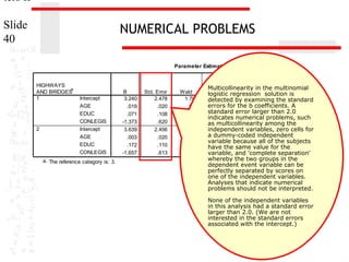
Parameter Estimates
HIGHWAYS
a
AND BRIDGES
1
2
Intercept
AGE
EDUC
CONLEGIS
Intercept
AGE
EDUC
CONLEGIS
B
3.240
.019
.071
-1.373
3.639
.003
.172
-1.657
Std. Error
2.478
.020
.108
.620
2.456
.020
.110
.613
Wald
1.709
.906
.427
4.913
2.195
.017
2.463
7.298
df
1
1
1
1
1
1
1
1
Sig.
.191
.341
.514
.027
.138
.897
.117
.007
a. The reference category is: 3.
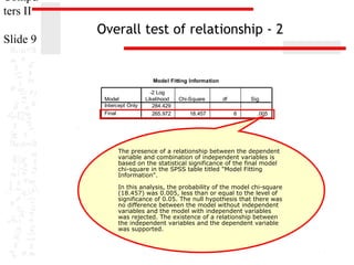
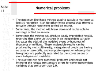
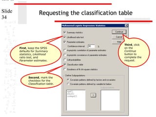
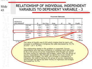
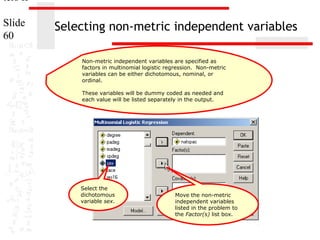
In the comparison of survey respondents who thought we spend
too little money on highways and bridges to survey respondents
who thought we spend too much money on highways and
bridges, the probability of the Wald statistic (4.913) for the
variable confidence in Congress [conlegis] was 0.027. Since the
probability was less than or equal to the level of significance of
0.05, the null hypothesis that the b coefficient for confidence in
Congress was equal to zero for this comparison was rejected.
Exp(B)
95% Confiden
Exp
Lower Bound
1.019
1.073
.253
.980
.868
.075
1.003
1.188
.191
.963
.958
.057](https://image.slidesharecdn.com/multinomiallogisticregressionbasicrelationships-140123080904-phpapp02/85/Multinomial-logisticregression-basicrelationships-42-320.jpg)
![ters II
RELATIONSHIP OF INDIVIDUAL INDEPENDENT
VARIABLES TO DEPENDENT VARIABLE - 4
Slide
44
Parameter Estimates
HIGHWAYS
a
AND BRIDGES
1
2
Intercept
AGE
EDUC
CONLEGIS
Intercept
AGE
EDUC
CONLEGIS
B
3.240
.019
.071
-1.373
3.639
.003
.172
-1.657
Std. Error
2.478
.020
.108
.620
2.456
.020
.110
.613
Wald
1.709
.906
.427
4.913
2.195
.017
2.463
7.298
df
1
1
1
1
1
1
1
1
Sig.
.191
.341
.514
.027
.138
.897
.117
.007
a. The reference category is: 3.
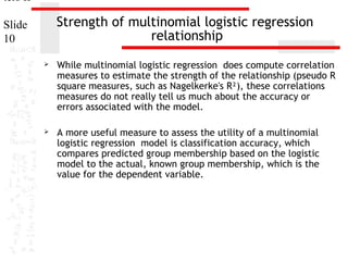
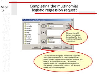
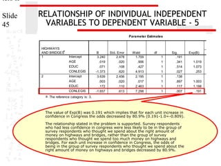
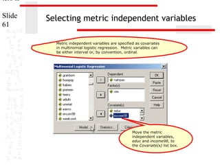
In the comparison of survey respondents who thought we spend
about the right amount of money on highways and bridges to
survey respondents who thought we spend too much money on
highways and bridges, the probability of the Wald statistic
(7.298) for the variable confidence in Congress [conlegis] was
0.007. Since the probability was less than or equal to the level
of significance of 0.05, the null hypothesis that the b coefficient
for confidence in Congress was equal to zero for this comparison
was rejected.
Exp(B)
95% Confiden
Exp
Lower Bound
1.019
1.073
.253
.980
.868
.075
1.003
1.188
.191
.963
.958
.057](https://image.slidesharecdn.com/multinomiallogisticregressionbasicrelationships-140123080904-phpapp02/85/Multinomial-logisticregression-basicrelationships-44-320.jpg)
![ters II
Slide
48
Answering the question in problem 1 - 1
11. In the dataset GSS2000, is the following statement true, false, or an incorrect application
of a statistic? Assume that there is no problem with missing data, outliers, or influential cases,
and that the validation analysis will confirm the generalizability of the results. Use a level of
significance of 0.05 for evaluating the statistical relationships.
The variables "age" [age], "highest year of school completed" [educ] and "confidence in
Congress" [conlegis] were useful predictors for distinguishing between groups based on
responses to "opinion about spending on highways and bridges" [natroad]. These predictors
differentiate survey respondents who thought we spend too little money on highways and
bridges from survey respondents who thought we spend too much money on highways and
bridges and survey respondents who thought we spend about the right amount of money on
highways and bridges from survey respondents who thought we spend too much money on
highways and bridges.
Among this set of predictors, confidence in Congress was helpful in distinguishing among the
groups defined by responses to opinion about spending on highways and bridges. Survey
We found a statistically significant be in
respondents who had less confidence in congress were less likely tooverallthe group of survey
relationship between highways and bridges, rather than the
respondents who thought we spend too little money onthe combination of
independent variables and the dependent
group of survey respondents who thought we spend too much money on highways and bridges.
variable.
For each unit increase in confidence in Congress, the odds of being in the group of survey
respondents who thought we spend too little money on highways and bridges decreased by
74.7%. Survey respondents who had less was no evidence of numerical less likelyin be in the
There confidence in congress were problems to
group of survey respondents who thought we spend about the right amount of money on
the solution.
highways and bridges, rather than the group of survey respondents who thought we spend too
much money on highways and bridges. For each unit increaseaccuracy surpassed
Moreover, the classification in confidence in Congress, the
odds of being in the group of survey respondents whochance accuracy criteria, the right amount
the proportional by thought we spend about
of money on highways and bridges supporting the 80.9%.of the model.
decreased by utility
1. True
2. True with caution
3. False](https://image.slidesharecdn.com/multinomiallogisticregressionbasicrelationships-140123080904-phpapp02/85/Multinomial-logisticregression-basicrelationships-48-320.jpg)
![ters II
Slide
49
Answering the question in problem 1 - 2
We verified that each statement about the [educ] and
The variables "age" [age], "highest year of school completed" relationship "confidence in
Congress" [conlegis]between an independent for distinguishingdependent groups based on
were useful predictors variable and the between
variable was correct in both direction of the relationship These predictors
responses to "opinion about spending on highways and bridges" [natroad].
differentiate surveyand the change in likelihoodwe spend too little money on highways and
respondents who thought associated with a one-unit
bridges from survey change of the who thought variable, for both of the
respondents independent we spend too much money on highways and
bridges and survey respondents who thought we stated in the problem. amount of money on
comparisons between groups spend about the right
highways and bridges from survey respondents who thought we spend too much money on
highways and bridges.
Among this set of predictors, confidence in Congress was helpful in distinguishing among the
groups defined by responses to opinion about spending on highways and bridges. Survey
respondents who had less confidence in congress were less likely to be in the group of survey
respondents who thought we spend too little money on highways and bridges, rather than the
group of survey respondents who thought we spend too much money on highways and bridges.
For each unit increase in confidence in Congress, the odds of being in the group of survey
respondents who thought we spend too little money on highways and bridges decreased by
74.7%. Survey respondents who had less confidence in congress were less likely to be in the
group of survey respondents who thought we spend about the right amount of money on
highways and bridges, rather than the group of survey respondents who thought we spend too
much money on highways and bridges. For each unit increase in confidence in Congress, the
odds of being in the group of survey respondents who thought we spend about the right amount
of money on highways and bridges decreased by 80.9%.
1.
2.
3.
4.
True
True with caution
False
Inappropriate application of a statistic
The answer to the question is true
with caution.
A caution is added because of the
inclusion of ordinal level variables.](https://image.slidesharecdn.com/multinomiallogisticregressionbasicrelationships-140123080904-phpapp02/85/Multinomial-logisticregression-basicrelationships-49-320.jpg)
![ters II
Slide
50
Problem 2
1. In the dataset GSS2000, is the following statement true, false, or an incorrect application of
a statistic? Assume that there is no problem with missing data, outliers, or influential cases,
and that the validation analysis will confirm the generalizability of the results. Use a level of
significance of 0.05 for evaluating the statistical relationships.
The variables "highest year of school completed" [educ], "sex" [sex] and "total family income"
[income98] were useful predictors for distinguishing between groups based on responses to
"opinion about spending on space exploration" [natspac]. These predictors differentiate survey
respondents who thought we spend too little money on space exploration from survey
respondents who thought we spend too much money on space exploration and survey
respondents who thought we spend about the right amount of money on space exploration from
survey respondents who thought we spend too much money on space exploration.
Among this set of predictors, total family income was helpful in distinguishing among the
groups defined by responses to opinion about spending on space exploration. Survey
respondents who had higher total family incomes were more likely to be in the group of survey
respondents who thought we spend about the right amount of money on space exploration,
rather than the group of survey respondents who thought we spend too much money on space
exploration. For each unit increase in total family income, the odds of being in the group of
survey respondents who thought we spend about the right amount of money on space
exploration increased by 6.0%.
1.
2.
3.
4.
True
True with caution
False
Inappropriate application of a statistic](https://image.slidesharecdn.com/multinomiallogisticregressionbasicrelationships-140123080904-phpapp02/85/Multinomial-logisticregression-basicrelationships-50-320.jpg)
![ters II
Slide
51
Dissecting problem 2 - 1
1. In the dataset GSS2000, is the following statement true, false, or an incorrect
application of a statistic? Assume that there is no problem with missing data, outliers, or
influential cases, and that the validation analysis will confirm the generalizability of the
results. Use a level of significance of 0.05 for evaluating the statistical relationships.
The variables "highest year of school completed" [educ], "sex" [sex] and "total family income"
[income98] were useful predictors for distinguishing between groups based on responses to
"opinion about spending on space exploration" [natspac]. we will predictors differentiate survey
For these problems, These
respondents who thought we spend too little money on is no problem
assume that there space exploration from survey
respondents who thought we spend too much money on outliers, or
with missing data, space exploration and survey
respondents who thought we spend about the right amount of money on space exploration from
influential cases, and that the
survey respondents who thought we spend too much moneyconfirm exploration.
on space
validation analysis will
the generalizability of the
Among this set of predictors, total family income was helpful in distinguishing among the
results
groups defined by responses to opinion about spending on space exploration. Survey
respondents who had higher total familythis problem, we are told to to be in the group of survey
In incomes were more likely
respondents who thought we spend about0.05 right amount of money on space exploration,
use the as alpha for the
rather than the group of survey respondents who logistic regression. too much money on space
multinomial thought we spend
exploration. For each unit increase in total family income, the odds of being in the group of
survey respondents who thought we spend about the right amount of money on space
exploration increased by 6.0%.
1.
2.
3.
4.
True
True with caution
False
Inappropriate application of a statistic](https://image.slidesharecdn.com/multinomiallogisticregressionbasicrelationships-140123080904-phpapp02/85/Multinomial-logisticregression-basicrelationships-51-320.jpg)
![ters II
Slide
52
Dissecting problem 2 - 2
The variables listed first in the problem
statement are the independent variables
1. In (IVs): "highest year of is the following statement true, false, or an incorrect application of
the dataset GSS2000, school completed"
a statistic? Assume [sex] there is nofamily
[educ], "sex" that and "total problem with missing data, outliers, or influential cases,
and that the validation analysis will confirm the generalizability of the results. Use a level of
income" [income98].
significance of 0.05 for evaluating the statistical relationships.
The variables "highest year of school completed" [educ], "sex" [sex] and "total family
income" [income98] were useful predictors for distinguishing between groups based on
responses to "opinion about spending on space exploration" [natspac]. These predictors
differentiate survey respondents who thought we spend too little money on space exploration
from survey respondents who thought we spend too much money on space exploration and
survey respondents who thought we spend about the right amount of money on space
exploration from survey respondents who thought we spend too much money on space
The variable
exploration. used to define
groups is the dependent
variable (DV): "opinion about
Among this on space
spending set of predictors, total family income was helpful in distinguishing among the
groups defined by responses to opinion about spending on space exploration. Survey
exploration" [natspac].
respondents who had higher total family incomes were more likely to be in the group of survey
respondents who thought we spend about the right amount of money on space exploration,
rather than the group of survey respondents who thought we spend too much money on space
SPSS only odds of direct in
exploration. For each unit increase in total family income, thesupports being or the group of
simultaneous entry of independent
survey respondents who thought we spend about the right amount of money on space
variables in multinomial logistic
exploration increased by 6.0%.
1. True
2. True with caution
3. False
regression, so we have no choice of
method for entering variables.](https://image.slidesharecdn.com/multinomiallogisticregressionbasicrelationships-140123080904-phpapp02/85/Multinomial-logisticregression-basicrelationships-52-320.jpg)
![ters II
Slide
53
Dissecting problem 2 - 3
SPSS multinomial logistic regression models the relationship
by comparing each of the groups defined by the dependent
variable to the group with the highest code value.
1. In the dataset GSS2000,to opinion about spending ontrue, false, or an incorrect application of
The responses is the following statement the space
a statistic? Assume that there is no problem with missing data, outliers, or influential cases,
program were:
and that the1= Too little, 2 = About right, and 3 = Too much.
validation analysis will confirm the generalizability of the results. Use a level of
significance of 0.05 for evaluating the statistical relationships.
The variables "highest year of school completed" [educ], "sex" [sex] and "total family income"
[income98] were useful predictors for distinguishing between groups based on responses to
"opinion about spending on space exploration" [natspac]. These predictors differentiate
survey respondents who thought we spend too little money on space exploration from
survey respondents who thought we spend too much money on space exploration and
survey respondents who thought we spend about the right amount of money on space
exploration from survey respondents who thought we spend too much money on space
exploration.
Among this set of predictors, total family income was helpful in distinguishing among the
The analysis will result about spending on
groups defined by responses to opinion in two comparisons:space exploration. Survey
respondents who • survey respondents who thought we spend likely to be in the group of survey
had higher total family incomes were more too little money
versus survey respondents who amount of money on space
respondents who thought we spend about the rightthought we spend too much exploration,
money on space exploration
rather than the group of survey respondents who thought we spend too much money on space
• survey increase in total family income, the odds the being in the group of
exploration. For each unit respondents who thought we spend about of right
amount of money versus survey respondents who money on
survey respondents who thought we spend about the right amount ofthought we space
exploration increased by 6.0%.
spend too much money on space exploration.
1. True](https://image.slidesharecdn.com/multinomiallogisticregressionbasicrelationships-140123080904-phpapp02/85/Multinomial-logisticregression-basicrelationships-53-320.jpg)
![ters II
Slide
54
Dissecting problem 2 - 4
Each problem includes a statement about the
The variables "highest year of school completed" [educ], "sex" [sex] and "total family income"
[income98]relationship between onefor distinguishing between groups based on responses to
were useful predictors independent variable and
the dependenton space exploration" [natspac]. These predictors differentiate survey
"opinion about spending variable. The answer to the
problem is based on the stated relationship,
respondents who thought we spend too little money on space exploration from survey
respondents who thought we spend too much money on space exploration and survey
ignoring the relationships between the other
respondents who thought we spend about the right variable. of money on space exploration from
independent variables and the dependent amount
survey respondents who thought we spend too much money on space exploration.
Among this set of predictors, total family income was helpful in distinguishing among the
groups defined by responses to opinion about spending on space exploration. Survey
respondents who had higher total family incomes were more likely to be in the group of
survey respondents who thought we spend about the right amount of money on space
exploration, rather than the group of survey respondents who thought we spend too much
money on space exploration. For each unit increase in total family income, the odds of
being in the group of survey respondents who thought we spend about the right amount of
money on space exploration increased by 6.0%.
1.
2.
3.
4.
True
True with caution
This problem identifies a difference for only one
of the two comparisons based on the three values
False
Inappropriate application of a of the dependent variable.
statistic
Other problems will specify both of the possible
comparisons.](https://image.slidesharecdn.com/multinomiallogisticregressionbasicrelationships-140123080904-phpapp02/85/Multinomial-logisticregression-basicrelationships-54-320.jpg)
![ters II
Slide
55
Dissecting problem 2 - 5
The variables "highest year of school completed" [educ], "sex" [sex] and "total family income"
[income98] were useful predictors for distinguishing between groups based on responses to
"opinion about spending on space exploration" [natspac]. These predictors differentiate survey
respondents who thought we spend too little money on space exploration from survey
respondents who thought we spend too much money on space exploration and survey
respondents who thought we spend about the right amount of money on space exploration from
survey respondents who thought we spend too much money on space exploration.
Among this set of predictors, total family income was helpful in distinguishing among the
groups defined by responses to opinion about spending on space exploration. Survey
respondents who had higher total family incomes were more likely to be in the group of survey
respondents who thought we spend about the right amount of money on space exploration,
rather than the group of survey respondents who thought we spend too much money on space
exploration. For each unit increase in total family income, the odds of being in the group of
survey respondents who thought we spend about the right amount of money on space
exploration increased by 6.0%.
1.
2.
3.
4.
True
In order for the multinomial logistic regression
question to be true, the overall relationship must
True with caution
be statistically significant, there must be no
False
evidence of numerical problems, the classification
Inappropriate application of a statistic
accuracy rate must be substantially better than
could be obtained by chance alone, and the
stated individual relationship must be statistically
significant and interpreted correctly.](https://image.slidesharecdn.com/multinomiallogisticregressionbasicrelationships-140123080904-phpapp02/85/Multinomial-logisticregression-basicrelationships-55-320.jpg)
![ters II
Slide
56
LEVEL OF MEASUREMENT - 1
1. In the dataset GSS2000, is the following statement true, false, or an incorrect application of
a statistic? Assume that there is no problem with missing data, outliers, or influential cases,
and that the validation analysis will confirm the generalizability of the results. Use a level of
significance of 0.05 for evaluating the statistical relationships.
The variables "highest year of school completed" [educ], "sex" [sex] and "total family income"
[income98] were useful predictors for distinguishing between groups based on responses to
"opinion about spending on space exploration" [natspac]. These predictors differentiate
survey respondents who thought we spend too little money on space exploration from
survey respondents who thought we spend too much money on space exploration and
survey respondents who thought we spend about the right amount of money on space
exploration from survey respondents who thought we spend too much money on space
exploration.
Among this set of predictors, total family income was helpful in distinguishing among the
Multinomial opinion about spending on space
groups defined by responses tologistic regression requires that the exploration. Survey
dependent variable be non-metric and the
respondents who had higher total family incomes were more likely to be in the group of survey
independent variables be metric or dichotomous.
respondents who thought we spend about the right amount of money on space exploration,
rather than the group of survey respondents who thought we spend too much money on space
"Opinion about spending on space exploration"
exploration. For each unit increase in total family income, the odds of being in the group of
[natspac] is ordinal, satisfying the non-metric
survey respondentslevel of measurement requirement for the
who thought we spend about the right amount of money on space
exploration increased by 6.0%.
dependent variable.
1.
2.
3.
4.
It contains three categories: survey respondents
True
who thought we spend too little money, about
True with cautionright amount of money, and too much
the
money on space exploration.
False
Inappropriate application of a statistic](https://image.slidesharecdn.com/multinomiallogisticregressionbasicrelationships-140123080904-phpapp02/85/Multinomial-logisticregression-basicrelationships-56-320.jpg)
![ters II
Slide
57
LEVEL OF MEASUREMENT - 2
"Highest year of school
"Sex" [sex] is dichotomous,
completed" [educ] is interval,
satisfying the metric or
satisfying the metric or
dichotomous level of measurement
1. In the dataset GSS2000, is the following statement true, false, or an incorrect application of
dichotomous level of
requirement for independent
measurement Assume that there is no problem with missing data, outliers, or influential cases,
a statistic? requirement for
variables.
independent variables.
and that the validation analysis will confirm the generalizability of the results. Use a level of
significance of 0.05 for evaluating the statistical relationships.
The variables "highest year of school completed" [educ], "sex" [sex] and "total family
income" [income98] were useful predictors for distinguishing between groups based on
responses to "opinion about spending on space exploration" [natspac]. These predictors
differentiate survey respondents who thought we spend too little money on space exploration
from survey respondents who thought we spend too much money on space exploration and
survey respondents who thought we spend about the right amount of money on space
exploration from survey family income" [income98] we spend too much money on space
"Total respondents who thought is ordinal,
exploration.
satisfying the metric or dichotomous level of
measurement requirement for independent
variables. If we follow the convention of treating
Among this set of ordinal level total family incomevariables, the in distinguishing among the
predictors, variables as metric was helpful level
groups defined byof measurement requirementspending on space exploration. Survey
responses to opinion about for the analysis is
respondents who had higher total family incomes were not agree to be in the group of survey
satisfied. Since some data analysts do more likely
with this convention, a note of caution should money on space exploration,
respondents who thought we spend about the right amount of be
included in our interpretation.
rather than the group of survey respondents who thought we spend about the right amount of
money on space exploration. For each unit increase in total family income, the odds of being in
the group of survey respondents who thought we spend about the right amount of money on
space exploration increased by 6.0%.
1. True
2. True with caution](https://image.slidesharecdn.com/multinomiallogisticregressionbasicrelationships-140123080904-phpapp02/85/Multinomial-logisticregression-basicrelationships-57-320.jpg)
![ters II
Slide
67
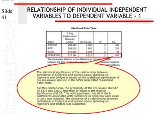
NUMERICAL PROBLEMS
Parameter Estimates
SPACE EXPLORATION
a
PROGRAM
1
2
Intercept
EDUC
INCOME98
[SEX=1]
[SEX=2]
Intercept
EDUC
INCOME98
[SEX=1]
[SEX=2]
B
Std. Error
-4.136
1.157
.101
.089
.097
.050
.672
.426
b
0
.
-2.487
.840
.108
.068
.058
.034
.501
.317
b
0
.
a. The reference category is: 3.
b. This parameter is set to zero because it is redundant.
Wald
12.779
1.276
3.701
2.488
.
8.774
2.521
2.932
2.492
.
df
95% Confidence
Exp(B)
Lower Bound
U
Sig.
Exp(B)
1
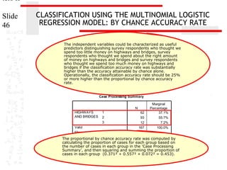
Multicollinearity .000
in the multinomial
logistic regression solution is
1
.259
1.106
detected by examining the
1
.054
1.102
standard errors for the b
1
.115
1.959
coefficients. A standard error
larger than 2.0 indicates numerical
0
.
.
problems, such .003
as multicollinearity
1
among the independent variables,
1
.112
1.114
zero cells for a dummy-coded
independent variable because all of
1
.087
1.060
the subjects have the same value
1
.114
1.650
for the variable, and 'complete
0
.
separation' whereby the two .
groups in the dependent event
variable can be perfectly separated
by scores on one of the
independent variables. Analyses
that indicate numerical problems
should not be interpreted.
None of the independent variables
in this analysis had a standard
error larger than 2.0.
.929
.998
.850
.
.975
.992
.886
.](https://image.slidesharecdn.com/multinomiallogisticregressionbasicrelationships-140123080904-phpapp02/85/Multinomial-logisticregression-basicrelationships-67-320.jpg)
![ters II
Slide
69
Answering the question in problem 2
1. In the dataset GSS2000, is the following statement true, false, or an incorrect application of
a statistic? Assume that there is no problem with missing data, outliers, or influential cases,
and that the validation analysis will confirm the generalizability of the results. Use a level of
significance of 0.05 for evaluating the statistical relationships.
The variables "highest year of school completed" [educ], "sex" [sex] and "total family income"
[income98] were useful predictors for distinguishing between groups based on responses to
"opinion about spending on space exploration" [natspac]. These predictors differentiate survey
respondents who thought we spend too little money on space exploration from survey
respondents who thought we spend too much money on space exploration and survey
respondents who thought we spend about the right amount of money on space exploration from
survey respondents who thought we spend too much money on space exploration.
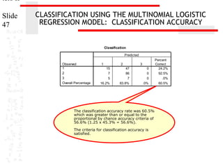
We found a statistically significant overall
relationship between the combination of
Among this set of predictors, totalindependent variables and the dependent
family income was helpful in distinguishing among the
groups defined by responses to opinion about spending on space exploration. Survey
variable.
respondents who had higher total family incomes were more likely to be in the group of survey
respondents who thought we spend about the right amount numerical problems in
There was no evidence of of money on space exploration,
rather than the group of survey respondents who thought we spend too much money on space
the solution.
exploration. For each unit increase in total family income, the odds of being in the group of
survey respondents who thought we spend about the right amount of money on space
However, the individual relationship between
exploration increased by 6.0%.
1.
2.
3.
4.
total family income and spending on space was
not statistically significant.
True
True with caution
The answer to the question is false.
False
Inappropriate application of a statistic](https://image.slidesharecdn.com/multinomiallogisticregressionbasicrelationships-140123080904-phpapp02/85/Multinomial-logisticregression-basicrelationships-69-320.jpg)
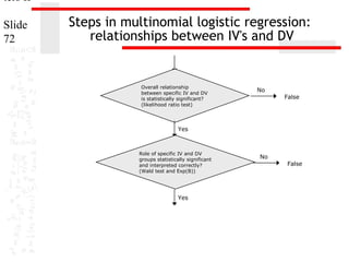
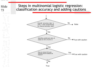

This document provides an overview of multinomial logistic regression. It discusses how multinomial logistic regression compares multiple groups through binary logistic regressions. It describes how to interpret the results, including evaluating the overall relationship between predictors and the dependent variable and relationships between individual predictors and the dependent variable. Requirements and assumptions of the analysis are explained, such as the dependent variable being non-metric and cases-to-variable ratios. Methods for evaluating model accuracy and usefulness are also outlined.