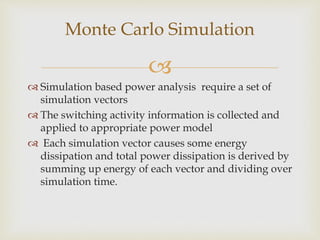
This document discusses Monte Carlo simulation techniques for power analysis of circuits. It explains that Monte Carlo simulation requires a large number of input vectors to accurately estimate power dissipation. The key points are: - Monte Carlo simulation collects switching activity from many input vectors to apply to a power model. - More input vectors lead to higher accuracy but diminishing returns. There is a point where additional vectors do not meaningfully improve accuracy. 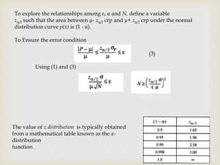- Statistical techniques can determine the optimal number of vectors needed to estimate power within a given error tolerance with a specific confidence level, such as 90%. This avoids wasting computation on unnecessary vectors.

1. By
Dr. Gargi Khanna
Department of Electronics & Communication
Engg.
NIT Hamirpur

2. 
Monte Carlo Simulation
 Simulation based power analysis require a set of
simulation vectors
 The switching activity information is collected and
applied to appropriate power model
 Each simulation vector causes some energy
dissipation and total power dissipation is derived by
summing up energy of each vector and dividing over
simulation time.

3. 
Monte Carlo Simulation
 How many input vectors are required for correct
estimation of Power dissipation??????
 How much extra accuracy can be achieved by
simulating million vectors vs thousand vectors.
Stopping Criteria for simulation

4. 
 Consider Basic sample period T in which a single
power dissipation value is observed.
E.g. T may be several vectors or several clock cycles.
The estimated power of circuit under
simulation is given by average value of the
samples
𝑃 =
𝑝1+𝑝2+𝑝3+⋯……..𝑝𝑛
𝑛
 classical mean estimation
Statistical Estimation of mean

5. 
 In statistics we draw N samples from a large
population and try to find mean of population.
 For small value of N, P is not truthful and
 for large N unnecessary computation will be
performed without gaining meaningful accuracy.
Statistical Estimation of mean
The
stopping
criteria
Determine
the sample
size N

6.  Let pi are random variables following unknown
probability density function. The distribution of pi depends
on the circuit, simulation vectors and sample intervals.
 Let µ and σ2 mean and variance of pi, Now the question is
how accurate is P in estimating µ with N samples?
 According to the well-known central limit theorem in
statistics, the sample mean P approaches the normal
distribution for large N regardless of the distribution of Pi'
 Assume that the samples Pi have normal distribution.
 Basic statistical theory states that the average of normally
distributed random variables also has normal distribution.
The mean of P is exactly µ and its variance is
𝜎𝜌
2=
𝜎2
𝑁
(1)

7. The normal distribution curve for P
To quantify the accuracy of the sample mean P, a maximum error tolerance
term is used, Given , find what is the probability that P is within the error
range of
the true mean
what is the probability for the condition??
0 ≤
𝑃−𝜇
𝜇
≤ 𝜀 (2)

8. The normal distribution curve for P
0 ≤
𝑃−𝜇
𝜇
≤ 𝜀 (2)
# If this probability is high, trust the estimate P; otherwise, increase the
sample size N to gain more confidence.
# The probability can be obtained by integrating the normal distribution
curve p(x).
# The probability is more conveniently expressed by a confidence
variable
The confidence level is defined as 100 (1 - )%. A confidence level of 100%
( = 0) means that P is absolutely within the error tolerance of e.
* Typically, the confidence level is set to more than 90% to be
meaningful.

9. To explore the relationships among , and N, define a variable
z /2 such that the area between µ- z /2 crp and µ+ z /2 crp under the nonnal
distribution curve p(x) is (1 - ).
To Ensure the error condition
(3)
Using (1) and (3)
The value of z distribution is typically obtained
from a mathematical table known as the z-
distribution
function.

10. # It is actually not very practical because actual mean and variance are
unknown quantities dependent on the circuit, simulation vectors and the
sample interval.
# For limited sample size find the sample average and sample variance
# The variables P and S2 are quantities that can be directly computed from
the observed N samples
# To get the confidence for measurement within desired level we would
change the z-distribution to the t-distribution. Thus to achieve a confidence
level of (1 - ) and an error tolerance of , the number of samples required is:

11. The procedure is summarized as follows:
1. Simulate to collect one sample Pi'
2. Evaluate sample mean P and variance S2 using Equation
3. Check if the inequality is satisfied; if so stop, else repeat from Step 1

12. 
1. Simulate to collect samples Pi‘
2. Evaluate sample mean P and variance S2
3. Check if the inequality is satisfied; if so stop, else
repeat from Step 1.
Monte carlo procedure

13. Thanks !!!
Stay Safe