1) Convolution represents a discrete-time (DT) or continuous-time (CT) linear time-invariant (LTI) system as the summation or integral of the input signal multiplied by the impulse response. 2) The impulse response completely characterizes an LTI system. 3) Convolution exploits the properties of time-invariance and linearity of LTI systems to represent the output of the system in terms of a convolution between the input and impulse response.

1. G H PATEL COLLEGE OF
ENGINEERING AND
TECHNOLOGY
SUB : SIGNAL &SYSTEM
BATCH : 1A09
BRANCH : ELECTRICAL
PREPERED BY:-
YASH KOTHADIA - 150110109019
ABHISHEK LALKIYA -150110109020
MAULIK VASOYA - 150110109060

2. CONVOLUTION

3.  Consider the DT system:
 If the input signal is and the system has no
energy at , the output
is called the impulse response of the system
[ ]y n[ ]x n
[ ]h n[ ]n
[ ] [ ]x n n
[ ] [ ]y n h n
System
System
0n 
DT Unit-Impulse Response

4.  Consider the DT system described by
 Its impulse response can be found to be
[ ] [ 1] [ ]y n ay n bx n  
( ) , 0,1,2,
[ ]
0, 1, 2, 3,
n
a b n
h n
n
 
 
   
EXAMPLE

5.  Let x[n] be an arbitrary input signal to a DT LTI system
 Suppose that for
 This signal can be represented as
0
[ ] [0] [ ] [1] [ 1] [2] [ 2]
[ ] [ ], 0,1,2,
i
x n x n x n x n
x i n i n
  



     
  
1, 2,n   [ ] 0x n 
PRESENTING SYSTEM IN TERM OF
SHIFTED AND SCALED IMPULS

6. 0
[ ] [ ] [ ], 0
i
y n x i h n i n


  
EXPLOTING TIME -
INVERIANCE AND LINEARITY

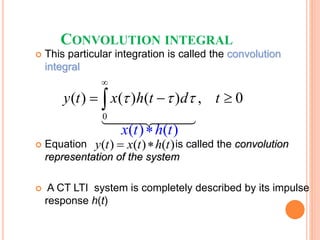
7.  This particular summation is called the convolution sum
 Equation is called the convolution
representation of the system.
 A DT LTI system is completely described by its impulse
response h[n].
0
[ ] [ ] [ ]
i
y n x i h n i


 
[ ] [ ]x n h n
[ ] [ ] [ ]y n x n h n 
CONVOLUTION SUM
(LINEAR CONVOLUTION)

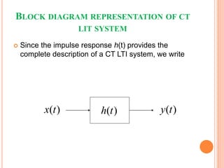
8.  Since the impulse response h[n] provides the
complete description of a DT LTI system, we write
[ ]y n[ ]x n [ ]h n
BLOCK DIAGRAM
REPRESENTATION OF DT LTI
SYSTEM

9.  Suppose that we have two signals x[n] and v[n] that
are not zero for negative times .
 Then, their convolution is expressed by the two-
sided series
[ ] [ ] [ ]
i
y n x i v n i


 
THE CONVOLUTION SUM FOR
NONCAUSAL SIGNALS

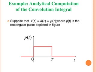
10.  Suppose that both x[n] and v[n] are equal to the
rectangular pulse p[n] (causal signal) represent
below
EXAMPLE: CONVOLUTION OF TWO
RECTANGULAR PULSES

11.  The signal is equal to the pulse p[i] folded about
the vertical axis
[ ]v i
THE FOLDED PULS

12. SHIFTING V[N- I] OVER X[I]

13. PLOT OF X[N]*V[N]

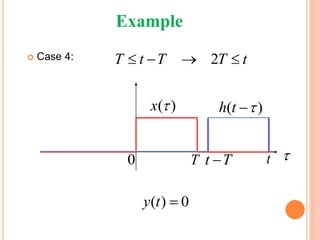
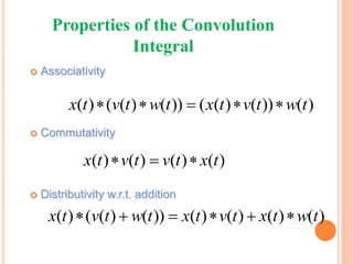
14.  Associatively
 Commutatively
 Distributive w.r.t. addition
[ ] ( [ ] [ ]) ( [ ] [ ]) [ ]x n v n w n x n v n w n    
[ ] [ ] [ ] [ ]x n v n v n x n  
[ ] ( [ ] [ ]) [ ] [ ] [ ] [ ]x n v n w n x n v n x n w n     
PROPERTIES OF CONVOLUTION SUM

15. CONVOLUTION INTEGRAL
 This particular integration is called the convolution
integral
 Equation is called the convolution
representation of the system
 A CT LTI system is completely described by its impulse
response h(t)
( ) ( )x t h t
( ) ( ) ( )y t x t h t 
0
( ) ( ) ( ) , 0y t x h t d t  

  

16.  Since the impulse response h(t) provides the
complete description of a CT LTI system, we write
( )y t( )x t ( )h t
BLOCK DIAGRAM REPRESENTATION OF CT
LIT SYSTEM

17.  Suppose that where p(t) is the
rectangular pulse depicted in figure
( ) ( ) ( ),x t h t p t 
( )p t
tT0
Example: Analytical Computation
of the Convolution Integral

18.  In order to compute the convolution integral
we have to consider four cases:
0
( ) ( ) ( ) , 0y t x h t d t  

  
Example

19.  Case 1: 0t 
( )x 
T0
( )h t 
t T t
( ) 0y t 
Example

20.  Case 2: 0 t T 
( )x 
T0
( )h t 
t T t
0
( )
t
y t d t 
Example

21.  Case 3:
( )x 
T0
( )h t 
t T t
( ) ( ) 2
T
t T
y t d T t T T t

     
0 2t T T T t T     
Example

22.  Case 4:
( ) 0y t 
( )x 
T0
( )h t 
t T t
2T t T T t   
Example

23.  Associativity
 Commutativity
 Distributivity w.r.t. addition
( ) ( ( ) ( )) ( ( ) ( )) ( )x t v t w t x t v t w t    
( ) ( ) ( ) ( )x t v t v t x t  
( ) ( ( ) ( )) ( ) ( ) ( ) ( )x t v t w t x t v t x t w t     
Properties of the Convolution
Integral