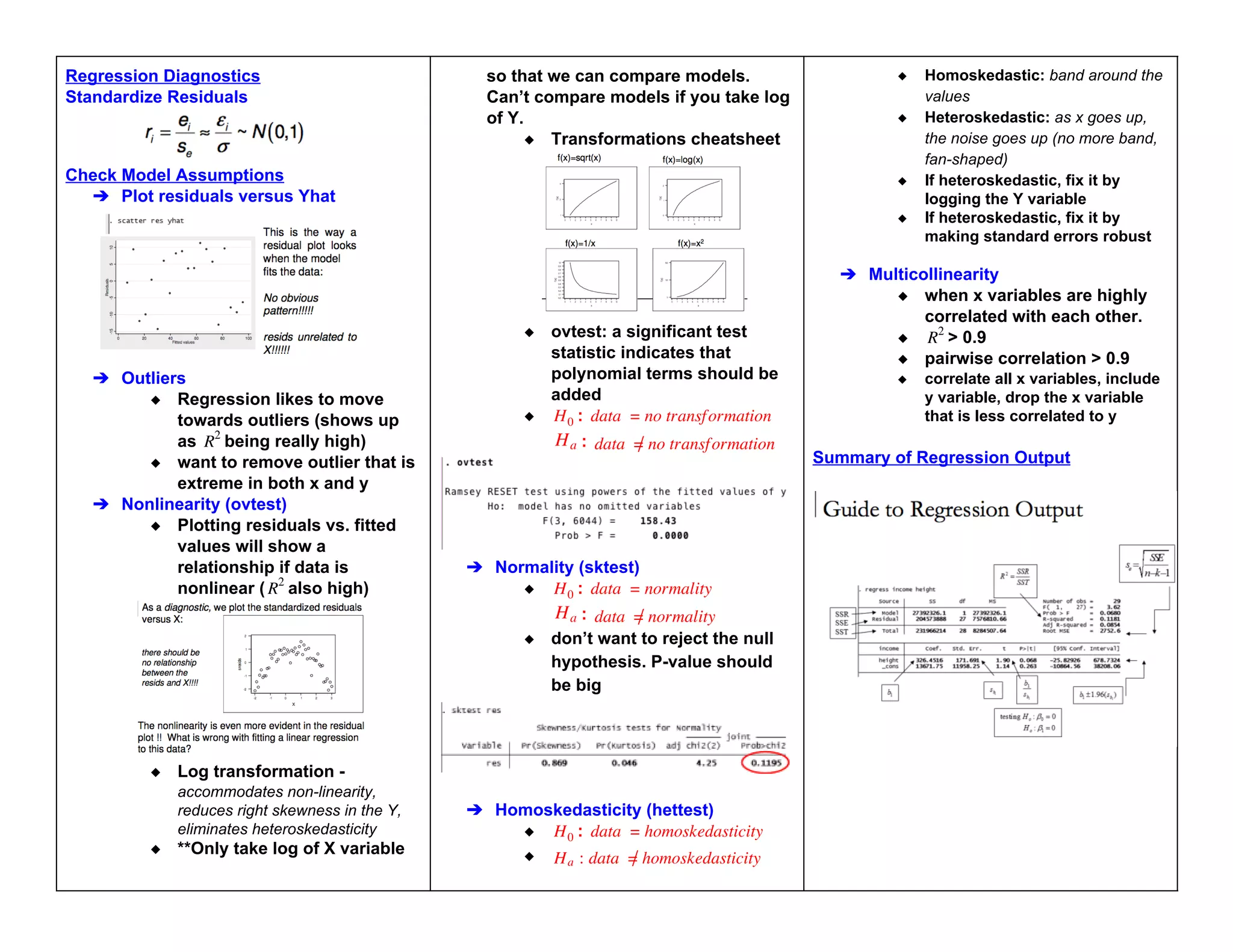
This document provides an overview of key concepts in statistics and probability, including: - Population and sample definitions and sampling techniques - Descriptive statistics such as mean, median, variance, and standard deviation - Probability rules and concepts like independent and mutually exclusive events - Common probability distributions like the binomial, normal, and uniform distributions - 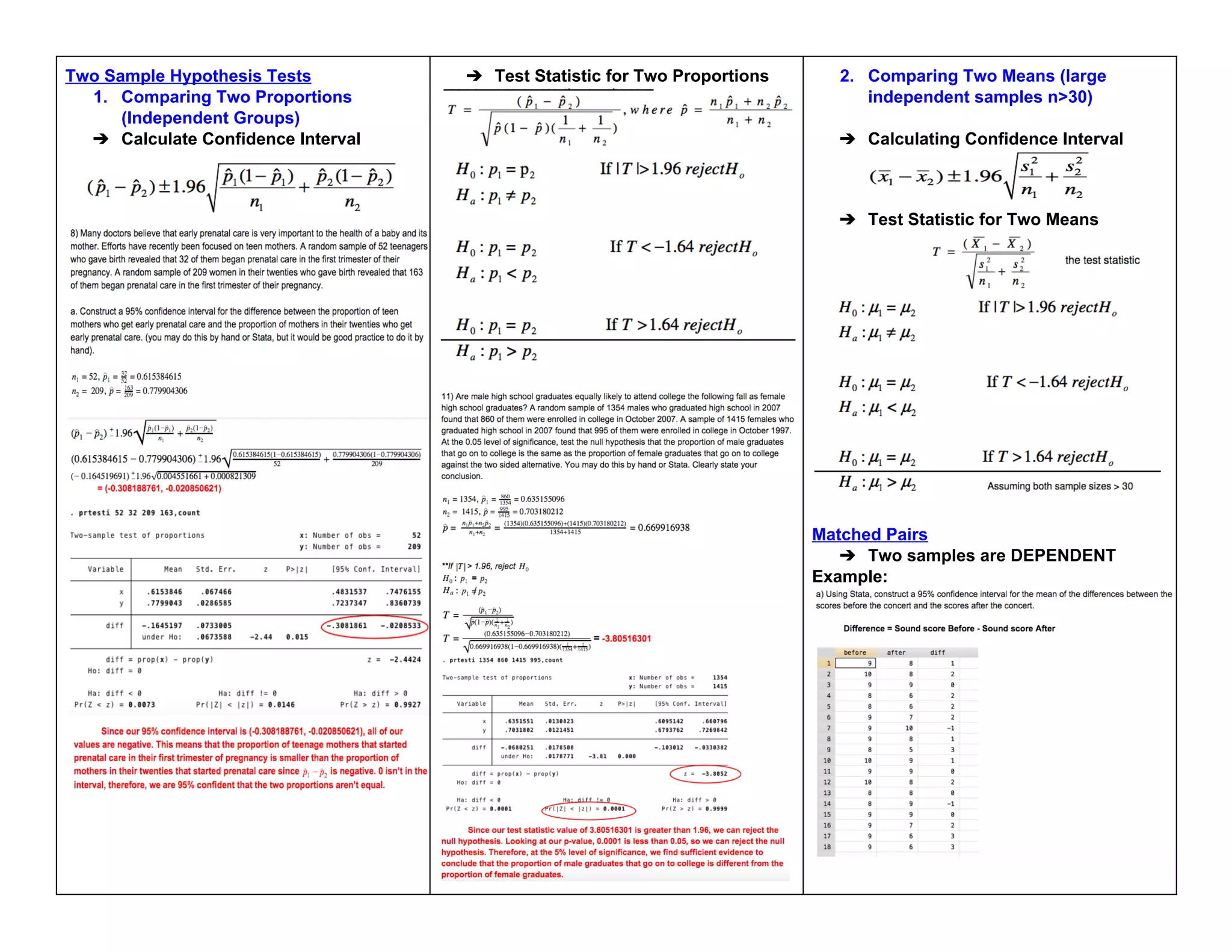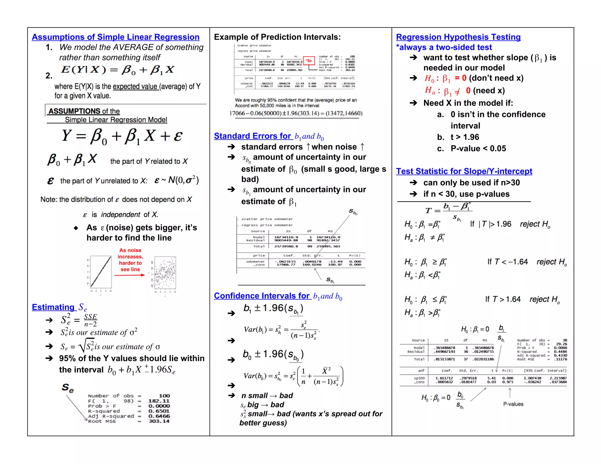Hypothesis testing methods using confidence intervals and p-values - 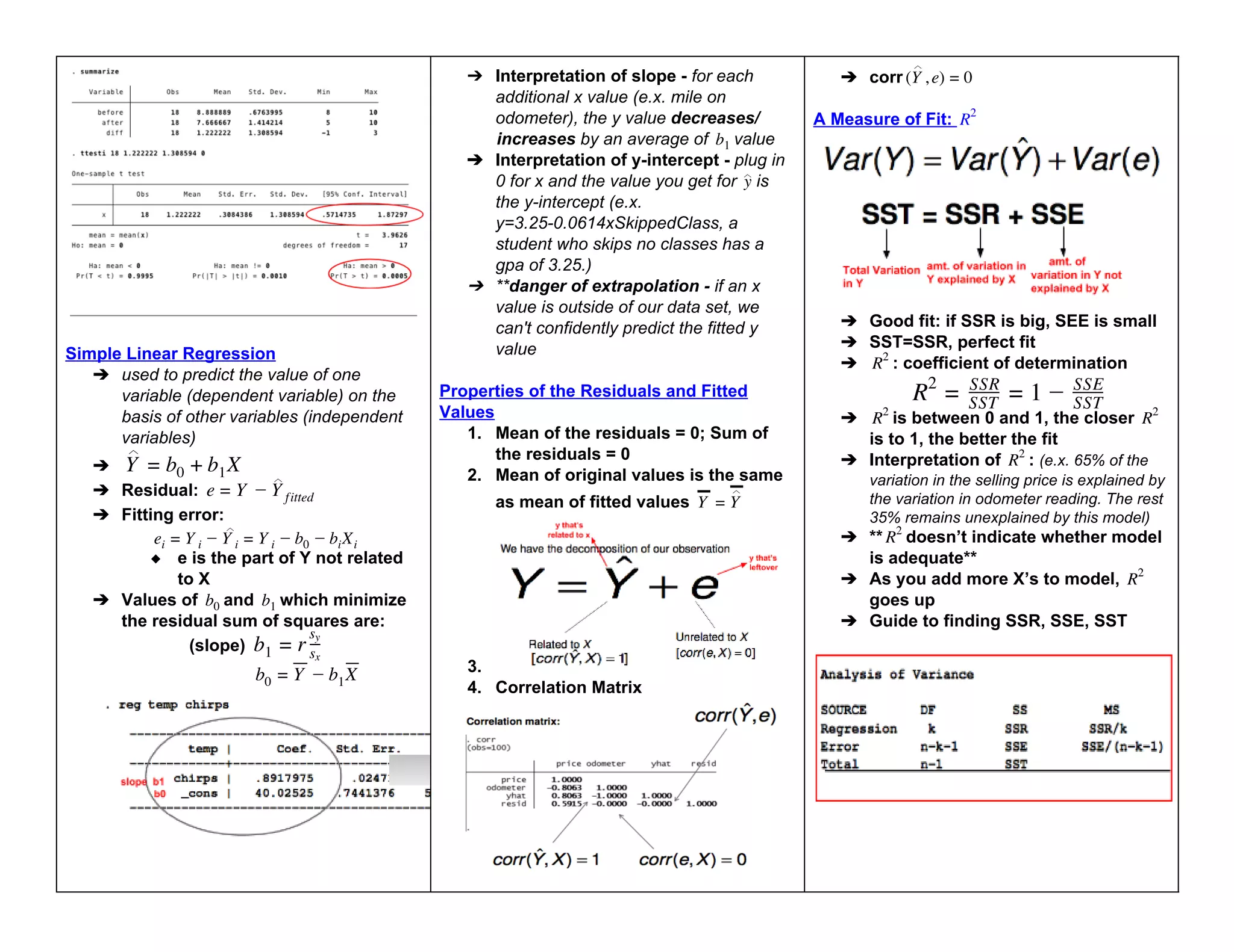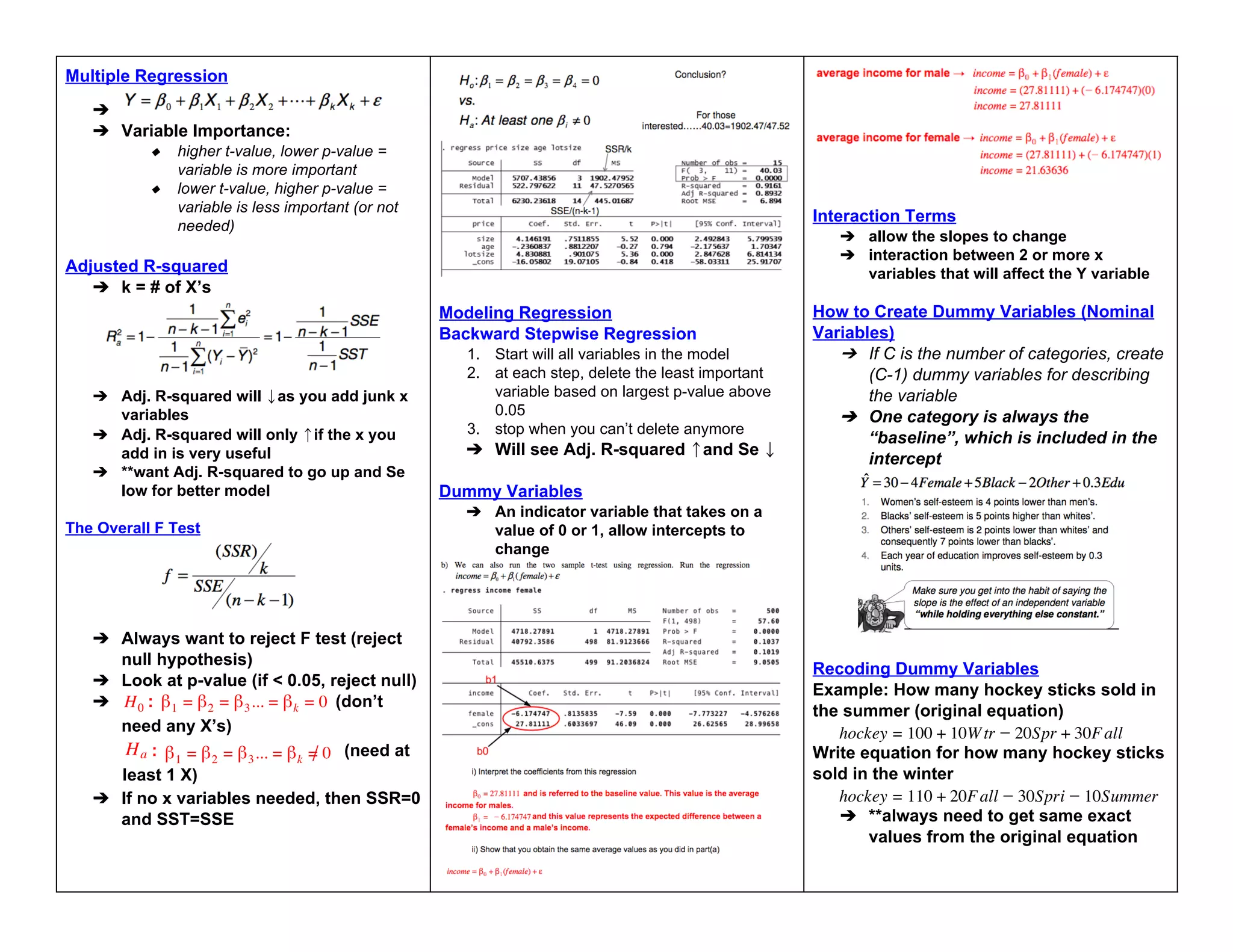Simple linear regression to model relationships between variables The document covers a wide range of foundational statistical topics in a detailed yet accessible manner.

1. Population ­ entire collection of objects or
individuals about which information is desired.
➔ easier to take a sample
◆ Sample ­ part of the population
that is selected for analysis
◆ Watch out for:
● Limited sample size that
might not be
representative of
population
◆ Simple Random Sampling­
Every possible sample of a certain
size has the same chance of being
selected
Observational Study ­ there can always be
lurking variables affecting results
➔ i.e, strong positive association between
shoe size and intelligence for boys
➔ **should never show causation
Experimental Study­ lurking variables can be
controlled; can give good evidence for causation
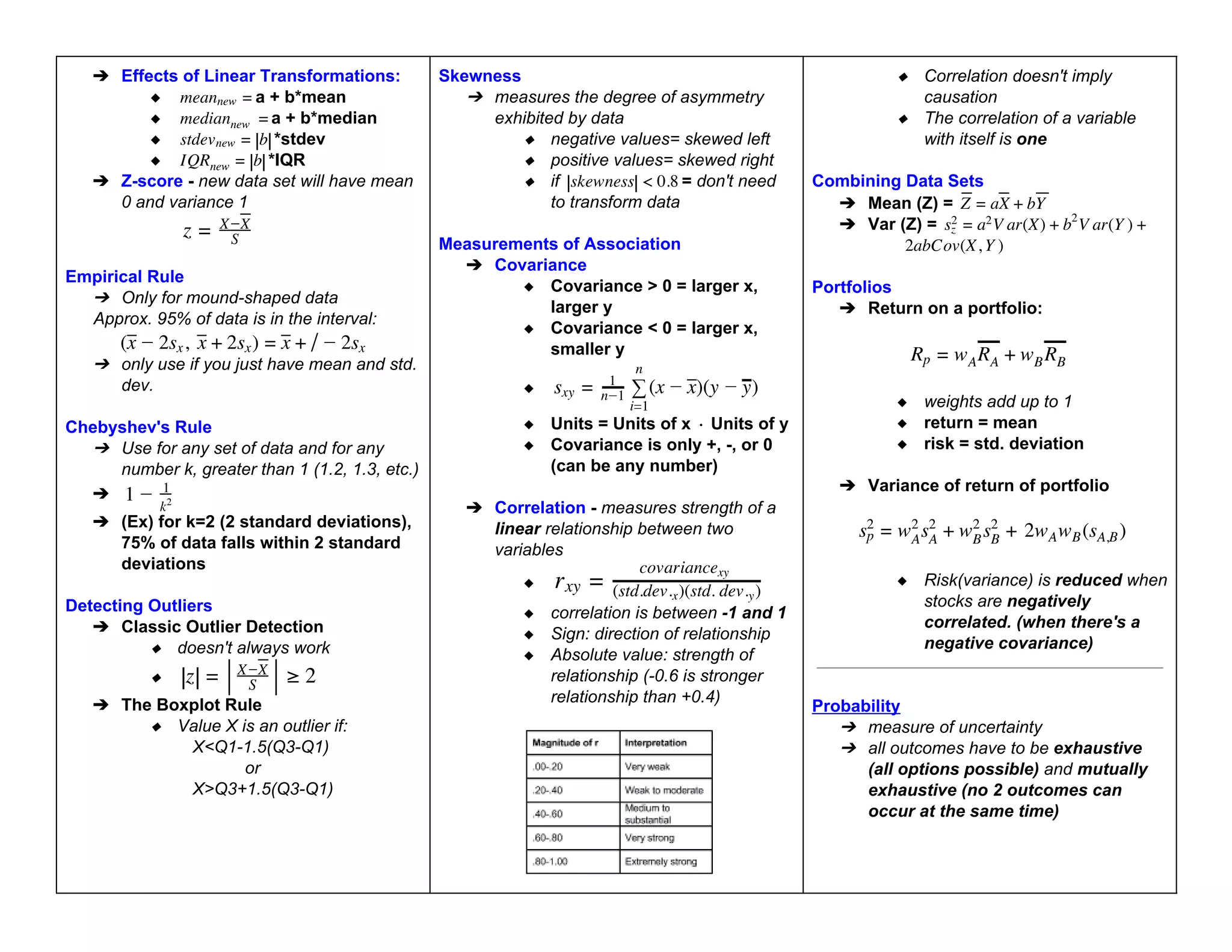
Descriptive Statistics Part I
➔ Summary Measures
➔ Mean ­ arithmetic average of data
values
◆ **Highly susceptible to
extreme values (outliers).
Goes towards extreme values
◆ Mean could never be larger or
smaller than max/min value but
could be the max/min value
➔ Median ­ in an ordered array, the
median is the middle number
◆ **Not affected by extreme
values
➔ Quartiles ­ split the ranked data into 4
equal groups
◆ Box and Whisker Plot
➔ Range = Xmaximum Xminimum
◆ Disadvantages: Ignores the
way in which data are
distributed; sensitive to outliers
➔ Interquartile Range (IQR) = 3rd
quartile ­ 1st quartile
◆ Not used that much
◆ Not affected by outliers
➔ Variance ­ the average distance
squared
sx
2 = n 1
(x x)
∑
n
i=1
i
2
◆ gets rid of the negative
sx
2
values
◆ units are squared
➔ Standard Deviation ­ shows variation
about the mean
s =
√ n 1
(x x)
∑
n
i=1
i
2
◆ highly affected by outliers
◆ has same units as original
data
◆ finance = horrible measure of
risk (trampoline example)
Descriptive Statistics Part II
Linear Transformations
➔ Linear transformations change the
center and spread of data
➔ ar(a X) V ar(X)
V + b = b2
➔ Average(a+bX) = a+b[Average(X)]
STAT 100 Final Cheat Sheets - Harvard University

2. ➔ Effects of Linear Transformations:
◆ a + b*mean
meannew =
◆ a + b*median
mediannew =
◆ *stdev
stdevnew = b
| |
◆ *IQR
IQRnew = b
| |
➔ Z­score ­ new data set will have mean
0 and variance 1
z = S
X X
Empirical Rule
➔ Only for mound­shaped data
Approx. 95% of data is in the interval:
x s , x s ) s
( 2 x + 2 x = x + / 2 x
➔ only use if you just have mean and std.
dev.
Chebyshev's Rule
➔ Use for any set of data and for any
number k, greater than 1 (1.2, 1.3, etc.)
➔ 1 1
k2
➔ (Ex) for k=2 (2 standard deviations),
75% of data falls within 2 standard
deviations
Detecting Outliers
➔ Classic Outlier Detection
◆ doesn't always work
◆ z
| | = |
| S
X X |
| ≥ 2
➔ The Boxplot Rule
◆ Value X is an outlier if:
X<Q1­1.5(Q3­Q1)
or
X>Q3+1.5(Q3­Q1)
Skewness
➔ measures the degree of asymmetry
exhibited by data
◆ negative values= skewed left
◆ positive values= skewed right
◆ if = don't need
.8
skewness
| | < 0
to transform data
Measurements of Association
➔ Covariance
◆ Covariance > 0 = larger x,
larger y
◆ Covariance < 0 = larger x,
smaller y
◆ s (x )(y )
xy = 1
n 1 ∑
n
i=1
x y
◆ Units = Units of x Units of y
◆ Covariance is only +, ­, or 0
(can be any number)
➔ Correlation ­ measures strength of a
linear relationship between two
variables
◆ rxy =
covariancexy
(std.dev. )(std. dev. )
x y
◆ correlation is between ­1 and 1
◆ Sign: direction of relationship
◆ Absolute value: strength of
relationship (­0.6 is stronger
relationship than +0.4)
◆ Correlation doesn't imply
causation
◆ The correlation of a variable
with itself is one
Combining Data Sets
➔ Mean (Z) = X Y
Z = a + b
➔ Var (Z) = V ar(X) V ar(Y )
sz
2 = a2 + b2
+
abCov(X, )
2 Y
Portfolios
➔ Return on a portfolio:
R R
Rp = wA A + wB B
◆ weights add up to 1
◆ return = mean
◆ risk = std. deviation
➔ Variance of return of portfolio
s s
s2
p = w2
A
2
A + w2
B
2
B + w w (s )
2 A B A,B
◆ Risk(variance) is reduced when
stocks are negatively
correlated. (when there's a
negative covariance)
Probability
➔ measure of uncertainty
➔ all outcomes have to be exhaustive
(all options possible) and mutually
exhaustive (no 2 outcomes can
occur at the same time)

3. Probability Rules
1. Probabilities range from
rob(A)
0 ≤ P ≤ 1
2. The probabilities of all outcomes must
add up to 1
3. The complement rule = A happens
or A doesn't happen
(A) (A)
P = 1 P
(A) (A)
P + P = 1
4. Addition Rule:
(A or B) (A) (B) (A and B)
P = P + P P
Contingency/Joint Table
➔ To go from contingency to joint table,
divide by total # of counts
➔ everything inside table adds up to 1
Conditional Probability
➔ (A|B)
P
➔ (A|B)
P = P(B)
P(A and B)
➔ Given event B has happened, what is
the probability event A will happen?
➔ Look out for: "given", "if"
Independence
➔ Independent if:
or
(A|B) (A)
P = P (B|A) (B)
P = P
➔ If probabilities change, then A and B
are dependent
➔ **hard to prove independence, need
to check every value
Multiplication Rules
➔ If A and B are INDEPENDENT:
(A and B) (A) (B)
P = P P
➔ Another way to find joint probability:
(A and B) (A|B) (B)
P = P P
(A and B) (B|A) (A)
P = P P
2 x 2 Table
Decision Analysis
➔ Maximax solution = optimistic
approach. Always think the best is
going to happen
➔ Maximin solution = pessimistic
approach.
➔ Expected Value Solution =
MV (P ) (P )... (P )
E = X1 1 + X2 2 + Xn n
Decision Tree Analysis
➔ square = your choice
➔ circle = uncertain events
Discrete Random Variables
➔ (x) (X )
PX = P = x
Expectation
➔ = E(x) =
μx P(X )
∑xi = xi
➔ Example: 2)(0.1) 3)(0.5) .7
( + ( = 1
Variance
➔ (x )
σ2
= E 2
μx
2
➔ Example:
2) (0.1) 3) (0.5) 1.7) .01
( 2
+ ( 2
( 2
= 2
Rules for Expectation and Variance
➔ (s) a bμ
μs = E = + x
➔ Var(s)= b2
σ2
Jointly Distributed Discrete Random
Variables
➔ Independent if:
(X and Y ) (x) (y)
Px,y = x = y = Px Py

4. ➔ Combining Random Variables
◆ If X and Y are independent:
(X ) (X) (Y )
E + Y = E + E
ar(X ) ar(X) ar(Y )
V + Y = V + V
◆ If X and Y are dependent:
(X ) (X) (Y )
E + Y = E + E
ar(X ) ar(X) ar(Y ) Cov(X, )
V + Y = V + V + 2 Y
➔ Covariance:
ov(X, ) (XY ) (X)E(Y )
C Y = E E
➔ If X and Y are independent, Cov(X,Y)
= 0
Binomial Distribution
➔ doing something n times
➔ only 2 outcomes: success or failure
➔ trials are independent of each other
➔ probability remains constant
1.) All Failures
(all failures) 1 )
P = ( p n
2.) All Successes
(all successes)
P = pn
3.) At least one success
(at least 1 success) 1 )
P = 1 ( p n
4.) At least one failure
P(at least 1 failure) = 1 pn
5.) Binomial Distribution Formula for
x=exact value
6.) Mean (Expectation)
(x) p
μ = E = n
7.) Variance and Standard Dev.
pq
σ2
= n
σ = √npq
q = 1 p
Binomial Example
Continuous Probability Distributions
➔ the probability that a continuous
random variable X will assume any
particular value is 0
➔ Density Curves
◆ Area under the curve is the
probability that any range of
values will occur.
◆ Total area = 1
Uniform Distribution
◆ nif (a, )
X ~ U b
Uniform Example
(Example cont'd next page)

5. ➔ Mean for uniform distribution:
(X)
E = 2
(a+b)
➔ Variance for unif. distribution:
ar(X)
V = 12
(b a)2
Normal Distribution
➔ governed by 2 parameters:
(the mean) and (the standard
μ σ
deviation)
➔ (μ, )
X ~ N σ2
Standardize Normal Distribution:
Z = σ
X μ
➔ Z­score is the number of standard
deviations the related X is from its
mean
➔ **Z< some value, will just be the
probability found on table
➔ **Z> some value, will be
(1­probability) found on table
Normal Distribution Example
Sums of Normals
Sums of Normals Example:
➔ Cov(X,Y) = 0 b/c they're independent
Central Limit Theorem
➔ as n increases,
➔ should get closer to (population
x μ
mean)
➔ mean( )
x = μ
➔ variance x) n
( = σ2
/
➔ (μ, )
X ~ N n
σ2
◆ if population is normally distributed,
n can be any value
◆ any population, n needs to be 0
≥ 3
➔ Z =
X μ
σ/√n
Confidence Intervals = tells us how good our
estimate is
**Want high confidence, narrow interval
**As confidence increases , interval also
increases
A. One Sample Proportion
➔ p
︿
= x
n = sample size
number of successes in sample
➔
➔ We are thus 95% confident that the true
population proportion is in the interval…
➔ We are assuming that n is large, n >5 and
p
︿
our sample size is less than 10% of the
population size.

6. Standard Error and Margin of Error
Example of Sample Proportion Problem
Determining Sample Size
n = e2
(1.96) p(1 p)
2︿ ︿
➔ If given a confidence interval, is
p
︿
the middle number of the interval
➔ No confidence interval; use worst
case scenario
◆ =0.5
p
︿
B. One Sample Mean
For samples n > 30
Confidence Interval:
➔ If n > 30, we can substitute s for
so that we get:
σ
For samples n < 30
T Distribution used when:
➔ is not known, n < 30, and data is
σ
normally distributed
*Stata always uses the t­distribution when
computing confidence intervals
Hypothesis Testing
➔ Null Hypothesis:
➔ , a statement of no change and is
H0
assumed true until evidence indicates
otherwise.
➔ Alternative Hypothesis: is a
Ha
statement that we are trying to find
evidence to support.
➔ Type I error: reject the null hypothesis
when the null hypothesis is true.
(considered the worst error)
➔ Type II error: do not reject the null
hypothesis when the alternative
hypothesis is true.
Example of Type I and Type II errors
Methods of Hypothesis Testing
1. Confidence Intervals **
2. Test statistic
3. P­values **
➔ C.I and P­values always safe to do
because don’t need to worry about
size of n (can be bigger or smaller
than 30)

7. One Sample Hypothesis Tests
1. Confidence Interval (can be
used only for two­sided tests)
2. Test Statistic Approach
(Population Mean) 3. Test Statistic Approach (Population
Proportion)
4. P­Values
➔ a number between 0 and 1
➔ the larger the p­value, the more
consistent the data is with the null
➔ the smaller the p­value, the more
consistent the data is with the
alternative
➔ **If P is low (less than 0.05),
must go ­ reject the null
H0
hypothesis

8. Two Sample Hypothesis Tests
1. Comparing Two Proportions
(Independent Groups)
➔ Calculate Confidence Interval
➔ Test Statistic for Two Proportions 2. Comparing Two Means (large
independent samples n>30)
➔ Calculating Confidence Interval
➔ Test Statistic for Two Means
Matched Pairs
➔ Two samples are DEPENDENT
Example:

9. Simple Linear Regression
➔ used to predict the value of one
variable (dependent variable) on the
basis of other variables (independent
variables)
➔ X
Y
︿
= b0 + b1
➔ Residual: e = Y Y
︿
fitted
➔ Fitting error:
X
ei = Y i Y i
︿
= Y i b0 bi i
◆ e is the part of Y not related
to X
➔ Values of and which minimize
b0 b1
the residual sum of squares are:
(slope) b1 = rsx
sy
X
b0 = Y b1
➔ Interpretation of slope ­ for each
additional x value (e.x. mile on
odometer), the y value decreases/
increases by an average of value
b1
➔ Interpretation of y­intercept ­ plug in
0 for x and the value you get for is
y
︿
the y­intercept (e.x.
y=3.25­0.0614xSkippedClass, a
student who skips no classes has a
gpa of 3.25.)
➔ **danger of extrapolation ­ if an x
value is outside of our data set, we
can't confidently predict the fitted y
value
Properties of the Residuals and Fitted
Values
1. Mean of the residuals = 0; Sum of
the residuals = 0
2. Mean of original values is the same
as mean of fitted values Y = Y
︿
3.
4. Correlation Matrix
➔ corr Y , )
(
︿
e = 0
A Measure of Fit: R2
➔ Good fit: if SSR is big, SEE is small
➔ SST=SSR, perfect fit
➔ : coefficient of determination
R2
R2
= SSR
SST = 1 SST
SSE
➔ is between 0 and 1, the closer
R2
R2
is to 1, the better the fit
➔ Interpretation of : (e.x. 65% of the
R2
variation in the selling price is explained by
the variation in odometer reading. The rest
35% remains unexplained by this model)
➔ ** doesn’t indicate whether model
R2
is adequate**
➔ As you add more X’s to model, R2
goes up
➔ Guide to finding SSR, SSE, SST

10. Assumptions of Simple Linear Regression
1. We model the AVERAGE of something
rather than something itself
2.
◆ As (noise) gets bigger, it’s
ε
harder to find the line
Estimating Se
➔ S2
e = n 2
SSE
➔ is our estimate of σ
Se
2 2
➔ is our estimate of σ
Se = √Se
2
➔ 95% of the Y values should lie within
the interval X 1.96S
b0 + b1
+
e
Example of Prediction Intervals:
Standard Errors for and b
b1 0
➔ standard errors when noise
➔ amount of uncertainty in our
sb0
estimate of (small s good, large s
β0
bad)
➔ amount of uncertainty in our
sb1
estimate of β1
Confidence Intervals for and b
b1 0
➔
➔
➔
➔
➔ n small → bad
big → bad
se
small→ bad (wants x’s spread out for
s2
x
better guess)
Regression Hypothesis Testing
*always a two­sided test
➔ want to test whether slope ( ) is
β1
needed in our model
➔ : = 0 (don’t need x)
H0 β1
: 0 (need x)
Ha =
β1 /
➔ Need X in the model if:
a. 0 isn’t in the confidence
interval
b. t > 1.96
c. P­value < 0.05
Test Statistic for Slope/Y­intercept
➔ can only be used if n>30
➔ if n < 30, use p­values

11. Multiple Regression
➔
➔ Variable Importance:
◆ higher t­value, lower p­value =
variable is more important
◆ lower t­value, higher p­value =
variable is less important (or not
needed)
Adjusted R­squared
➔ k = # of X’s
➔ Adj. R­squared will as you add junk x
variables
➔ Adj. R­squared will only if the x you
add in is very useful
➔ **want Adj. R­squared to go up and Se
low for better model
The Overall F Test
➔ Always want to reject F test (reject
null hypothesis)
➔ Look at p­value (if < 0.05, reject null)
➔ : (don’t
H0 ...
β1 = β2 = β3 = βk = 0
need any X’s)
: (need at
Ha ... =
β1 = β2 = β3 = βk / 0
least 1 X)
➔ If no x variables needed, then SSR=0
and SST=SSE
Modeling Regression
Backward Stepwise Regression
1. Start will all variables in the model
2. at each step, delete the least important
variable based on largest p­value above
0.05
3. stop when you can’t delete anymore
➔ Will see Adj. R­squared and Se
Dummy Variables
➔ An indicator variable that takes on a
value of 0 or 1, allow intercepts to
change
Interaction Terms
➔ allow the slopes to change
➔ interaction between 2 or more x
variables that will affect the Y variable
How to Create Dummy Variables (Nominal
Variables)
➔ If C is the number of categories, create
(C­1) dummy variables for describing
the variable
➔ One category is always the
“baseline”, which is included in the
intercept
Recoding Dummy Variables
Example: How many hockey sticks sold in
the summer (original equation)
ockey 00 0Wtr 0Spr 0Fall
h = 1 + 1 2 + 3
Write equation for how many hockey sticks
sold in the winter
ockey 10 0Fall 0Spri 0Summer
h = 1 + 2 3 1
➔ **always need to get same exact
values from the original equation

12. Regression Diagnostics
Standardize Residuals
Check Model Assumptions
➔ Plot residuals versus Yhat
➔ Outliers
◆ Regression likes to move
towards outliers (shows up
as being really high)
R2
◆ want to remove outlier that is
extreme in both x and y
➔ Nonlinearity (ovtest)
◆ Plotting residuals vs. fitted
values will show a
relationship if data is
nonlinear ( also high)
R2
◆ Log transformation ­
accommodates non­linearity,
reduces right skewness in the Y,
eliminates heteroskedasticity
◆ **Only take log of X variable
so that we can compare models.
Can’t compare models if you take log
of Y.
◆ Transformations cheatsheet
◆ ovtest: a significant test
statistic indicates that
polynomial terms should be
added
◆ :
H0 ata o transformation
d = n
:
Ha ata = o transformation
d / n
➔ Normality (sktest)
◆ :
H0 ata ormality
d = n
:
Ha ata = ormality
d / n
◆ don’t want to reject the null
hypothesis. P­value should
be big
➔ Homoskedasticity (hettest)
◆ :
H0 ata omoskedasticity
d = h
◆ ata = omoskedasticity
Ha : d / h
◆ Homoskedastic: band around the
values
◆ Heteroskedastic: as x goes up,
the noise goes up (no more band,
fan­shaped)
◆ If heteroskedastic, fix it by
logging the Y variable
◆ If heteroskedastic, fix it by
making standard errors robust
➔ Multicollinearity
◆ when x variables are highly
correlated with each other.
◆ > 0.9
R2
◆ pairwise correlation > 0.9
◆ correlate all x variables, include
y variable, drop the x variable
that is less correlated to y
Summary of Regression Output
Source: http://people.fas.harvard.edu/~mparzen/stat100/Stat%20100%20Final%20Cheat%20Sheets%20Docs%20(2).pdf