Text similarity measures are used to quantify the similarity between text strings and documents. Common text similarity measures include Levenshtein distance for word similarity and cosine similarity for document similarity. To apply cosine similarity, documents first need to be represented in a document-term matrix using techniques like count vectorization or TF-IDF. TF-IDF is often preferred as it assigns higher importance to rare terms compared to common terms.

1. Text Similarity Measures

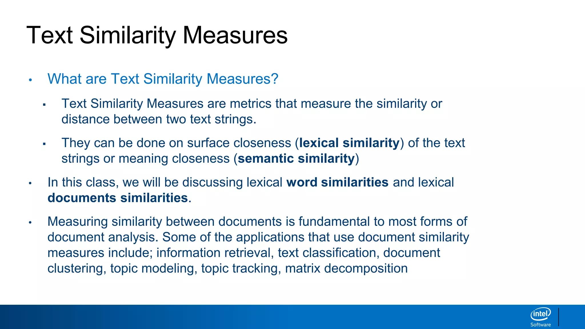
2. Text Similarity Measures
• What are Text Similarity Measures?
▪ Text Similarity Measures are metrics that measure the similarity or
distance between two text strings.
▪ They can be done on surface closeness (lexical similarity) of the text
strings or meaning closeness (semantic similarity)
• In this class, we will be discussing lexical word similarities and lexical
documents similarities.
• Measuring similarity between documents is fundamental to most forms of
document analysis. Some of the applications that use document similarity
measures include; information retrieval, text classification, document
clustering, topic modeling, topic tracking, matrix decomposition

3. Text Similarity Measures
• Word Similarity
▪ Levenshtein distance
• Document Similarity
▪ Count vectorizer and the document-term matrix
▪ Bag of words
▪ Cosine similarity
▪ Term frequency-inverse document frequency (TF-IDF)

4. Text Similarity Measures
• Word Similarity
▪ Levenshtein distance
• Document Similarity
▪ Count vectorizer and the document-term matrix
▪ Bag of words
▪ Cosine similarity
▪ Term frequency-inverse document frequency (TF-IDF)

5. Word Similarity
Why is word similarity important? It can be used for the following:
▪ Spell check
▪ Speech recognition
▪ Plagiarism detection
What is a common way of quantifying word similarity?
▪ Levenshtein distance
▪ Also known as edit distance in computer science

6. Word Similarity
How similar are the following pairs of words?
MATH MATH
MATH BATH
MATH BAT
MATH SMASH

7. Word Similarity
Levenshtein distance: Minimum number of operations to get from one
word to another. Levenshtein operations are:
▪ Deletions: Delete a character
▪ Insertions: Insert a character
▪ Mutations: Change a character
Example: kitten —> sitting
▪ kitten —> sitten (1 letter change)
▪ sitten —> sittin (1 letter change)
▪ sittin —> sitting (1 letter insertion)
Levenshtein distance = 3

8. Word Similarity
How similar are the following pairs of words?
MATH MATH
MATH BATH
MATH BAT
MATH SMASH
Levenshtein distance = 0
Levenshtein distance = 1
Levenshtein distance = 2
Levenshtein distance = 2

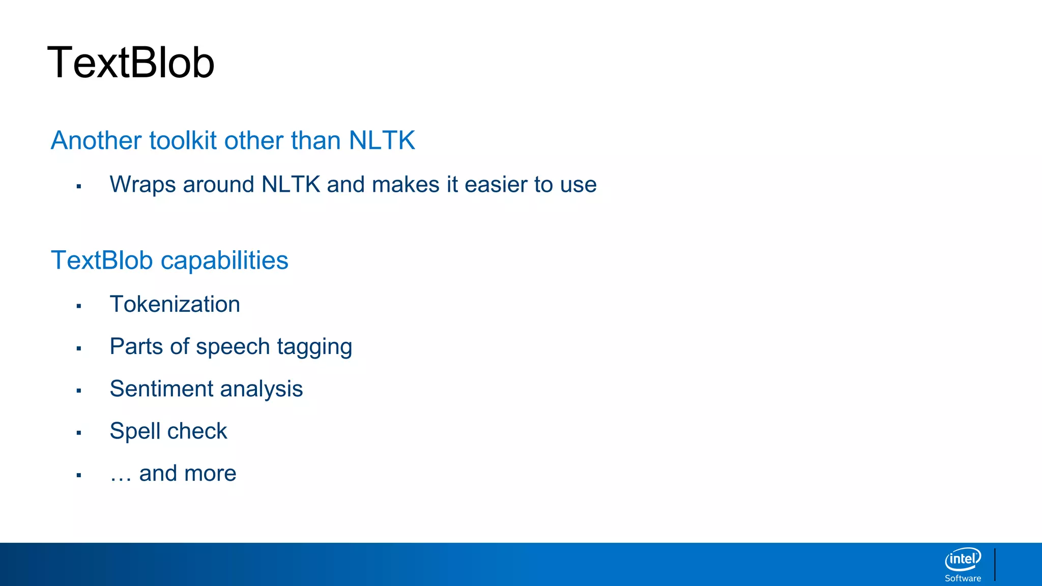
9. TextBlob
Another toolkit other than NLTK
▪ Wraps around NLTK and makes it easier to use
TextBlob capabilities
▪ Tokenization
▪ Parts of speech tagging
▪ Sentiment analysis
▪ Spell check
▪ … and more

10. TextBlob Demo: Tokenization
# Command line: pip install textblob
from textblob import TextBlob
my_text = TextBlob("We're moving from NLTK to TextBlob. How fun!")
my_text.words
Input:
Output:
WordList(['We', "'re", 'moving', 'from', 'NLTK', 'to', 'TextBlob', 'How',
'fun'])

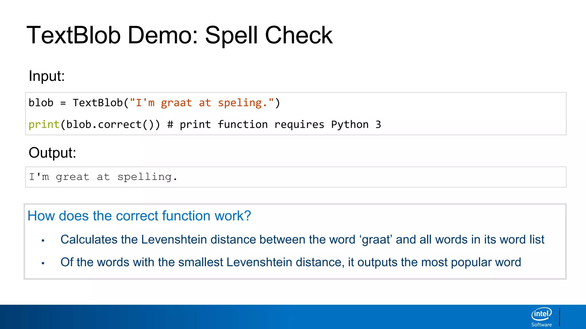
11. TextBlob Demo: Spell Check
blob = TextBlob("I'm graat at speling.")
print(blob.correct()) # print function requires Python 3
Input:
Output:
I'm great at spelling.
How does the correct function work?
▪ Calculates the Levenshtein distance between the word ‘graat’ and all words in its word list
▪ Of the words with the smallest Levenshtein distance, it outputs the most popular word

12. Text Similarity Measures Checkpoint
• Word Similarity
▪ Levenshtein distance
• Document Similarity
▪ Count vectorizer and the document-term matrix
▪ Bag of words
▪ Cosine similarity
▪ Term frequency-inverse document frequency (TF-IDF)

13. Document Similarity
When is document similarity used?
▪ When sifting through a large number of documents and trying to find similar ones
▪ When trying to group, or cluster, together similar documents
To compare documents, the first step is to put them in a similar format so they
can be compared
▪ Tokenization
▪ Count vectorizer and the document-term matrix

14. Text Format for Analysis
There are a few ways that text data can be put into a standard format for analysis
“This is an example”
Split Text Into Words
[‘This’,’is’,’an’,’example’]
One-Hot EncodingTokenization
Numerically Encode Words
This [1,0,0,0]
is [0,1,0,0]
an [0,0,1,0]
example [0,0,0,1]
This slide could make more sense

15. Text Format for Analysis: Count Vectorizer
import pandas as pd
from sklearn.feature_extraction.text import CountVectorizer
corpus = ['This is the first document.',
'This is the second document.',
'And the third one. One is fun.’]
cv = CountVectorizer()
X = cv.fit_transform(corpus)
pd.DataFrame(X.toarray(),columns=cv.get_feature_names())
Input:
Output:
A Corpus is a collection of texts
This is called a
Document-Term Matrix

16. Text Format for Analysis: Key Concepts
The Count Vectorizer helps us create a Document-Term Matrix
• Rows = documents
• Columns = terms
corpus = ['This is the first document.',
'This is the second document.',
'And the third one. One is fun.’]

17. Text Format for Analysis: Key Concepts
Bag of Words Model
• Simplified representation of text,
where each document is recognized
as a bag of its words
• Grammar and word order are
disregarded, but multiplicity is kept

18. Document Similarity Checkpoint
What was our original goal? Finding similar documents.
To compare documents, the first step is to put them in a similar format so they
can be compared
▪ Tokenization
▪ Count vectorizer and the document-term matrix
The big assumption that we’re making here is that each document is just a
Bag of Words

19. Document Similarity: Cosine Similarity
Cosine Similarity is a way to quantify the similarity between documents
• Step 1: Put each document in vector format
• Step 2: Find the cosine of the angle between the documents
“I love you”
“I love NLP”
i love you nlp
Doc 1 1 1 1 0
Doc 2 1 1 0 1
a = [1, 1, 1, 0]
b = [1, 1, 0, 1]
= 0.667
Cosine similarity measures the similarity between two non-zero vectors with the cosine of the angle between them.

20. from numpy import dot
from numpy.linalg import norm
cosine = lambda v1, v2: dot(v1, v2) / (norm(v1) * norm(v2))
cosine([1, 1, 1, 0], [1, 1, 0, 1])
Document Similarity: Cosine Similarity
0.667

21. Document Similarity: Example
Here are five documents. Which ones seem most similar to you?
“The weather is hot under the sun”
“I make my hot chocolate with milk”
“One hot encoding”
“I will have a chai latte with milk”
“There is a hot sale today”
Let’s see which ones are most similar from a mathematical approach.

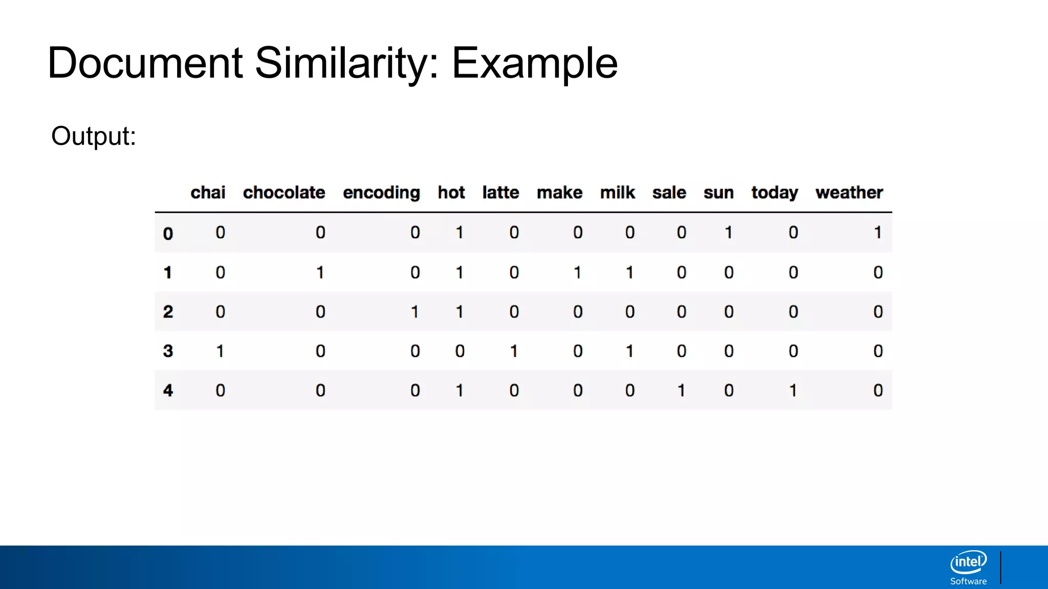
22. Document Similarity: Example
import pandas as pd
from sklearn.feature_extraction.text import CountVectorizer
corpus = ['The weather is hot under the sun',
'I make my hot chocolate with milk',
'One hot encoding',
'I will have a chai latte with milk',
'There is a hot sale today']
# create the document-term matrix with count vectorizer
cv = CountVectorizer(stop_words="english")
X = cv.fit_transform(corpus).toarray()
dt = pd.DataFrame(X, columns=cv.get_feature_names())
dt
Input:

23. Document Similarity: Example
Output:

24. Document Similarity: Example
# calculate the cosine similarity between all combinations of documents
from itertools import combinations
from sklearn.metrics.pairwise import cosine_similarity
# list all of the combinations of 5 take 2 as well as the pairs of phrases
pairs = list(combinations(range(len(corpus)),2))
combos = [(corpus[a_index], corpus[b_index]) for (a_index, b_index) in pairs]
# calculate the cosine similarity for all pairs of phrases and sort by most similar
results = [cosine_similarity([X[a_index]], [X[b_index]]) for (a_index, b_index) in
pairs]
sorted(zip(results, combos), reverse=True)
Input:

25. Document Similarity: Example
[(0.40824829, ('The weather is hot under the sun', 'One hot encoding')),
(0.40824829, ('One hot encoding', 'There is a hot sale today')),
(0.35355339, ('I make my hot chocolate with milk', 'One hot encoding')),
(0.33333333, ('The weather is hot under the sun', 'There is a hot sale today')),
(0.28867513, ('The weather is hot under the sun', 'I make my hot chocolate with milk')),
(0.28867513, ('I make my hot chocolate with milk', 'There is a hot sale today')),
(0.28867513, ('I make my hot chocolate with milk', 'I will have a chai latte with milk')),
(0.0, ('The weather is hot under the sun', 'I will have a chai latte with milk')),
(0.0, ('One hot encoding', 'I will have a chai latte with milk')),
(0.0, ('I will have a chai latte with milk', 'There is a hot sale today'))]
Output:
▪ These two documents are most similar, but it’s
just because the term “hot” is a popular word
▪ “Milk” seems to be a better differentiator, so how
we can mathematically highlight that?

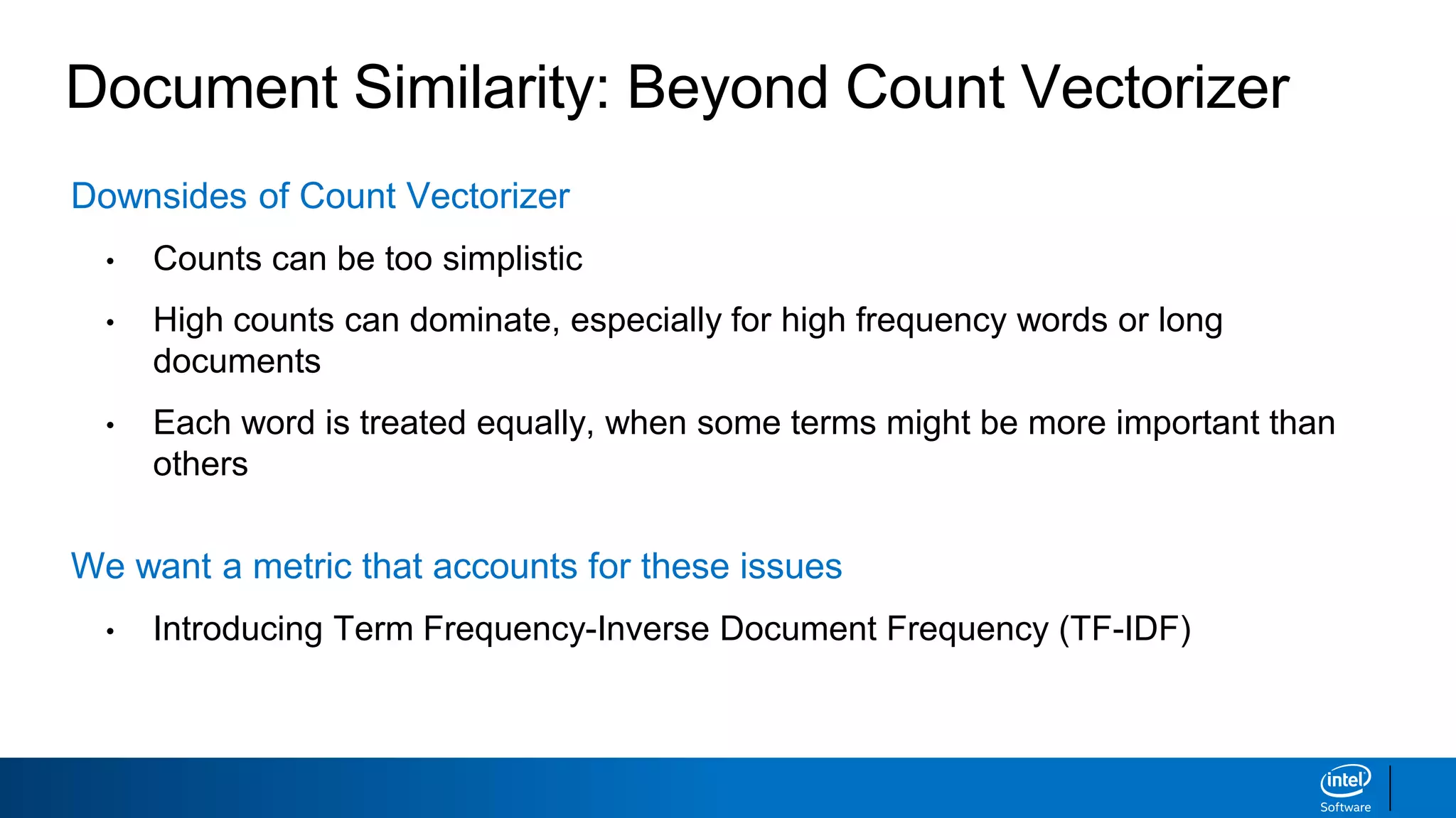
26. Document Similarity: Beyond Count Vectorizer
Downsides of Count Vectorizer
• Counts can be too simplistic
• High counts can dominate, especially for high frequency words or long
documents
• Each word is treated equally, when some terms might be more important than
others
We want a metric that accounts for these issues
• Introducing Term Frequency-Inverse Document Frequency (TF-IDF)

27. Term Frequency-Inverse Document Frequency
TF-IDF = (Term Frequency) * (Inverse Document Frequency)
log( )
+1
+1
Different value
for every
document / term
combination
Term Count in
Document
Total Terms in
Document
Total Documents
Documents Containing
the Term

28. Term Frequency-Inverse Document Frequency
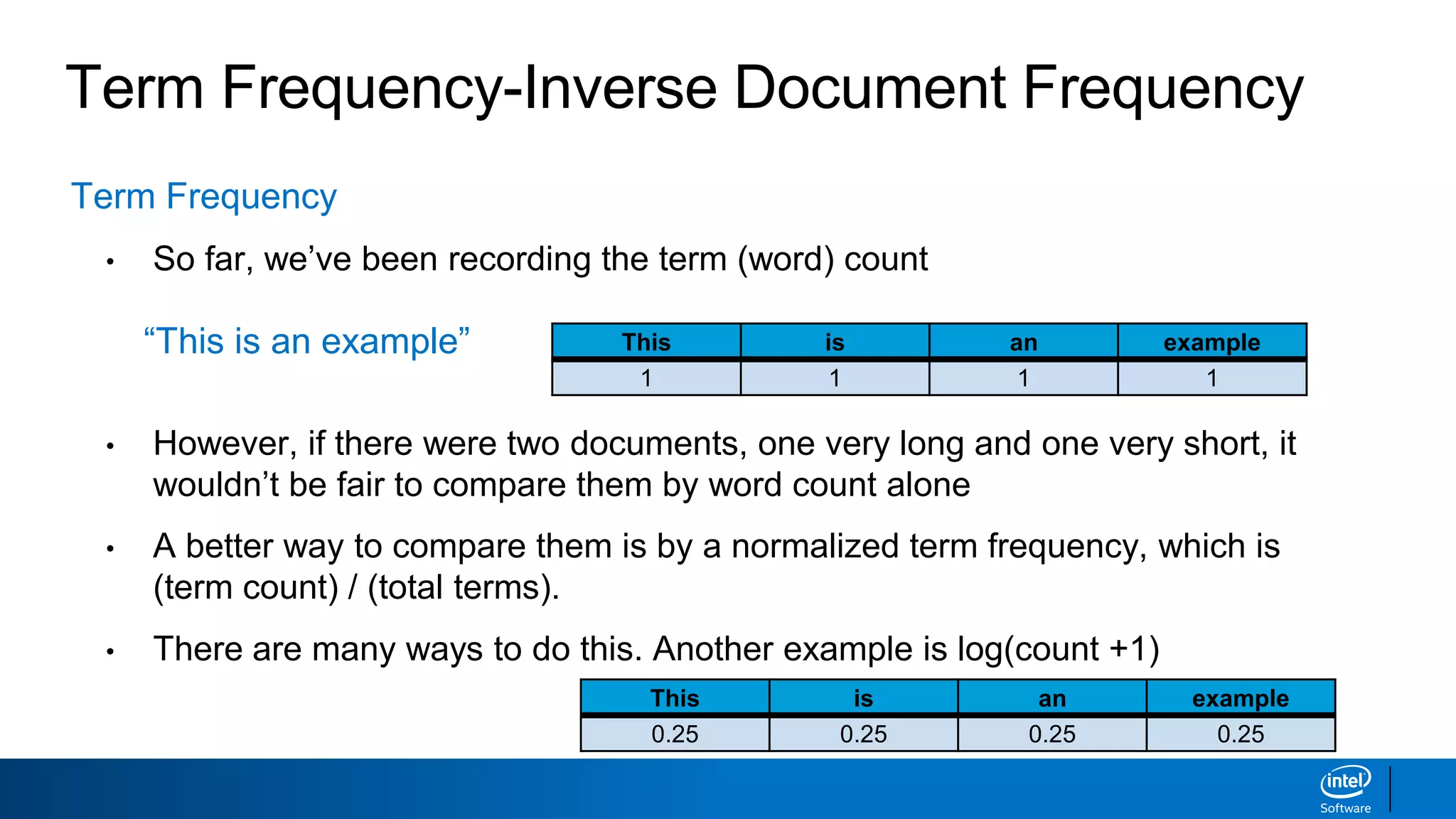
Term Frequency
• So far, we’ve been recording the term (word) count
“This is an example”
• However, if there were two documents, one very long and one very short, it
wouldn’t be fair to compare them by word count alone
• A better way to compare them is by a normalized term frequency, which is
(term count) / (total terms).
• There are many ways to do this. Another example is log(count +1)
This is an example
1 1 1 1
This is an example
0.25 0.25 0.25 0.25

29. Term Frequency-Inverse Document Frequency
Inverse Document Frequency
• Besides term frequency, another thing to consider is how common a word is
among all the documents
• Rare words should get additional weight
Total Documents
Documents Containing
the Term +1
+1 Want to make
sure that the
denominator is
never 0
log( )
The log
dampens the
effect of IDF

30. Term Frequency-Inverse Document Frequency
TF-IDF = (Term Frequency) * (Inverse Document Frequency)
log( )
+1
+1
Different value
for every
document / term
combination
Term Count in
Document
Total Terms in
Document
Total Documents
Documents Containing
the Term

31. Term Frequency-Inverse Document Frequency
TF-IDF Intuition:
• TF-IDF assigns more weight to rare words and less weight to commonly
occurring words.
• Tells us how frequent a word is in a document relative to its frequency in
the entire corpus.
• Tells us that two documents are similar when they have more rare words
in common.

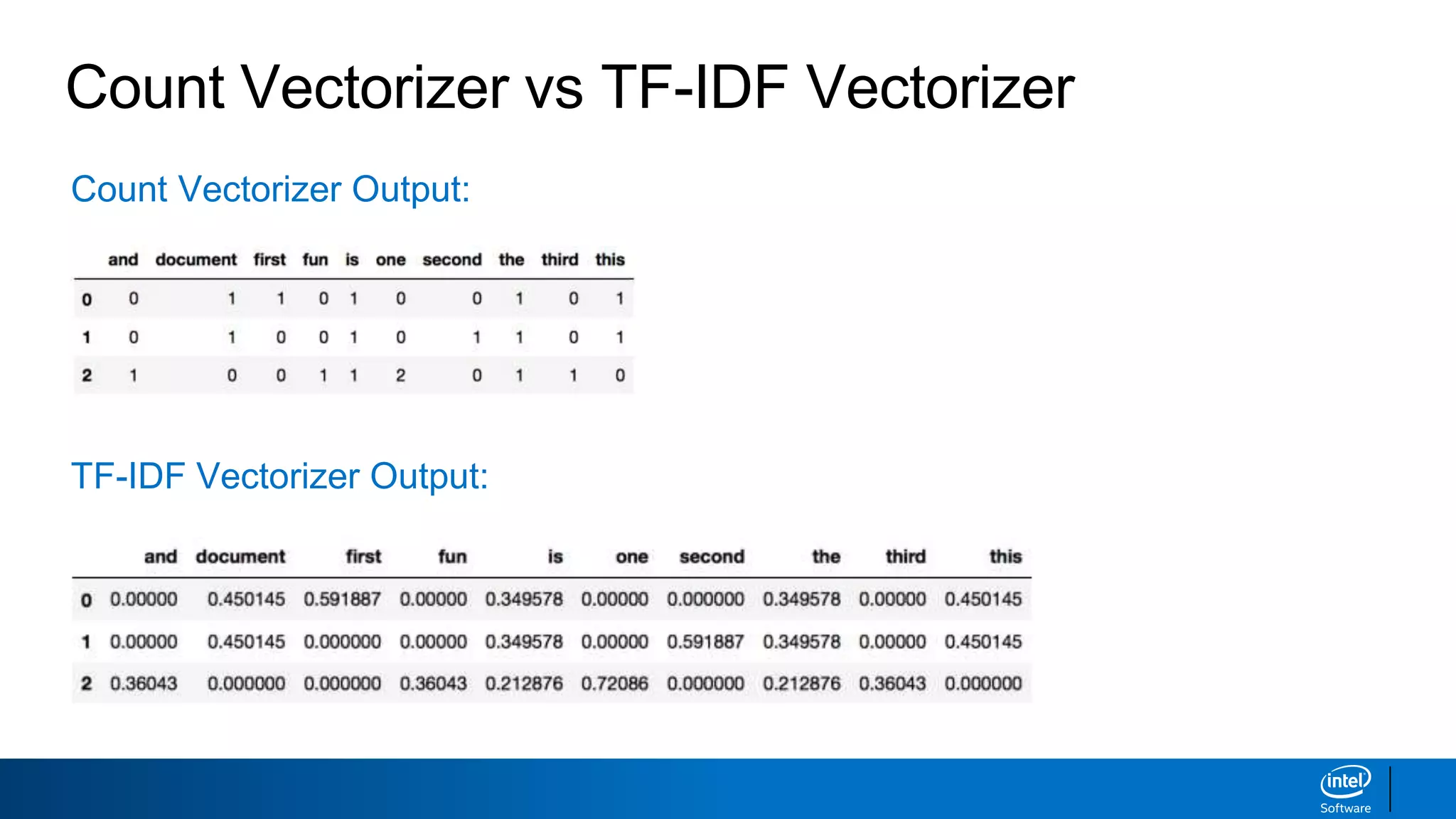
32. Count Vectorizer vs TF-IDF Vectorizer
import pandas as pd
corpus = ['This is the first document.',
'This is the second document.',
'And the third one. One is fun.’]
# original Count Vectorizer
from sklearn.feature_extraction.text import CountVectorizer
cv = CountVectorizer()
X = cv.fit_transform(corpus).toarray()
pd.DataFrame(X, columns=cv.get_feature_names())
# new TF-IDF Vectorizer
from sklearn.feature_extraction.text import TfidfVectorizer
cv_tfidf = TfidfVectorizer()
X_tfidf = cv_tfidf.fit_transform(corpus).toarray()
pd.DataFrame(X_tfidf, columns=cv_tfidf.get_feature_names())

33. Count Vectorizer vs TF-IDF Vectorizer
Count Vectorizer Output:
TF-IDF Vectorizer Output:

34. Document Similarity: Example
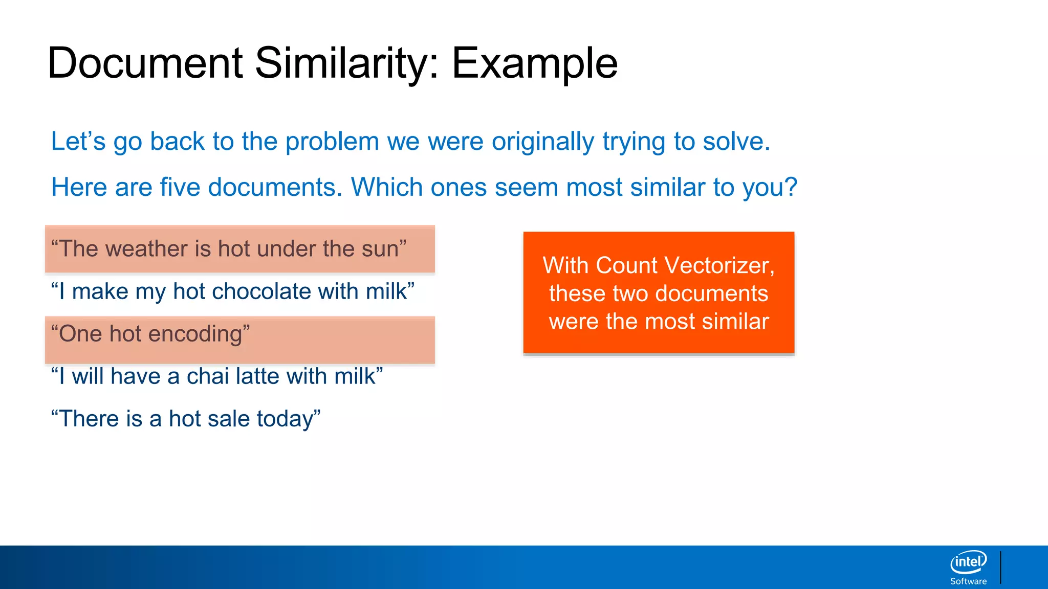
Let’s go back to the problem we were originally trying to solve.
Here are five documents. Which ones seem most similar to you?
“The weather is hot under the sun”
“I make my hot chocolate with milk”
“One hot encoding”
“I will have a chai latte with milk”
“There is a hot sale today”
With Count Vectorizer,
these two documents
were the most similar

35. Document Similarity: Example with TF-IDF
from sklearn.feature_extraction.text import TfidfVectorizer
# create the document-term matrix with TF-IDF vectorizer
cv_tfidf = TfidfVectorizer(stop_words="english")
X_tfidf = cv_tfidf.fit_transform(corpus).toarray()
dt_tfidf = pd.DataFrame(X_tfidf,columns=cv_tfidf.get_feature_names())
dt_tfidf
Input:
Output:

36. Document Similarity: Example with TF-IDF
# calculate the cosine similarity for all pairs of phrases and sort by most similar
results_tfidf = [cosine_similarity(X_tfidf[a_index], X_tfidf[b_index])
for (a_index, b_index) in pairs]
sorted(zip(results_tfidf, combos), reverse=True)
[(0.23204485, (‘I make my hot chocolate with milk', 'I will have a chai latte with
milk')),
(0.18165505, ('The weather is hot under the sun', 'One hot encoding')),
(0.18165505, ('One hot encoding', 'There is a hot sale today')),
(0.16050660, ('I make my hot chocolate with milk', 'One hot encoding')),
(0.13696380, ('The weather is hot under the sun', 'There is a hot sale today')),
(0.12101835, ('The weather is hot under the sun', 'I make my hot chocolate with milk')),
(0.12101835, ('I make my hot chocolate with milk', 'There is a hot sale today')),
(0.0, (‘The weather is hot under the sun', 'I will have a chai latte with milk')),
(0.0, ('One hot encoding', 'I will have a chai latte with milk')),
(0.0, ('I will have a chai latte with milk', 'There is a hot sale today'))]
By weighting “milk” (rare) > “hot” (popular), we get a smarter similarity score

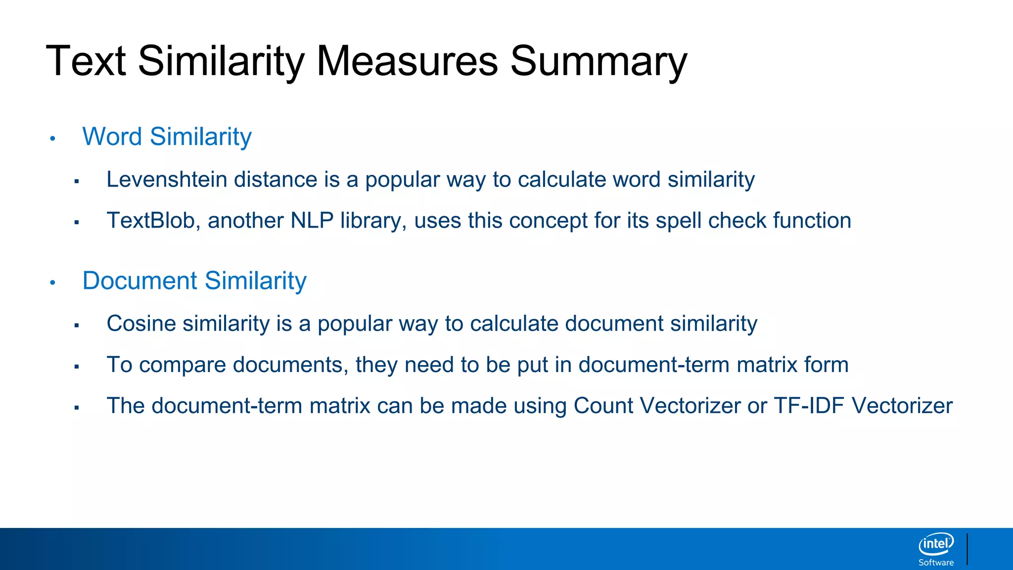
37. Text Similarity Measures Summary
• Word Similarity
▪ Levenshtein distance is a popular way to calculate word similarity
▪ TextBlob, another NLP library, uses this concept for its spell check function
• Document Similarity
▪ Cosine similarity is a popular way to calculate document similarity
▪ To compare documents, they need to be put in document-term matrix form
▪ The document-term matrix can be made using Count Vectorizer or TF-IDF Vectorizer